Long-range dependence in the runoff time series of the most important Patagonian river draining to the Pacific Ocean

ABSTRACT

The Baker River is the largest free-flowing river in Chilean Patagonia. Long-range dependence (LRD), a recognised hydrological property of river runoff worldwide, was detected for the Baker River runoff time series. Analyses were conducted on a monthly scale between 1961 and 2015 using the fractal and multifractal detrended fluctuation analysis methodology. A long-range-dependent Hurst coefficient (H) equal to 0.94 was obtained. A scaling range, which is the signature of LRD, was detected for the Baker River runoff time series between 1 and 5.25 years. Baker River runoff showed a strong correlation (r = 0.96) with the Antarctic Oscillation (AAO) Index during the 2007–2015 period. The high storage capacity of Lake General Carrera, the size of the Baker River basin area and the dynamics of AAO are proposed as main factors that contribute to the emergence of LRD in the Baker River runoff time series.

KEYWORDS:

• Long-range dependence
• multifractality
• Hurst coefficient
• Baker River
• Patagonia
• Antarctic Oscillation Index
• Chile

Introduction

Over the last decade, much research effort was focused on the analysis and interpretation of long-range dependence (LRD), also called long-term or long-range persistence (LTP), in river runoff time series within the framework of fractal theory (Kantelhardt et al. 2006; Koscielny-Bunde et al. 2006; Witt and Malamud 2013). Fractality is the signature of scaling, also known as the power law process, which is a process characterised by LRD between observations (Samorodnitsky and Taqqu 1994; Seuront 2010).

Long-range-dependent time series exhibit an autocovariance function that decays slowly over time, which means that observations separated by long time intervals exhibit non-zero covariance (Beran et al. 2013). Traditionally, ever since the work of Mandelbrot and van Ness (1968), the Hurst coefficient (H) has been used as a measure of LRD or long-range memory. However, in many cases river runoff time series exhibit a richer and more complex dynamics called multifractality. Multifractality implies intermittent behaviour of time series in addition to LRD (Seuront 2010) and can be considered as a ‘fingerprint’ of river runoff that serves to understand its temporal dynamics better (Kantelhardt et al. 2003). Few attempts have been made to quantify the LRD of South American rivers (e.g. Prass et al. 2012), for which databases are scarce and highly fragmented. Multifractal dynamics in river runoff time series have also been poorly studied in South American rivers, and to the best of our knowledge, only two studies (Hansen and Seoane 2013; Rego et al. 2013) have been conducted to date. Both studies were focused on rivers draining to the Atlantic Ocean. Consequently, it is highly relevant to study the long-range temporal dynamics and multifractality of rivers draining into the Pacific such as the Baker River, which is free flowing and the largest river in Chilean Patagonia. Moreover, studying the Baker River has become even more important given plans to dam this river (e.g. HidroAysén 2008), and the evidence that man-made constructions severely affect the multifractal dynamics of rivers (Rego et al. 2013).

Patagonia is a continental landmass that emerges at mid-latitudes in the Southern Hemisphere, encompassing Pacific and Atlantic lowlands and coasts, valleys, archipelagos, tablelands and high plains (Coronato et al. 2008). It is a nearly pristine environment that extends from 37°S to Cape Horn, made up of unique aquatic and terrestrial ecosystems (Mazzoni et al. 2010); it contains the third most important reserve of freshwater in the world (Vince 2010) and includes a high diversity of lakes, rivers and fjords (Dussaillant et al. 2012). The fjord region provides essential ecosystem services, which are often ignored in the assessment of development projects; it is now considered a highly vulnerable region (Iriarte et al. 2010). In particular, the Baker fjord was classified as having a good to high ecological status, strongly influenced by high levels of freshwater input from glacial discharges (Quiroga et al. 2013).

The Baker River basin extends over approximately 26,000 km² and is located in the northern area of Chilean and Argentinean Patagonia, between 45°50' and 47°55' S (Lobos et al. 1987) (Figure 1). It includes the second largest lake in South America, General Carrera Lake (surface area 978.12 km²; Atlas Región de Aysén 2005) and also includes the Laguna San Rafael biosphere reserve located within the Northern Patagonian Icefield (Moreira-Muñoz et al. 2014). The Chilean portion of the basin (over 17,000 km²) is located in the Aysén Region. This region has been under considerable pressure due to the HidroAysén project, which involves the construction of five hydroelectric dams on the Baker and Pascua rivers. If this highly controversial project goes ahead, the dams will inundate a total of 5910 ha (HidroAysén 2008). For a single dam on the Baker River (Baker 1, flooding 710 ha), the associated environmental costs for landscape loss alone (omitting biodiversity and tourism losses) will total US$720 million (Ponce et al. 2011). Additional pressure on General Carrera Lake is pending due to the recently launched international public tender by the Argentinian Government for the construction of the megaproject ‘Rio Deseado Multipurpose Aqueduct’ that would withdraw water from this binational lake, called Buenos Aires Lake in Argentina, and transport it to the northern zone of the Argentinian Santa Cruz province (SOP 2015). Furthermore, the salmon aquaculture industry is a continuously growing sector of the Chilean economy and exerts additional stress on this ecosystem, which is one of the most pristine ecosystems in the world (Mittermeier et al. 2003; Bastianon et al. 2012).

Figure 1. Baker River basin including the General Carrera and Bertrand lakes. The gauging station at Lake Bertrand is marked with a triangle (47°03′S; 72°48′W). Baker River and its largest tributaries, the Nef and Colonia rivers, are shown at the bottom of the map above the small village called Caleta Tortel. The Argentinian portion of General Carrera Lake is not shown on the map.

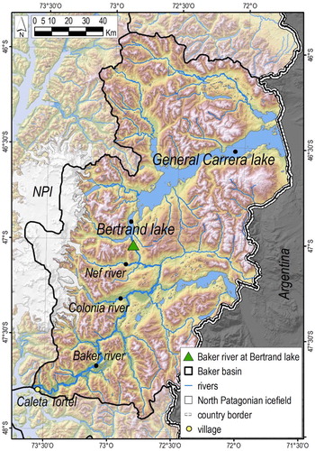
Rivers in Chilean Patagonia flow towards the coastal zone into the fjords, which are connected to the Pacific Ocean. Their flow is usually regulated by several lakes, forming a continuous lake–river–fjord corridor (Niemeyer and Cereceda 1984). The Baker River is the largest river in Chile in terms of water flow (1500 m³/s), the longest in the region (175 km length) (Atlas Región de Aysén 2005), and one of the three largest free-flowing rivers in Patagonia (Tagliaferro et al. 2013). It has an annual flow peak in late summer/early autumn (January–March) and a minimum during early spring (September) (Zambrano et al. 2009). The Baker River flows out of Bertrand Lake, which receives the overflow of the General Carrera/Buenos Aires Lake and empties into the Baker Channel close to the village of Caleta Tortel, which has approximately 500 inhabitants (Atlas Región de Aysén 2005; Figure 1). Its greatest tributaries, the Nef and Colonia rivers, come from the Northern Patagonia Ice Field (López et al. 2008) (Figure 1).

The Baker River flows southwest and plays a major role in structuring the spatial dynamics of zooplankton (Meerhoff et al. 2013), and also in the distribution, growth and feeding of larval stages of fish that inhabit Patagonian fjord ecosystems (Landaeta et al. 2012). Indeed, it has been detected that changes in Baker River runoff levels above specific thresholds can directly affect the physical structure of the water column, enhancing its biological productivity (Ross et al. 2014).

River flows fluctuate over many time scales as the result of the interaction between stochastic and deterministic forging (Huang et al. 2009), in which rainfall, topography and geography play major roles (Schumm 2005). In this study, we were interested in the stochastic properties of the Baker River runoff time series, and for that reason the annual cycle of runoff was removed before the quantification of LRD. Scaling dynamics in river runoff time series is not new (Tessier et al. 1996), but fractal research has been mainly focused on detecting and quantifying LRD in Northern Hemisphere rivers (Kantelhardt et al. 2006; Rybski et al. 2011; Markovic and Koch 2013; Szolgayova et al. 2014) and little information on LRD is available for Southern Hemisphere rivers. The geographical location of the Baker River gives us the opportunity to quantify LRD (if detected) in a Southern Hemisphere river and also to test specific hypotheses about its possible origin. We expect a high level of LRD in the Baker River runoff time series, because it drains freshwater from two large reservoirs: the Northern Patagonia Icefield which includes 28 glaciers with an ice surface area of about 4200 km² (Aniya 1988) and General Carrera Lake (1850 km², Mazzoni et al. 2010) (Figure 1). The continuous freshwater contribution of both reservoirs through time makes it likely that monthly runoff values are strongly correlated well beyond the seasonal time scale.

We know that the Antarctic Oscillation (AAO) Index, also called the Southern Annular Mode (SAM), is the dominant mode of climatic variability at higher latitudes in the Southern Hemisphere (Thompson and Wallace 2000, Garreaud et al. 2009), and appears to be the main climatic forcing of the Baker River (Lara et al. 2015). It is important to note that the El Niño Southern Oscillation (ENSO) has less influence on the climatic variability of Patagonia at this latitude (between ca. 45° and 47°S) (Aravena and Luckman 2009). Consequently, the AAO Index could affect the temporal dynamics of Baker River runoff at inter-annual time scales, and also the extension of its scaling range if LRD is detected.

Thus our objectives were: (i) to detect and quantify LRD and multifractality in monthly runoff observations of the Baker River time series in an effort to characterise baseline conditions of flows prior to any major human intervention, (ii) to test if the scaling range of Baker River runoff may be associated with its main climatic forcing, i.e. the AAO Index, or with the Southern Oscillation Index (SOI, Lara et al. 2015).

Materials and methods

Baker River runoff time series

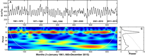
The average monthly runoff of Baker River (Q) for 1961–2015 (55 years) (Figure 2A) was obtained from official reports published by the Chilean Service of Environmental and Impact Assessment (SEA 2016) and by the Chilean General Water Administration (http://www.dga.cl) at the Lake Bertrand gauging station (47°03′S, 72°48′W; Figure 1). A few isolated missing data observations totalling 5 months were estimated by linear interpolation, which represents only 0.75% of the runoff time series. Such a minimal fraction of missing observations prior to the estimation of fractal parameters did not introduce any spurious correlations (Wilson et al. 2003; Montes et al. 2012).

Figure 2. A, Baker River monthly runoff time series (Q, m³/s) from 1961 to 2015. Mean monthly runoff values were obtained from the Lake Bertrand sampling station (Figure 1). Separations between decades are marked with vertical lines. B, Wavelet local power spectrum of runoff time series for the Baker River during the same time period. The red band associated with a periodicity of 12 months corresponds to the annual cycle. White lines indicate the cone of influence that delimits the region not influenced by edge effects. For A and B, the first and last observations correspond to January 1961 and December 2015, respectively. C, Wavelet global power spectrum. The grey line represents the α = 5% significance level. The annual cycle is clearly significant.

AAO Index time series

Monthly values of the AAO Index (Mo 2000; Thompson and Wallace 2000), also called SAM, were obtained from 1979 to 2015 (n = 444) from the National Oceanic and Atmospheric Administration (NOAA, USA) Climate Prediction Center available at http://www.cpc.ncep.noaa.gov/products/precip/CWlink/daily_ao_index/aao/aao_index.html. This index reflects the difference in the mean zonal pressure at sea level between mid and high latitudes (Villalba et al. 2012).

SOI time series

The SOI measures the normalised pressure difference between Tahiti and Darwin. This index was obtained at a monthly scale for the period 1961–2015 (n = 660) from the Climatic Research Unit of the University of East Anglia, UK (https://crudata.uea.ac.uk/cru/data/soi/soi.dat), which was calculated based on the method proposed by Ropelewski and Jones (1987).

Removal of periodicities

Periodic or seasonal components of the runoff time series can distort the estimation of fractal parameters (Montanari et al. 1999; Rybski et al. 2011), and indeed they can mask the fractal dynamics on time scales longer than seasonal (Agarwal et al. 2012). This deterministic component clearly appears as a marked seasonal cycle with high flows during the spring–summer period, driven by snowmelt and ice ablation (Dussaillant et al. 2012). The marked annual cycle of the Baker River runoff time series (Figure 2B,C) was removed by calculating and subtracting for every month the long-term average calculated across years (e.g. January 1961, January 1962, … , January 2015) (Rybski et al. 2011). We are aware that the selection of a specific filtering procedure can severely affect the results (Markovic and Koch 2005). For this reason, the effect of applying a different filtering method to remove the annual cycle from runoff time series based on the continuous wavelet transform (CWT) (Torrence and Compo 1998) was also tested (Appendix 1). After removing the annual cycle, the detrended Baker River runoff time series was used to estimate LRD and multifractal dynamics.

Fractal and multifractal analysis

For the detection and quantification of fractal and multifractal dynamics of Baker River runoff, detrended fluctuation analysis (DFA, Kantelhardt et al. 2001) and multifractal detrended fluctuation analysis (MF-DFA, Rybski et al. 2011) were used, respectively. In addition, the Kettani and Gubner estimator (2006, Appendix 2) was used to compare the consistency between the Hurst coefficient estimated with DFA (H_DFA) and the Hurst coefficient estimated with the KG estimator (H_KG).

Fractal and multifractal detrended fluctuation analysis

DFA has been proved to be useful for the estimation of LRD in non-stationary time series (Kantelhardt et al. 2001); this method was then generalised to higher statistical moments to allow the detection of the multifractal dynamics of runoff time series using the so-called MF-DFA (Kantelhardt et al. 2002; 2006; Koscielny-Bunde et al. 2006; Rybski et al. 2011). For the estimation of a reliable LRD parameter, at least 400 data points are needed (Markovic and Koch 2013; Ludescher et al. 2015); the Baker River runoff time series largely exceeded this threshold (n = 660).

In the initial stage of the DFA methodology, the cumulative sum Y(i), also known as the profile function, was constructed according to:(1) where X(k) represents the runoff time series of length n = 660. The new time series Y(i) obtained using Equation (1) was divided into n/s non-overlapping segments of equal length s. The procedure was then repeated starting from the opposite end of the runoff time series in order to obtain 2n_s segments. For each of the 2n_s segments, a polynomial function of order m, representing the local trend in that segment, was fitted. Here only m = 2 was used, which means that quadratic trends were removed from the profile function. Then, the variance σ was estimated for each segment v after subtracting the local trends. In other words, the fluctuation of the time series was determined as the variance of the estimated local trend. In the final stage, the variances of all segments were averaged and the square root was taken to obtain the mean fluctuation function F(s) as:(2)

Averages of F(s) were calculated over several segments of different size s to analyse the relationship between the mean fluctuation function and segment size. A power law relationship between F(s) and segment size s is the signature of scaling and LRD, which was estimated according to:(3) The scaling exponent or LRD parameter h(2) was estimated by plotting the average root mean square fluctuation function F(s) calculated using Equation (3) versus the segment size s on a double logarithmic scale (Kantelhardt et al. 2001). The slope h(2) of the line obtained from the least squares estimation in Equation (3) represents the strength of LRD, and can be used to estimate the Hurst coefficient (H), a well-known index of LRD (Samorodnitsky and Taqqu 1994).

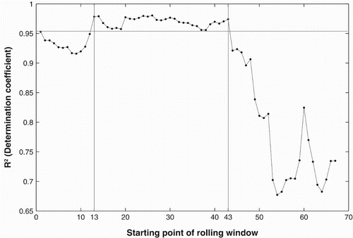
Scaling range was estimated according to the R²-SSR methodology (Seuront 2010), which means that selected scaling range maximised the coefficient of determination (R²) and minimised the total sum of squared residuals (SSR). R² and SSR values were calculated within a rolling window of 13 months (Maraun et al. 2004) to analyse the behaviour of the mean fluctuation function F(s) across time lags. R² values should reach maximum values (close to 1) within the range where scaling is claimed (Seuront 2010). The maximum segment size for the detection of the scaling range was set to one-fourth (n/4) of the time series length. Above n/4, the fluctuations of F(s) increase due to the reduced number of segments used in its calculation, and hence the estimation of F(s) becomes unreliable (Kantelhardt 2009).

For the multifractal time series analysis, a generalisation to higher statistical moments is necessary. In this framework, the variance σ (v, s) from Equation (2) is replaced by the q/2th power, and the square root is replaced by the 1/qth power (Kantelhardt et al. 2006) as:(4) In a similar way to the definition in Equation (3), the generalised fluctuation exponent h(q) can be obtained from:(5)

For the special case for the statistical moment q = 2, this method is equivalent to the standard DFA (Kantelhardt et al. 2006). For stationary time series, h(2) corresponds to the Hurst coefficient and hence h(q) is designated as the generalised Hurst exponent (Kantelhardt et al. 2002). For fractal (monofractal) time series, the h(q) exponent is independent of q. For this type of time series, the scaling behaviour of the variances is equal for all time scales and q values. For multifractal time series, a single scaling exponent such as h(2) is not sufficient to characterise their dynamics completely, since many subsets of the time series have different scaling behaviour.

Monte Carlo testing

The estimation of LRD constrained by time series length has been a controversial issue (Percival et al. 2001; Khaliq et al. 2008). For this reason, we followed Khaliq et al. (2008) and used Monte Carlo simulation to estimate confidence intervals of Hurst coefficients for multiple uncorrelated time series. To verify if our results are significantly different from H = 0.5, R = 1000 white noise time series of equal size to the Baker River runoff (n = 660) were simulated. Hurst coefficients for simulated time series were estimated with the DFA methodology, 95% confidence intervals were calculated, and results were compared with the Hurst coefficient previously obtained for Baker River. Using the same methodology, simulated time series were used to verify if Baker River runoff is better described by a fractal than by a multifractal process.

Results

A clear scaling range was detected for the Baker River runoff time series, which extends between 12 and 63 months (1–5.25 years) (Figure 3). Maximum R² values associated with this scaling range are shown in Figure 4. The slope h(2) of this scaling range was estimated as 0.94. Consequently, the Hurst coefficient (H_DFA), was calculated as H_DFA = h(2) = 0.94 (Kantelhardt et al. 2006). On the other hand, the Hurst coefficient obtained using the KG estimator (H_KG, Appendix 2, Equation (2.1)) was equal to H_KG= 0.93. When the annual cycle of Baker River runoff was removed using CWT (Appendix 1) instead of long-term averages, the Hurst coefficient obtained with DFA was H_DFA = 0.98 and with the KG estimator was H_KG = 0.92. According to these results, the detrended runoff time series of the Baker River can be considered as highly persistent (H tends to 1) independent of the method used for removing the annual cycle. Persistence means that if runoff levels increase (or decrease) for a period of time, they are expected to continue increasing (decreasing) for a similar period of time.

Figure 3. Root mean square fluctuation function F(s) on a logarithmic scale for the Baker River runoff time series between 1961 and 2015. Scaling range (between vertical lines) extends between 12 and 63 months (ca. 1 and 5.3 years), for which h(2) equals 0.94.

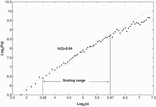
Figure 4. Determination coefficient (R²) calculated within rolling windows of length equal to 13. The first and second data points correspond to R² values calculated between 1 and 13 months and between 2 and 14 months, respectively. The starting point of maximum and stable R² values (above 0.95) was obtained for the rolling window marked with a vertical line at point 13, which corresponds to 12 months (1 year). The ending point of maximum R² was obtained for the rolling window marked with a vertical line at point 43, which extends up to 63 months (5.25 years). According to these results, the scaling range extends between 1 and 5.25 years.

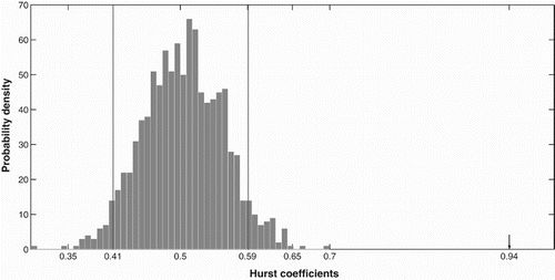
The effect of time series length on LRD parameters is shown in Figure 5. As can be observed in this figure, lower and upper confidence intervals of Hurst coefficients for white noise time series (H_L, H_U) were calculated as H_L = 0.41 and H_U = 0.59, respectively. As the Hurst coefficient estimated for Baker River (H_DFA = 0.94, Figure 5) is clearly above the upper confidence limit estimated for a white noise process (H_U = 0.59) (Figure 5), it can be concluded that the runoff time series is significantly different from the uncorrelated time series. On the contrary, the Baker River runoff showed strong persistence or LRD.

Figure 5. Hurst coefficients obtained for 1000 Monte Carlo simulated white noise time series and calculated with the DFA methodology. Lower and upper 95% confidence intervals are marked with vertical lines. The Hurst coefficient for Baker River runoff is marked with an arrow.

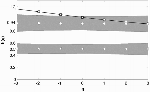
In the same way, Monte Carlo simulated time series were used to discriminate if Baker River runoff is better described by a fractal than by a multifractal process. R = 1000 white noise time series (H = 0.5) and R = 1000 fractal time series with the same Hurst coefficient (H = 0.94) and time series length (n = 660) of the Baker River runoff were simulated. Simulations were conducted in R software (R Development Core Team 2005, version 3.0.2) according to the method described in Davies and Harte (1987) using the R package ‘fracdiff’ (Fraley et al. 2006). The behaviour of generalised Hurst coefficients (h(q)s) for simulated time series between q = −3 and q = + 3 was compared to the behaviour of generalised Hurst coefficients estimated for the Baker River runoff. Figure 6 shows that the behaviour of a fractal time series with H = 0.94 and n = 660 is not significantly different from Baker River generalised Hurst coefficients for all statistical moments. Indeed, h(q)s for Baker River fall within the 95% confidence limits for simulated fractal time series between q = −0.5 and q = 3 (Figure 6). As q increases, h(q)s for the Baker River time series approximate the mean value of h(q) estimated for simulated fractal time series, and when it reaches q = 3 the h(q)s are indistinguishable (Figure 6). A similar behaviour of h(q)s was detected by Ludescher et al. (2011) for fractal time series corrupted with short-range correlations, which result in spurious multifractality. In these cases, only large q values can be considered for the estimation of h(q)s (Ludescher et al. 2011). When q = 2, h = 0.94 for the Baker River runoff time series, and the mean value of h for simulated fractal time series is only slightly lower (h = 0.92, Figure 6). This means that Baker River runoff dynamics is better described by a fractal than by a multifractal model and that short-range correlations are present in the Baker River runoff time series.

Figure 6. Generalised Hurst coefficients (h(q)s) estimated with the MF-DFA method obtained for 1000 Monte Carlo simulated white noise time series (triangles) and fractal Gaussian noise series with H = 0.94 (circles). h(q)s for the Baker River runoff time series are represented by squares connected by a continuous line. All time series have equal length (n = 660). Lower and upper 95% confidence intervals for white noise and fractional Gaussian noise time series are delimited by grey areas.

Relationship between the AAO Index and the Baker River runoff time series

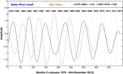
As the scaling range of Baker River runoff extends up to 5.25 years (63 months), reconstructions of the Baker River and the AAO Index time series were conducted using CWT (Torrence and Compo 1998, Equation (1.1)) (Appendix1), focusing on monthly scales between j₁= 62 and j₂= 64. Reconstructed time series are shown in Figure 7. Two different general patterns of variability are visible in this figure: (i) Baker River runoff and AAO Index time series appear to be out of phase between 1979 and 2006 with a moderate negative correlation between the two time series (r = −0.43) and (ii) a strong correlation between Baker River runoff and the AAO Index from 2007 onwards (r = 0.96). This coupled temporal dynamics detected at 5.25 years scale of variability suggests that the AAO Index could play a major role in structuring the LRD detected in the Baker River runoff time series.

Figure 7. Reconstructed Baker River runoff and Antarctic Oscillation (AAO) Index time series using CWT. Scales between j₁= 62 and j₂= 64 months were used to reconstruct both series. Correlation coefficient (r) between Baker River runoff and AAO for (i) 1979–2006 period equals −0.43, and for (ii) 2007–2015 period equals 0.96.

Relationship between the SOI and the Baker River runoff time series

The same time scales (j₁= 62 and j₂= 64 months) were used for the reconstruction of the SOI time series. The correlation between the SOI and the Baker River runoff reconstructed time series is not marked (not shown). The correlation between the time series from 1979 to 2006 is low (r = −0.29), but it increased to r = −0.58 between 2007 and 2015.

Discussion

Long-range dependence

The marked Hurst coefficient detected for the Baker River runoff time series, and its scaling range which extends beyond several years (5.25 years), are similar to those found for European and North American rivers (Pandey et al. 1998; Koscielny-Bunde et al. 2006; Rybski et al. 2011). We are confident that the Hurst coefficient obtained for Baker River runoff is indicative of a highly persistent or long-memory process, according to its value (H = 0.94) and to the runoff time series length (n = 660 observations). For long-range-dependent time series shorter than the Baker River runoff time series (n = 500), the standard errors of the slope h(2) obtained using DFA are equal to 0.10 (Bashan et al. 2008; Kantelhardt 2009). This means that in the worst-case scenario, the Hurst coefficient (H) of Baker River runoff could decrease to 0.84, which is still indicative of a persistent process and clearly above the value obtained for an uncorrelated white noise time series, for which H = 0.5.

The LRD detected for the Baker River runoff time series could be explained in general terms by the flow regime of the Baker River, characterised by very stable discharges due to the buffering capacity of General Carrera Lake (Dussaillant et al. 2012). Similar results were found when analysing the effect of dams and lakes on the LTP of Yangtze River flow (China). For this river, the estimated h(2) was 0.97 (Zhang et al. 2012), but calculations were conducted for time scales smaller than those used for Baker River. We would like to point out that LTP has been detected for the Argentinian Patagonian Neuquén River, with Hurst coefficients varying between 0.81 and 0.89 for a similar time period (1961–2011) (Hansen and Seoane 2013). In addition, for lakes located in Argentinian Patagonia water level variability has a persistent temporal dynamics characterised by Hurst coefficients varying between 0.69 and 0.91 depending on spatial locations (Pasquini et al. 2008). Long-term memory in runoff time series can also be interpreted as the result of aggregation of short-memory contributions coming from reservoirs that form a network of tributaries (Mudelsee 2007). This hypothesis is less plausible for the case of Baker River runoff because the Bertrand Lake gauging station is located above the contribution of major tributaries (e.g. Nef and Colonia rivers, Figure 1) takes place.

There is evidence that flow regimes dominated by snow melting tend to smooth out fluctuations between years, which results in lower Hurst coefficients than those obtained for runoff time series from rivers located in catchments where snowmelt is less important (Szolgayova et al. 2014). Rainfall and snowmelt in the Baker River basin contributed almost equally (13.5% vs. 8.3%, respectively) to the formation of flows in this ecosystem (Krogh et al. 2015). For this reason, the hypothesis which sustains that snowmelt-melting flow regimes are associated with low Hurst coefficients has less support for the Baker River. However, we believe that snowmelt can affect the temporal dynamics of Baker River flow at short time scales, considering that its effect can contribute to the flow up to 6 months per year (Krogh et al. 2015). The extension of the scaling range found for Baker River runoff (5.25 years) may be related to (i) the inter-annual component of 5.1 years of the rainfall temporal dynamics which explains 20% of the variance (Aravena and Luckman 2009) and/or (ii) the inter-annual AAO Index oscillation, which has a low-frequency component between 5.1 and 6.0 years that explains 14.7% of the variance (Valdés-Pineda et al. 2017).

It is interesting to examine the link between the river basin area and the degree of LRD for different rivers worldwide. It appears that the increment of each river basin is followed by an increase in LRD (Mudelsee 2007; 2010; Szolgayova et al. 2014). For the Baker River basin area (area = 26,000 km²), a Hurst coefficient close to 1 is expected according to the dependency found by Hirpa et al. (2010) in an analysis of 14 gauging stations in the southeastern United States using the same methodology (DFA) utilised here for the estimation of LRD. The Hurst coefficient of ca. 0.98 was estimated for a river basin of similar size (19,600 km², Hirpa et al. 2010) to the Baker River basin which closely matches our results (H = 0.94). Moreover, Szolgayova et al. (2014) found a strong positive correlation between catchment area and the Hurst coefficient in 39 gauging stations of rivers across Europe. The results reported by Hirpa et al. (2010) and Szolgayova et al. (2014) support that increasing storage with catchment area translates into increasing LRD and Hurst coefficients, and consequently that basin area should be taken into account when quantifying LRD in river runoff. Considering the difficulties in obtaining large continuous data sets for Patagonian rivers, river basin area could be used as an index of the degree of LRD for different rivers in Patagonia, after proving the presence of LRD in other rivers in Patagonia.

Multifractality

We remark that the continuous snowmelt contribution over years at short time scales may be one of the factors that affect the dynamics of generalised fluctuation exponents h(q)s, erroneously suggesting the presence of multifractality. We believe that short-memory processes, represented in this case by the monthly contribution of snowmelt to runoff, are contaminating the generalised fluctuation exponents and hence creating an artificial multifractal dynamics (Figure 6). This latter spurious effect, where short-memory processes interact with fluctuation exponents, was detected and analysed by Ludescher et al. (2011). A clear multifractal dynamics was not found for the Baker River runoff time series. In fact, for positive values of statistical moments the dynamics of fluctuation exponents do not differ significantly from a monofractal time series (Figure 6).

However, we cannot say that multifractality could not be detected in Baker River runoff in other segments of this river located below the Bertrand Lake gauging station. For example, the gauging station located below the confluence of the Colonia River with Baker River (Figure 1) exhibits large and intermittent peaks in discharge (not shown) due to repeated glacial lake outburst flood (GLOF) events that occurred mainly during the latter part of the study period (e.g. April, October and December 2008; March and September 2009; April 2012). These abrupt changes in runoff levels can contribute to the emergence of multifractality, where intermittency (non-Gaussian jumps) is its signature (Seuront 2010). GLOFs flooded large parts of the Baker River valley, causing damage to agricultural land and human settlements (Dussaillant et al. 2009; Bastianon et al. 2012). More than 10 events have drained Cachet 2 Lake since 2008, releasing a volume of approximately 200 million m³ in few hours, resulting in a 3–5-fold increase in discharge of the Colonia and Baker rivers (Figure 1), and putting the village of Caleta Tortel at risk (Bastianon et al. 2012). Due to the social and economic impact of GLOFs, and considering the possible association between GLOFs and Baker River multifractal dynamics in gauging stations other than the Bertrand Lake station, further studies to detect multifractality are strongly encouraged when more observations become available.

Relationship between Baker River runoff, AAO Index and SOI

According to our results, there is evidence to sustain that the AAO Index is coupled with Baker River dynamics since 2007 at a scale of 5.25 years (r = 0.96, Figure 7). The coupling between the SOI and Baker River since 2007 at a scale of 5.25 years is less evident and of negative sign (r = −0.58). This means that climatological processes are affecting the scaling dynamics of the Baker River at large time scales. It has been proposed that the AAO Index and/or ENSO are responsible for the large-scale water level variability of Argentinian Patagonian lakes, which also exhibit LRD (Pasquini et al. 2008). Further evidence strongly relates annual rainfall patterns, which contribute ca. 13% to the formation of the Baker River flow (Krogh et al. 2015), to pressure gradients quantified by the AAO Index (Aravena and Luckman 2009). This suggests that large-scale climatological processes are key factors to the formation of the scaling range in the Baker River runoff.

It is interesting to consider the negative correlation found between Baker River runoff and the AAO Index between 1979 and 2006 (r = −0.43, Figure 7). This finding agrees with published results reporting a negative correlation between: (i) the AAO Index and Southern Hemisphere rainfall during the period 1978–2004 (r = −0.63) on a global scale (Silvestri and Vera 2009) and (ii) between the AAO Index and the Mañihuales River runoff during 1952–2003 in southern Patagonia (45°40′S; 72°47′W) on a local scale (Rubio-Alvarez and McPhee 2010). A progressive shift of the relative phases of the reconstructed time series of Baker River runoff and the AAO Index began in 1993–1994 (Figure 7). This period is consistent with the long-term change of the AAO Index from a negative to a positive phase (IPCC 2007, Marshall and NCAR 2016). Positive phases of the AAO Index are associated with a poleward migration of anticyclonic anomaly centres and with a reduction of rainfall in South America and Patagonia during summer (Garreaud et al. 2009, Silvestri and Vera 2009). During a positive AAO Index phase with less summer rainfall, snowmelt should be responsible for most of the annual runoff. For instance, the summer runoff of the Nef River (one of the Baker River tributaries) nearly doubled its flow from 1994 to 2007 due to the increased contribution of the Nef Glacier and North Patagonia Ice Field caused by temperature increase (Dussaillant et al. 2012). It is known that not only drier but also warmer conditions in the Southern Hemisphere are associated with positive phases of the AAO Index (Villalba et al. 2012). We hypothesise that the progressive shift of phases between the reconstructed Baker River runoff and the AAO Index long-term time series from 1993/1994 onwards could be explained by a gradual change of Baker River runoff dependence, in which the role of snowmelt relative to rainfall increased after 1993/1994. A gradual change in the periodic behaviour of the Baker River runoff took place during 1993/1994, which means that it became relevant from 1993/1994 onwards in a period of about 60 months, very similar to the extension of the Baker River scaling range (i.e. 63 months) (Figure 2B). Additional evidence to sustain this hypothesis emerged in 2007, when these phases (runoff and the AAO Index) started to oscillate in almost perfect synchrony (Figure 7). Furthermore, a significant poleward displacement (ca. 2° latitude) of the South Pacific high-pressure system was detected for 2007. This caused, among other consequences, a 400-mm reduction of annual rainfall in central-southern Chile (36°30.80′S) after 2007 (Schneider et al. 2017). The hypothesis relating the long-temporal dynamics of Baker River runoff to large-scale atmospheric changes should be tested for other Patagonian rivers when larger databases become available.

Conclusions

No widely accepted physical explanation of LTP based on hydrological properties of rivers or on the geographical characteristics of its basin has been found (Mudelsee 2010). Here, we present quantitative evidence to support two hypotheses for the emergence of LRD in the Baker River runoff. The first hypothesis sustains that LRD in runoff appears to be a direct consequence, at least to some extent, of the dynamics displayed by the AAO during the 2007–2015 period. The second hypothesis proposes that the basin area of Baker River and the storage capacity of General Carrera Lake are two main factors that contribute to the high level of LRD detected for this river.

We want to remark that LRD in runoff time series could be used in the assessment of flood risk (Bunde et al. 2005) or to simulate alternative scenarios of river runoff variability due to the effects of climate change (Kerkhoven and Gan 2011). In addition, models which incorporate LRD structure (e.g. ARFIMA models) have been used to forecast river water levels up to 6 months ahead of time, outperforming short-range memory models (ARMA) (Prass et al. 2012). Moreover, changes in Hurst coefficients can be used to detect changes in flow regimes, but long-memory patterns should be identified first when using longer time series (of this and other rivers) in order to verify whether long memory is a common property of rivers in the world’s largest fjord system.

Acknowledgements

We wish to thank the Chilean Service of Environmental Assessment and the Chilean General Water Administration for facilitating the runoff data. We are grateful to Jorge Félez B. from EULA-CHILE Center (University of Concepción) for helping in the elaboration of the map of the study area.

Disclosure statement

No potential conflict of interest was reported by the authors.

Additional information

Funding

This research was funded by the Interdisciplinary Center for Aquaculture Research, INCAR; FONDAP Project no 15110027; CONICYT, Chile. R. Montes received additional support from COPAS Sur-Austral (CONICYT PIA PFB31, University of Concepción, Chile).

Appendices

Appendix 1

Filtering using continuous wavelet transform (CWT)

Annual cycle of the Baker River runoff time series was reconstructed using CWT (Torrence and Compo 1998) according to:(A1.1) where corresponds to the reconstructed time series, and are the scale and time intervals, is a reconstruction factor equal to 0.776 when the Morlet mother wavelet is used. The term {W_n(s_j)} is the real part of the wavelet transform defined over scales s_j, and j₁ and j₂ correspond to selected lower (11 months) and upper (13 months) scales, respectively. The reconstructed annual cycle was subtracted from the monthly runoff of Baker River.

Appendix 2

Kettani and Gubner (KG) estimator

The estimation of the Hurst coefficient using the KG estimator (Kettani and Gubner 2006) is based on the use of the autocorrelation coefficient estimated at the first time series lag, and was calculated as(A2.1) where ρn(1) denotes the sample autocorrelation of Baker River detrended runoff at lag 1. This estimator, initially developed only for Gaussian processes (e.g. fractional ARIMA time series, Kettani and Gubner 2006; Sheng et al. 2012), was recently proven to be robust against different types of noise and also for time series with a heavy-tailed distribution (Sheng et al. 2011).

References

- Agarwal S, Moon W, Wettlaufer JS. 2012. Trends, noise and re-entrant long-term persistence in Arctic sea ice. Proceedings of the Royal Society A: Mathematical, Physical and Engineering Sciences. 468:2416–2432. doi: 10.1098/rspa.2011.0728
- Aniya M. 1988. Glacier inventory for the Northern Patagonia Icefield, Chile, and variations 1944/45 to 1985/86. Arctic and Alpine Research. 20(2):179–187. doi: 10.2307/1551496
- Aravena JC, Luckman BH. 2009. Spatio-temporal rainfall patterns in Southern South America. International Journal of Climatology. 29:2106–2120. doi: 10.1002/joc.1761
- Atlas Región de Aysén. 2005. IDE Chile, Infraestructura de Datos Geoespaciales, Ministerio de Bienes Nacionales, Gobierno de Chile, Lom Ediciones; 43 pp. Available from: www.ide.cl/aysen/documentos/atlas_aysen.pdf
- Bashan A, Bartsch R, Kantelhardt JW, Havlin S. 2008. Comparison of detrending methods for fluctuation analysis. Physica A: Statistical Mechanics and its Applications. 387:5080–5090. doi: 10.1016/j.physa.2008.04.023
- Bastianon E, Bertoldi W, Dussaillant A. 2012. Glacial-lake outburst flood effects on Colonia River morphology, Chilean Patagonia. In: Murillo R, editor. River flow 2012. Leiden, The Netherlands: CRC Press/Balkema; p. 573–579.
- Beran J, Feng Y, Ghosh S, Kulik R. 2013. Long-Memory processes. Probabilistic properties and statistical methods. Berlin, Heidelberg: Springer.
- Bunde A, Eichner JF, Kantelhardt JW, Havlin S. 2005. Long-term memory: A natural mechanism for the clustering of extreme events and anomalous residual times in climate records. Physical Review Letters. 94:048701. doi:10.1103/PhysRevLett.94.048701.
- Coronato AMJ, Coronato F, Mazzoni E, Vásquez M. 2008. The physical geography of Patagonia and Tierra del Fuego. Developmental Quaternary Science. 11:13–55.
- Davies RB, Harte DS. 1987. Test for Hurst effect. Biometrika. 74:95–101. doi: 10.1093/biomet/74.1.95
- Dussaillant A, Benito G, Buytaert W, Carling P, Meier C, Espinoza F. 2009. Repeated glacial-lake outburst floods in Patagonia: an increasing hazard? Natural Hazards. 54:469–481. doi: 10.1007/s11069-009-9479-8
- Dussaillant A, Buytaert W, Meier C, Espinoza F. 2012. Hydrological regime of remote catchments with extreme gradients under accelerated change: the Baker basin in Patagonia. Hydrological Sciences Journal. 57:1530–1542. doi: 10.1080/02626667.2012.726993
- Fraley C, Leisch F, Maechler M. 2006. Package ‘fracdiff’. Fractionally differenced ARIMA aka ARFIMA (p,d,q) models. R Package Version 1.4–2:13.
- Garreaud RD, Vuille M, Compagnucci R, Marengo J. 2009. Present-day South American climate. Palaeogeography, Palaeoclimatology, Palaeoecology. 281:180–195. doi: 10.1016/j.palaeo.2007.10.032
- Hansen R, Seoane R. 2013. Multifractal analysis of the time series of daily flow values in Neuquén River (In Spanish). Geoacta. 38:168–182.
- HidroAysén. 2008. Estudio de Impacto Ambiental. Available from: http://infofirma.sea.gob.cl/DocumentosSEA/MostrarDocumento?docId=e8/03/92eaee0642bbba32b4c1a28aeec61da6e66d
- Hirpa FA, Gebremichael M, Over TM. 2010. River flow fluctuation analysis: effect of watershed area. Water Resources Research. 46:W12529. doi:10.1029/2009WR009000.
- Huang Y, Schmitt FG, Lu Z, Liu Y. 2009. Analysis of daily river flow fluctuations using empirical mode decomposition and arbitrary order Hilbert spectral analysis. Journal of Hydrology. 373:103–111. doi: 10.1016/j.jhydrol.2009.04.015
- IPCC. 2007. Climate change 2007: The physical science basis. In: Solomon S, Qin D, Manning M, Chen Z, Marquis M, Averyt KB, Tignor M, Miller HL, editor. Contribution of working group I to the fourth assessment report of the intergovernmental panel on climate change. Cambridge (UK) and New York (NY): Cambridge University Press, 996 pp.
- Iriarte JL, González HE, Nahuelhual L. 2010. Patagonian Fjord Ecosystems in Southern Chile as a Highly Vulnerable Region: Problems and Needs. AMBIO. 39:463–466. doi: 10.1007/s13280-010-0049-9
- Kantelhardt JW. 2009. Fractal and multifractal time series. In: MeyersRA, editor. Encyclopedia of complexity and systems science. New York: Springer Science+Business Media, LCC; p. 3754–3778.
- Kantelhardt JW, Koscielny-Bunde E, Rego HH, Havlin S, Bunde A. 2001. Detecting long-range correlations with detrended fluctuation analysis. Physica A: Statistical Mechanics and its Applications. 295:441–454. doi: 10.1016/S0378-4371(01)00144-3
- Kantelhardt JW, Koscielny-Bunde E, Rybski D, Braun P, Bunde A, Havlin S. 2006. Long-term persistence and multifractality of precipitacion and river runoff records. Journal of Geophysical Research. 111:D01106. doi:10.1029/2005JD005881.
- Kantelhardt JW, Rybski D, Zschiegner SA, Braun P, Koscielny-Bunde E, Livina V, Havlin S, Bunde A. 2003. Multifractality of river runoff and precipitation: comparision of fluctuation analysis and wavelet methods. Physica A: Statistical Mechanics and its Applications. 330:240–245. doi: 10.1016/j.physa.2003.08.019
- Kantelhardt JW, Zschiegner SA, Koscielny-Bunde E, Havlin S, Bunde A, Stanley HE. 2002. Multifractal detrended fluctuation analysis of nonstationary time series. Physica A: Statistical Mechanics and its Applications. 316:87–114. doi: 10.1016/S0378-4371(02)01383-3
- Kerkhoven E, Gan TY. 2011. Unconditional uncertainties of historical and simulated river flows subjected to climate change. Journal of Hydrology. 396:113–127. doi: 10.1016/j.jhydrol.2010.10.042
- Kettani H, Gubner JA. 2006. A novel approach to the estimation of the long-range dependence parameter. IEEE Circuits-II. 53:463–467.
- Khaliq MN, Ouarda TBMJ, Gachon P, Sushama L. 2008. Temporal evolution of low-flow regimes in Canadian rivers. Water Resources Research. 44:W08436. doi:10.1029/2007WR006132.
- Koscielny-Bunde E, Kantelhardt J, Braun P, Bunde A, Havlin S. 2006. Long-term persistence and multifractality of river runoff records: detrended fluctuation studies. Journal of Hydrology. 322:120–137. doi: 10.1016/j.jhydrol.2005.03.004
- Krogh SA, Pomeroy JW, McPhee J. 2015. Physically based mountain hydrological modeling using reanalysis data in Patagonia. Journal of Hydrometeorology. 16:172–193. doi: 10.1175/JHM-D-13-0178.1
- Landaeta MF, López G, Suárez-Donoso N, Bustos CA, Balbontín F. 2012. Larval fish distribution, growth and feeding in Patagonian fjords: potential effects of freshwater discharge. Environmental Biology of Fishes. 93:73–87. doi: 10.1007/s10641-011-9891-2
- Lara A, Bahamondez A, González-Reyes A, Muñoz AA, Cuq E, Ruiz-Gómez C. 2015. Reconstructing streamflow variation of the Baker River from tree-rings in Northern Patagonia since 1765. Journal of Hydrology. 529:511–523. doi: 10.1016/j.jhydrol.2014.12.007
- Lobos E, García E, Peña H. 1987. Balance Hídrico de Chile. Dirección General de Aguas, Ministerio de Obras Públicas, Gobierno de Chile; 58 pp.
- López P, Sirguey P, Arnaud Y, Pouyaud B, Chevallier P. 2008. Snow cover monitoring in the Northern Patagonia Icefield using MODIS satellite images (2000–2006). Global and Planetary Change. 61:103–116. doi: 10.1016/j.gloplacha.2007.07.005
- Ludescher J, Bogachev MI, Kantelhardt JW, Schumann AY, Bunde A. 2011. On spurious and corrupted multifractality: The effects of additive noise, short term memory and periodic trends. Physica A: Statistical Mechanics and its Applications. 390:2480–2490. doi: 10.1016/j.physa.2011.03.008
- Ludescher J, Bunde A, Franzke ChLE, Schellnhuber HJ. 2015. Long-term persistence enhances uncertainty about anthropogenic warming of Antarctica. Climate Dynamics. 46:263–271. doi: 10.1007/s00382-015-2582-5
- Mandelbrot BB, Van Ness JW. 1968. Fractional Brownian motion, fractional noises, and applications. SIAM Review. 10:422–437. doi: 10.1137/1010093
- Maraun D, Rust HW, Timmer J. 2004. Tempting long-memory-on the interpretation of DFA results. Nonlinear Processes in Geophysics. 11:495–503. doi: 10.5194/npg-11-495-2004
- Markovic D, Koch M. 2005. Sensitivity of Hurst parameter estimation to periodic signals in time series and filtering approaches. Geophysical Research Letters. 32:L17401. doi:10.1029/2005GL024069.
- Markovic D, Koch M. 2013. Long-term variations and temporal scaling of hydroclimatic time series with focus on the German part of the Elbe River Basin. Hydrol Process. doi:10.1002/hyp.9783.
- Marshall G and National Center for Atmospheric Research Staff. 2016. The Climate Data Guide: Marshall Southern Annular Mode (SAM) Index (Station-based). Last modified 10 Jun 2016. Retrieved from https://climatedataguide.ucar.edu/climate-data/marshall-southern-annular-modesam-index-station-based
- Mazzoni E, Coronato A, Rabassa J. 2010. The Southern Patagonian Andes: The Largest Mountain Ice Cap of the Southern Hemisphere. In: MigónP, editor. Chapter 12. Geomorphological Landscapes of the World. Springer-Science+Business Media. p. 111–121. doi:10.1007/978-90-481-3055-9_12.
- Meerhoff E, Castro L, Tapia F. 2013. Influence of freshwater discharges and tides on the abundance and distribution of larval and juvenile Munida gregaria in the Baker river estuary, Chilean Patagonia. Continental Shelf Research. 61–62:1–11. doi: 10.1016/j.csr.2013.04.025
- Mittermeier RA, Mittermeier CG, Brooks TM, Pilgrim JD, Konstant WR, da Fonseca GAB, Kormos C. 2003. Wilderness and biodiversity conservation. Proceedings of the National Academy of Sciences. 100:10309–10313. doi: 10.1073/pnas.1732458100
- Mo KC. 2000. Relationships between Low-frequency variability in the Southern Hemisphere and Sea surface temperature anomalies. Journal of Climate. 13:3599–3610. doi: 10.1175/1520-0442(2000)013<3599:RBLFVI>2.0.CO;2
- Montanari A, Taqqu MS, Teverovsky V. 1999. Estimating long-range dependence in the presence of periodicity: an empirical study. Mathematical and Computer Modelling. 29:217–228. doi: 10.1016/S0895-7177(99)00104-1
- Montes RM, Perry RI, Pakhomov EA, Edwards AM, Boutillier JA. 2012. Multifractal patterns in the daily catch time series of smooth pink shrimp (Pandalus jordani) from the west coast of Vancouver Island, Canada. Canadian Journal of Fisheries and Aquatic Sciences. 69:398–413. doi: 10.1139/f2011-156
- Moreira-Muñoz A, García JL, Sagredo E. 2014. Reserva de la Biosfera Laguna San Rafael: sitio de importancia global para la investigación del cambio climático. In: Moreira-Muñoz A, Borsdorf A, editors. Reservas de la Biosfera de Chile: Laboratorios para la Sustentabilidad. Academia de Ciencias Austriaca, Pontificia Universidad Católica de Chile, Instituto de Geografía, Santiago, serie Geolibros 17; p. 210–227. doi:10.1553/ReservasBiosfera.
- Mudelsee M. 2007. Long memory of rivers from spatial aggregation. Water Resources Research. 43:W01202. doi:10.1029/2006WR005721.
- Mudelsee M. 2010. Climate time series analysis. Classical statistical and bootstrap methods. New York: Springer Science+Business Media.
- Niemeyer H, Cereceda P. 1984. Geografía de Chile, Tomo VIII, Hidrografía. Santiago: Instituto Geográfico Militar.
- Pandey G, Lovejoy S, Schertzer D. 1998. Multifractal analysis of daily river flows including extreme basins of five to two million square kilometers, one day to 75 years. Journal of Hydrology. 208:62–81. doi: 10.1016/S0022-1694(98)00148-6
- Pasquini AI, Lecomte KL, Depetris PJ. 2008. Climate change and recent water level variability in Patagonian proglacial lakes, Argentina. Global and Planetary Change. 63:290–298. doi:10.1016/j.gloplacha.2008.07.001.
- Percival D, Overland JE, Mofjeld HO. 2001. Interpretation of North Pacific variability as a short- and long-memory process. Journal of Climate. 14:4545–4559. doi: 10.1175/1520-0442(2001)014<4545:IONPVA>2.0.CO;2
- Ponce RD, Vásquez F, Stehr A, Debels P, Orihuela C. 2011. Estimating the economic value of landscape losses due to flooding by hydropower plants in the Chilean Patagonia. Water Resources Management. 25:2449–2466. doi: 10.1007/s11269-011-9820-3
- Prass TS, Bravo JM, Clarke RT, Collischonn W, Lopes SRC. 2012. Comparison of forecast of mean monthly water level in the Paraguay River, Brazil, from two fractionally differenced models. Water Resources Research. 48:W05502. doi:10.1029/2011WR011358.
- Quiroga E, Ortiz P, Reid B, Gerdes D. 2013. Classification of the ecological quality of the Aysen and Baker Fjords (Patagonia, Chile) using biotic indices. Marine Pollution Bulletin. 68:117–126. doi: 10.1016/j.marpolbul.2012.11.041
- R Development Core Team. 2005. R: A language and environment for statistical computing. R Foundation for Statistical Computing, Vienna, Austria. ISBN 3-900051-07-0. http://www.R-project.org
- Rego CRC, Frota HO, Gusmão MS. 2013. Multifractality of Brazilian rivers. Journal of Hydrology. 495:208–215. doi: 10.1016/j.jhydrol.2013.04.046
- Ropelewski CF, Jones PD. 1987. An extension of the Tahiti-Darwin Southern Oscillation Index. Monthly Weather Review. 115:2161–2165. doi: 10.1175/1520-0493(1987)115<2161:AEOTTS>2.0.CO;2
- Ross L, Pérez-Santos I, Valle-Levinson A, Schneider W. 2014. Semidiurnal internal tides in a Patagonian fjord. Progress in Oceanography. 129:19–34. doi: 10.1016/j.pocean.2014.03.006
- Rubio-Alvarez E, McPhee J. 2010. Patterns of spatial and temporal variability in streamflow records in south central Chile in the period 1952–2003. Water Resources Research. 46:W05514. doi:10.1029/2009WR007982,2010 doi: 10.1029/2009WR007982
- Rybski D, Bunde A, Havlin S, Kantelhardt JW, Koscielny-Bunde E. 2011. Detrended fluctuation studies of long-term persistence and multifractality of precipitation and river runoff records. In: Kropp JP, Schellnhuber HJ, editor. In Extremis. New York: Springer-Verlag; p. 217–248.
- Samorodnitsky G, Taqqu MS. 1994. Stable non-Gaussian random processes. Stochastic models with infinite variance. Boca Raton (FL): Chapman and Hall/CRC.
- Schneider W, Donoso D, Garcés-Vargas J, Escribano R. 2017. Water-column cooling and sea surface salinity increase in the upwelling region off central-south Chile driven by a poleward displacement of the South Pacific High. Progress in Oceanography. 151:38–48. doi: 10.1016/j.pocean.2016.11.004
- Schumm SA. 2005. River variability and complexity. Cambridge: Cambridge University Press.
- SEA. 2016. Servicio de Evaluación Ambiental, Chile. Actualización Estudio Hidrológico Complementario, 179 pp. Adenda N°2, Proyecto Hidroeléctrico Aysén, Anexo 2D, Apéndice 4, Parte 1 (1.4 Mb). Available from: http://infofirma.sea.gob.cl/DocumentosSEA/MostrarDocumento?docId=5b/fe/b868f2d213481da87db74f9e5a4023413315
- Seuront L. 2010. Fractals and multifractals in ecology and aquatic science. Boca Raton (FL): CRC Press.
- Sheng H, Chen YQ, Qiu TS. 2011. On the robustness of Hurst estimators. IET Signal Processing. 5:209–225. doi: 10.1049/iet-spr.2009.0241
- Sheng H, Chen YQ, Qiu TS. 2012. Fractional processes and fractional-order signal processing. Techniques and applications. Signals and communication technology. London: Springer-Verlag; pp. 77-92.
- Silvestri G, Vera C. 2009. Nonstationary impacts of the Southern annular mode on southern hemisphere climate. Journal of Climate. 22:6142–6148. doi: 10.1175/2009JCLI3036.1
- SOP. 2015. Secretaría de Obras Públicas, Ministerio del interior, Obras Públicas y Vivienda, Presidencia de la Nación, Argentina. Llamado a Licitación Pública Nacional e Internacional “Acueducto para el Desarrollo Económico y Social del Norte de Santa Cruz”. Available from: http://www.casarosada.gob.ar/pdf/VC_-_Acueducto_para_el_Desarrollo_Econ_mico_y_Soci.pdf
- Szolgayova E, Laaha G, Blöschl G, Bucher C. 2014. Factors influencing long range dependence in streamflow of European rivers. Hydrological Processes. 28:1573–1586. doi: 10.1002/hyp.9694
- Tagliaferro M, Miserendino ML, Liberoff A, Quiroga A, Pascual M. 2013. Dams in the last large free-flowing rivers of Patagonia, the Santa Cruz River, environmental features, and macroinvertebrate community. Limnologica – Ecology and Management of Inland Waters. 43:500–509. doi: 10.1016/j.limno.2013.04.002
- Tessier Y, Lovejoy S, Hubert P, Schertzer D, Pecknold S. 1996. Multifractal analysis and modelling of rainfall and river flows and scaling, causal transfer functions. Journal of Geophysical Research: Atmospheres. 101:26427–26440. doi: 10.1029/96JD01799
- Thompson D, Wallace JM. 2000. Annular modes in the extratropical circulation. Part I: month-to-month variability. Journal of Climate. 13:1000–1016. doi: 10.1175/1520-0442(2000)013<1000:AMITEC>2.0.CO;2
- Torrence Ch, Compo GP. 1998. A practical guide to wavelet analysis. Bulletin of the American Meteorological Society. 79:61–78. doi: 10.1175/1520-0477(1998)079<0061:APGTWA>2.0.CO;2
- Valdés-Pineda R, Cañon J, Valdés JB. 2017. Multi-decadal 40- to 60-year cycles of precipitation variability in Chile (South America) and their relationship to the AMO and PDO signals. Journal of Hydrology. doi:10.1016/j.jhydrol.2017.01.031.
- Villalba R, Lara A, Masiokas MH, Urrutia RB, Luckman BH, Marshall GJ, Mundo IA, Christie DA, Cook ER, Neukom R, et al. 2012. Unusual Southern Hemisphere tree growth patterns induced by changes in the Southern annular mode. Nature Geoscience. 5:793–798. doi: 10.1038/ngeo1613
- Vince G. 2010. Dams for Patagonia. Science. 329:382–385. doi: 10.1126/science.329.5990.382
- Wilson PS, Tomsett AC, Toumi R. 2003. Long-memory analysis of time series with missing values. Physical Review E. 68:017103. doi:10.1103/PhysRevE.68.017103.
- Witt A, Malamud BD. 2013. Quantification of long-range persistence in geophysical time series: conventional and benchmark-based improvements techniques. Surveys in Geophysics. 34:541–651. doi: 10.1007/s10712-012-9217-8
- Zambrano G, del Rio RA, Cretaux JF, Reid B. 2009. First insights on lake general Carrera/Buenos Aires/Chelenko water balance. Advances in Geosciences. 22:173–179. doi: 10.5194/adgeo-22-173-2009
- Zhang Q, Zhou Y, Singh VP, Chen X. 2012. The influence of dam and lakes on the Yangtze River streamflow: long-range correlation and complexity analyses. Hydrological Processes. 26:436–444. doi: 10.1002/hyp.8148