Census survey approach to quantifying īnanga spawning habitat for conservation and management

ABSTRACT

Here, we describe a methodology for quantifying the spawning habitat of īnanga (Galaxias maculatus), a protected native fish species. Our approach is demonstrated with a survey of the Heathcote/Ōpāwaho following the Canterbury earthquakes that produced unexpected findings. Spawning habitat was detected over a 2.5 km reach and the area occupied by spawning sites (75m²) was much larger than in previous records (ca. 21m²). Sites dominated by the invasive Phalaris arundinaceae were found to support high egg numbers. Spawning has not previously been recorded on this species and it is identified in the literature as a threat to spawning habitat. Considerable spatio-temporal variation was also detected in the location of spawning sites and pattern of egg production. Together, these aspects illustrate the need for a comprehensive survey methodology to reliably quantify spawning habitat. The Heathcote/Ōpāwaho example shows the utility of our census approach for achieving this, and supporting habitat conservation objectives.

KEYWORDS:

• Conservation planning
• habitat protection
• waterway management
• survey methodology
• whitebait
• Galaxias maculatus
• New Zealand

Introduction

Īnanga (Galaxias maculatus, Jenyns 1842) is a riparian spawning diadromous fish species that comprises most of New Zealand’s whitebait fishery (McDowall 1984). However, īnanga are currently listed as ‘at risk – declining’ in the New Zealand Threat Classification System (Goodman et al. 2014). National policy under the Resource Management Act 1991 includes protection requirements for at risk species, and there are further statutory protections under the Conservation Act 1987. In practice, this creates a pronounced tension between conservation and the fishery value of the species. This has been recently highlighted in a range of policy contexts including concerns presented to the New Zealand Conservation Authority regarding the sustainability of the fishery (Goodman 2016).

The protection and enhancement of īnanga spawning habitat is an important focus for conservation as well as being a policy requirement. Globally, lowland riparian zones have been increasingly modified by urbanisation, impoundment, and floodplain development (Kennish 2002). These changes have contributed to the decline of species such as īnanga that rely on riparian habitat for critical aspects of their life cycle (Mitchell 1994; Hickford et al. 2010). Despite being a well-known species, there are few examples of field studies that have comprehensively quantified the location and extent of īnanga spawning habitat. This is essential information for managing threats through approaches such as spatial planning and the design of protected areas.

Obtaining improved spatial data is not straightforward because the īnanga spawning habitat is strongly structured by salinity and water level, both of which are highly dynamic. As a consequence, field studies need to account for fluctuations in time and space. At the catchment scale, spawning sites are usually found close to the interface between saline and freshwater (Burnet 1965; Taylor 2002). At the river reach scale, the distribution is finely structured vertically with eggs being laid very close to the spring tide high-water level (Richardson and Taylor 2002; Hickford and Schiel 2011a). These factors vary considerably in accordance with tidal cycles and river discharge. There is also a defined peak in seasonal spawning activity that varies around the country (Taylor 2002) and potentially between years. All of these factors must be addressed simultaneously to quantify spawning habitat and prioritise areas for protection as part of an effective conservation strategy.

The objective of this paper is to describe a research approach that addresses these needs. First, we describe a census survey methodology for quantifying spawning habitat at catchment scale. Second, we demonstrate its application and utility for management using a survey of the Heathcote River (Ōpāwaho) as an example.

Methods

Survey approach

Previously reported trends in peak spawning months (Taylor 2002) were used to establish the survey period. On each month of the survey, the extent of potential spawning habitat was assessed using salinity data as a guide to determining its location in the catchment. Spawning was detected using direct searches of riparian vegetation and spawning habitat quantified as the area of occupancy (AOO) of eggs as observed. The remainder of this section describes the methodology used in applying this approach to a survey of the Heathcote/Ōpāwaho over four months (Feb–May) in 2015 (Figure 1).

Figure 1. Location of the study area in the Heathcote/Ōpāwaho catchment with survey extent shown in yellow.

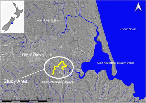
The Heathcote/Ōpāwaho is a spring-fed, lowland waterway with an average base flow of approximately 1 cumec (White et al. 2007). Riparian vegetation species in the study area included pasture grasses such as tall fescue (Schedonorus arundinaceus) and creeping bent (Agrostis stolonifera), together with herbs such as monkey musk (Erythranthe guttata), watercress (Nasturtium officinale) and mint (Mentha spp.). Small stands of rāupo (Typha orientalis) and kuawa (Schoenoplectus tabernaemontani) were also present, generally at slightly lower elevations than īnanga spawning habitat and often emergent in the main channel. Other indigenous plant species were scarce, but included rushes (Juncus spp.), occasional sedges (e.g. Carex secta) and harakeke (Phormium tenax). The invasive exotic reed canary grass (Phalaris arundinaceae) was widespread throughout the study area in the īnanga spawning habitat elevation range. Infestations of Glyceria maxima were also present downstream. Oioi (Apodasmia similis) became more common near the downstream limit of the study area along with saltmarsh ribbonwood (Plagianthus divaricatus) and other saltmarsh species.

Establishing the survey area

During the December 2014 and January 2015 new moon spring tide sequence, the upstream extent of saltwater intrusion was determined using a hand-held salinity meter (YSI Model 30, YSI Inc., USA). The progression of the flood tide was followed upstream as described in Richardson and Taylor (2002) but using kayaks. Measurements were taken 10 cm from the bottom and top of the water column at locations recorded with GPS. Three conductivity/temperature loggers (Odyssey, Dataflow Systems Ltd, NZ) were deployed over the spring tide sequence with each logger secured 10 cm above the riverbed. The loggers were deployed near the upstream limit of salt water, near the saltmarsh vegetation transition zone (downstream), and at an intermediate position. Logger data were used to verify the peak salinity intrusion days across the tidal cycle while interpreting the hand-held meter data.

The upstream margin of the survey area was set 500 m upstream of the 0.2 ppt saline intrusion peak based on all measurements. This was interpreted as the upstream limit of seawater in the Heathcote/Ōpāwaho because a 0.1 ppt measurement was consistently recorded for >2 km further upstream. The downstream extent was set at the transition to dominant saltmarsh vegetation which is considered to be unsuitable for spawning (Mitchell and Eldon 1991). In the Heathcote/Ōpāwaho this transition is subtle, but this is not the case in all rivers. These steps resulted in the selection of a c. 4 km reach for surveying (Figure 1).

Detection of spawning sites

To achieve coverage of the entire survey reach within time restrictions, areas of potential habitat were first identified in a subjective survey similar to the expert judgement approach of Hicks et al. (2010), but using set criteria to define areas of high, moderate and poor quality habitat (Table 1). All areas of moderate and high quality habitat were surveyed systematically to detect egg occurrence. For each 5 m length of riverbank, three egg searches were completed at random locations at least 1 m apart. This resulted in a large number of independent searches. Each search involved inspecting the stems/tillers and root mat of riparian vegetation along a transect that ran perpendicular to the high-water mark. A 0.5-m wide and 2 m long swathe was inspected (1 m either side of the high-water mark). Where īnanga eggs were found the search area was extended by at least 50 m either side of the last occurrence to confirm the full extent of spawning.

Table 1. Īnanga spawning habitat quality classes and criteria.

Class	Quality of habitat for supporting spawning	Expected egg mortality rate	Criteria
1	Poor	High	Vegetation cover <100% or Stem density <0.2 cm^−2
2	Moderate	Moderate	Vegetation cover 100% Stem density >0.2 cm^−2 Aerial root mat depth <0.5 cm
3	High	Low	Vegetation cover 100% Stem density >0.2 cm^−2 Aerial root mat depth >0.5 cm

When quantifying spawning habitat, mortality of eggs between spawning and the survey is a potential confounding factor (Hickford and Schiel 2011b). To minimise this, a standardised schedule was used to improve comparability between months (Table 2). Surveys commenced six days after the peak tide sequence each month. Four to five days of surveying were required each month using a team of three people. Surveys took longer when more spawning was found.

Table 2. Tidal cycle data and survey periods for the 2015 Heathcote/Ōpāwaho survey.

Month of spawning	Peak tidal cycle start	Peak tidal cycle end	Lunar phase	Peak tidal height^a (m)	Survey period
February	22/2/2015	25/2/2015	New moon	2.6	March 3–6
March	20/3/2015	23/3/2015	New moon	2.6	March 29–April 3
April	18/4/2015	20/4/2015	New moon	2.6	April 26–30
May	17/5/2015	19/5/2015	New moon	2.6	May 26–30

^apredicted tide levels at Port of Lyttelton (Lat. 43° 36′ S Long. 172° 43′ E) in metres above Chart Datum (Source: LINZ).

Spatial data

Spawning ‘sites’ were defined as continuous or semi-continuous patches of eggs with dimensions defined by the pattern of occupancy. For all sites, the upstream and downstream extent of the site were established, coordinates recorded and length measured. The width of the egg band was measured at the centreline of the search transects falling within the site (minimum of three, adding additional transects where needed). Zero counts were included where they occurred (i.e. at discontinuous sites). Mean width of the egg band was calculated for each site. AOO was calculated as length × mean width. For temporal analysis, spawning was considered to occur at the same ‘site’ where the AOO overlapped between months.

Spawning site productivity

Productivity of each site was assessed by direct eggs counts using a sub-sampling method adapted from Hickford and Schiel (2011a). For each transect, a 10 × 10-cm quadrat was placed in the centre of the egg band and all eggs within the quadrat counted. For atypical locations where the egg patch was not a narrow band (e.g. in low bank gradient areas) a 1 m² grid was overlaid on the site and a 10 × 10-cm quadrat sampled at the centre of the egg band within each grid. This improved sampling spread along the vertical bank profile. For quadrats with very high egg densities (>200 quadrat⁻¹), egg numbers were estimated by further sub-sampling using five randomly located 2 × 2-cm quadrats and the average egg density of these sub-units used to estimate egg density for the larger 10 × 10-cm quadrat. Mean egg density was calculated from all 10 × 10-cm quadrats sampled within the site. Productivity was calculated as mean egg density × AOO.

Results

Habitat quality assessment

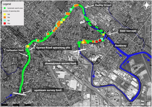
Within the study area, over 1.5 km of the true right bank was assessed as having high or moderate quality and was selected for egg surveys (Figure 2). These areas were not contiguous being spread out over a ca. 4 km reach extending from above the known spawning site near Opawa Road to near the downstream limit of the survey area. Habitat quality was assessed as poor for a large proportion of the true left bank as a result of steep bank profiles (often vertical) and erosion in the vicinity of the spring tide high-water mark with typically sparse vegetation. Only small sections supporting more established riparian vegetation were selected for egg surveys with the exception of a contiguous reach of c. 500 m near the downstream limit of the study area (Figure 2). The reach between Radley Street and the tidal barrage offered mostly poor habitat quality on both banks with tall trees limiting the amount and density of understorey vegetation in the riparian zone.

Figure 2. Areas subject to systematic egg searches and locations of spawning sites detected in each month (February–May) of the survey. The upstream limit of salt water (as measured) is also shown.

Egg surveys

Thirty-two spawning sites were identified over the four month survey period distributed over a reach of approximately 2.5 km with the upstream extent being Opawa Road (Figure 2). All spawning was found in ‘high’ quality habitat validating the habitat quality classification (Table 1). The number of spawning sites detected varied considerably between months with nine found in February, 27 in March, 27 in April, and six in May (Figure 2). Repeated use of the same area of riparian vegetation was observed at some sites, but other sites were used only once. Of the 27 sites found in 24 March were re-used in April, but the AOO often differed. Six sites (19%) were used only once, 23 sites (69%) twice, and 4 sites (12%) 3 times, with no site used on all 4 months of the survey.

AOO showed a defined peak in March (57.7 m² ± 2.7;  ± SE) (Figure 3A). Very little spawning was recorded in May (1.4 m² ± 0.2). The productivity peak was also in March with 3.3 × 10⁶ eggs recorded (Figure 3B), three times that of the next highest month (April). Total egg production over all months was 4.93 × 10⁶ ± 0.44 × 10⁶ eggs. Areas of occupancy varied considerably across the study area with large areas found a long distance apart (Figure 4A). The largest area was 13.3 m² recorded in February and in general not all sites were used in all months. Using the maximum AOO recorded at each of the 32 sites over all months, the cumulative AOO of spawning habitat utilised at least once was 74.6 m². The spatial distribution of egg production (Figure 4B) often reflected the AOO of spawning sites but also showed evidence of highly variable egg densities. The highest mean density was 13.5 eggs cm⁻² near Opawa Road, but >10 eggs cm⁻² were also recorded at two other sites. The average mean egg density across all spawning sites and months was 2.9 eggs cm⁻² ± 0.71.

Figure 3. Comparison of monthly totals for īnanga spawning site metrics in the Heathcote/Ōpāwaho catchment in 2015. A, Total area of occupancy. B, Total egg production. Each month represents the new moon spawning event. Error bars reflect standard errors of the mean for sub-sampled metrics at each site.

Figure 4. Īnanga spawning site metrics binned into contiguous 100 m reaches across the study area for each of the four months surveyed. A, Total area of occupancy. B, Total egg production. Assignment to bins was based on the centrepoint of each spawning site. Error bars reflect standard errors of the mean for sub-sampled metrics at each site. The full extent of the survey reach has been truncated for clarity.

Discussion

Application of the census approach has improved knowledge of īnanga spawning habitat in several ways. In particular, the Heathcote/Ōpāwaho example identified many previously unknown spawning sites in a well-studied catchment. This is notable because the literature has often reported the use of the same spawning sites year after year and this may simplify their protection and management (Richardson and Taylor 2002). However, there were also many more spawning sites than ever previously reported and they collectively occupied a much greater area. For example, the AOO has historically been in the order of 21 m² (Taylor 2002). In comparison, the area of spawning habitat used at least once in 2015 was 74.6 m². Potential reasons for the discrepancy between our results and previous estimates for the catchment include (i) exceptionally high numbers of spawning īnanga in 2015 when we undertook our survey and/or (ii) that previous survey efforts were not extensive or intensive enough to capture the full pattern. In addition, if the pre-earthquake spawning habitat had included degraded areas, the discovery of spawning sites in those areas would have been difficult due greater egg mortality (Hickford and Schiel 2011b), especially in sporadic surveys. Bank slumping and other effects of the earthquakes may have increased the availability of high quality habitat and in turn made detection more likely (Orchard and Hickford 2016).

The literature on īnanga spawning site ecology suggests that most spawning is found close to the upstream limit of the saltwater wedge associated with high tides (Richardson and Taylor 2002). In an analysis of the National Īnanga Spawning Database, Taylor (2002) calculated a median distance of 107 m between the location of spawning sites and the saltwater wedge position from all available data where both had been recorded (n = 84), although a few studies showing anomalies to this trend were identified. In Australia, Hicks, Barbee, Swearer and Downes (2010) reported spawning site distributions spanning several kilometres in some rivers although the saltwater limit position was not reported. In the Heathcote/Ōpāwaho, we consistently detected spawning habitat over 3 km downstream from the saltwater limit.

The census approach initially assumes that an extensive reach of the river may be capable of supporting īnanga spawning. Investigations are required to determine the actual reach to be surveyed. These focus on the saltmarsh vegetation transition (downstream) and the saltwater limit (upstream) on high tides. As was the case in our example, some judgement may be required in setting the downstream survey limit if there is a wide transition zone before salt marsh vegetation becomes dominant. However, due to the effect of river engineering works over many years the Heathcote/Ōpāwaho is a relatively complex example and the transition zone is typically more clear-cut in other rivers. In general, the downstream survey limit can be set to include all potential spawning habitat based on vegetation condition until at least such time as the peak spawning month has been identified. The pattern of spawning observed on peak months may assist decisions on whether to exclude some reaches in future surveys to reduce the survey effort.

Although a similar rationale may be applied to setting the upstream limit of the survey area, a pragmatic decision on the cut-off point will be required if the vegetation appears suitable for a long distance upstream. We chose a point 500 m upstream of the saltwater limit consistent with Richardson and Taylor (2002). Determining the saltwater limit is a crucial step and it is important that the field methodology is appropriate. We used data loggers to confirm the date(s) of maximum saltwater intrusion during the spring tide cycle on which spawning occurred. This provided a degree of validation for the salinity characterisation method using hand-held meters, which was only applied to one or two tides. Should a data logger be unavailable, we believe the salinity characterisation could also be reliably conducted by careful attention to the predicted peak tides and the possible influence of river flows when planning the field salinity measurements. The measurements should be taken on the largest tides and with low river flows to increase the chance that they will capture the maximum saltwater intrusion over the period when spawning may have occurred.

Once the survey limits were established we used a subjective habitat assessment to identify areas for intensive searches similar to Hicks, Barbee, Swearer and Downes (2010). However, a key aspect of our approach is the use of set criteria to guide the identification of potentially important areas. The Heathcote/Ōpāwaho study shows that the criteria and thresholds chosen were useful in refining the search area with no evidence that spawning sites were missed through their application. This aspect helps improve the repeatability of the survey methodology in practice.

Attention to temporal replication is a further defining feature of our census survey approach. Between-month comparisons in the Heathcote/Ōpāwaho show that the distribution and number of spawning sites varied considerably despite the repeat use of some sites. AOO comparisons show major differences in the area occupied each month further highlighting the importance of temporal replication when quantifying spawning habitat. March spawning exceeded February by a factor of three in the number of sites and their combined AOO. As exemplified by the March–April comparison, the AOO can vary markedly even with the same number of spawning sites being used. These findings suggest that the number of monthly surveys and seasonal timing aspects are critical considerations.

Where temporal trends are of interest there is a practical necessity to discover all of the spawning sites. For egg production this may be especially crucial due to the influence of varying egg densities. In this study, the average egg densities per site varied by up to three orders of magnitude (i.e. from 10² to in excess of 10⁵ eggs m⁻²). There were many examples of relatively large sites with low egg densities whereas several small sites had very high egg densities and contributed greatly to total production in the catchment. Very few studies have quantified egg numbers, especially on a catchment basis, and we are not aware of any studies that have quantified spatio-temporal variation in patterns of egg production. However, the failure to detect high density sites is potentially a key issue. Our census survey methodology provides a comprehensive and replicable means to address spatio-temporal variation.

Lastly, the Heathcote/Ōpāwaho study identified a high proportion of the total spawning at sites where reed canary grass (P. arundinaceae) was the dominant vegetation. Spawning has not previously been recorded on this invasive species and other studies have identified it as a threat and recommended removal (Taylor 2002; Taylor and Chapman 2007). The control of reed canary grass is certainly more complex in light of this finding. However, it may be possible to undertake a staged approach to reed canary grass removal guided by regular monitoring of egg production and habitat occupancy.

Taken together these findings suggest that the census survey methodology can make a useful contribution to habitat management. It may assist integration with other land uses by more precisely informing tools such as spatial planning. Monitoring applications include the evaluation of habitat protection initiatives and trends in egg production.

Conclusions

Our aim was to develop a survey methodology that can determine the full extent of īnanga spawning habitat within a river system. This information is lacking in most of New Zealand’s river systems and will improve the implementation of current conservation policy. Although the survey effort is considerable, the Heathcote/Ōpāwaho example shows that it can be readily applied to a large study area. Limitations include the availability of sufficient personnel. There is a practical necessity for completion before the hatch date and egg mortality rates introduce an additional confounding factor, especially at degraded sites. Completing the survey within a standardised time frame relative to the date of spawning is important to improve the comparability of repeated surveys at the same study site. Practical strategies for larger sites include increasing the number of researchers and the potential use of volunteers. Results gained in this first application of the methodology confirm its utility and underlying rationale. The findings suggest that spatio-temporal variability in spawning combined with the timing and extent of surveys have the potential to exert large effects on the results, directly influencing the inference that can be draw from them.

Acknowledgements

We thank Jesse Burns, Jason Telford, Nicole Wehner, Eimear Egan, and Judith Rikmanspoel for assisting with field surveys, and the staff of the Waterways Centre for Freshwater Research and Marine Ecology Research Group for support.

Disclosure statement

No potential conflict of interest was reported by the authors.

ORCID

Shane Orchard http://orcid.org/0000-0002-9040-6404

Michael J. Hickford http://orcid.org/0000-0002-0275-6632

Additional information

Funding

This work was supported by the Ngāi Tahu Research Centre, IPENZ Rivers Group and a New Zealand Ministry for Business Innovation and Employment: [Grant Number C01X1002].

References

- Burnet AMR. 1965. Observations on the spawning migrations of Galaxias attenuatus. New Zealand Journal of Science. 8:79–87.
- Goodman J. 2016. New Zealand whitebait fishery. Report prepared for New Zealand conservation authority, 22 November 2016. DOCCM-2922143. 125-139.
- Goodman JM, Dunn NR, Ravenscroft PJ, Allibone RM, Boubée JAT, David BO, Griffiths M, Ling N, Hitchmough RA, Rolfe JR. 2014. Conservation status of New Zealand freshwater fish, 2013. New Zealand threat classification series. Wellington: Department of Conservation; p. 12.
- Hickford MJH, Cagnon M, Schiel DR. 2010. Predation, vegetation and habitat-specific survival of terrestrial eggs of a diadromous fish, galaxias maculatus (Jenyns, 1842). J Exp Mar Biol Ecol. 385:66–72. doi: 10.1016/j.jembe.2010.01.010
- Hickford MJH, Schiel DR. 2011a. Population sinks resulting from degraded habitats of an obligate life-history pathway. Oecologia. 166:131–140. doi: 10.1007/s00442-010-1834-7
- Hickford MJH, Schiel DR. 2011b. Synergistic interactions within disturbed habitats between temperature, relative humidity and UVB radiation on egg survival in a diadromous fish. PLoS ONE. 6:e24318. doi: 10.1371/journal.pone.0024318
- Hicks A, Barbee NC, Swearer SE, Downes BJ. 2010. Estuarine geomorphology and low salinity requirement for fertilisation influence spawning site location in the diadromous fish, Galaxias maculatus. Marine and Freshwater Research. 61:1252–1258. doi: 10.1071/MF10011
- Kennish MJ. 2002. Environmental threats and environmental future of estuaries. Environ Conserv. 29:78–107. doi: 10.1017/S0376892902000061
- McDowall RM. 1984. The New Zealand whitebait book. Wellington: Reed.
- Mitchell CP. 1994. Whitebait spawning ground management. New Zealand Department of Conservation, Science and Research Series. 69:1–23.
- Mitchell CP, Eldon GA. 1991. How to locate and protect whitebait spawning grounds. Rotorua: Freshwater Fisheries Centre; p. 49.
- Orchard S, Hickford M. 2016. Spatial effects of the Canterbury earthquakes on īnanga spawning habitat and implications for waterways management. Report prepared for IPENZ rivers group and Ngāi Tahu Research Centre Waterways Centre for Freshwater Management and Marine Ecology Research Group. Christchurch: University of Canterbury; p. 37.
- Richardson J, Taylor MJ. 2002. A guide to restoring inanga habitat. NIWA Science and Technology Series. 50:1–29.
- Taylor MJ. 2002. The national inanga spawning database: trends and implications for spawning site management. Science for Conservation 188. Wellington: Department of Conservation; p. 37.
- Taylor MJ, Chapman E. 2007. Monitoring of fish values; inanga and trout spawning. AEL Report No. 54. Christchurch: Aquatic Ecology Limited; p. 22.
- White PA, Goodrich K, Cave S, Minni G. 2007. Waterways, swamps and vegetation of Christchurch in 1856 and baseflow discharge in Christchurch city streams. GNS Science Consultancy Report 2007/103. Taupo: GNS; p. 81.