Acoustically estimated size distribution of sperm whales (Physeter macrocephalus) off the east coast of New Zealand

ABSTRACT

The length-frequency distribution of sperm whales (Physeter macrocephalus) was studied on the east coast of NZ using passive acoustic recorders moored offshore of Kaikoura, Cape Palliser and Castlepoint. Sperm whale’s echolocation signals are unique among odontocete species. Their clicks are composed by multiple pulses resulting from the sound transmission within the whale head. The total length of the whales can be estimated by measuring the time delay between these pulses. A total of 997 length measurements were obtained from click trains using cepstral analysis (mean = 14.6 m; min = 9.6 m; max = 18.3 m; std = 1 m). The size-frequency distributions at all three locations were similar, although animals smaller than 12 m were not present offshore of Kaikoura. Animals of various sizes appeared to be present all year round, with no apparent seasonality in the occurrence of any size class.

KEYWORDS:

• Passive acoustics
• PAM
• sperm whale
• length-frequency distribution
• ceptrum
• cepstral analysis
• echolocation
• marine mammal
• odontocete

Introduction

Sperm whales (Physeter macrocephalus) are unique among marine echolocating species; their vocal repertoire consists of click sounds that are usually produced in different patterns for different behaviors. For example, sperm whales produce stereotyped series of clicks called ‘codas’ when socialising that appear to vary geographically (Weilgart and Whitehead 1997; Rendell and Whitehead 2003). Sperm whales also produce echolocation clicks at regular intervals in long series during foraging dives to find prey (Jaquet et al. 2001; Madsen et al. 2002; Fais et al. 2015). These signals are characterised by a repetition rate (referred to as inter-click-interval or ICI) ranging between approximately 0.5 and 2 s (Zimmer et al. 2005a), a centroid frequency of ∼15 kHz and a source level of up to 236 dB re 1 µPa (rms) (Møhl et al. 2003a). Finally, sperm whales are also known to produce high repetition rate echolocation clicks, referred to as ‘creaks’ or ‘buzzes’ that are associated with prey capture during foraging dives (Miller et al. 2004).

The peculiarity of the sperm whale echolocation click is its multi-pulsed structure (Backus and Schevill 1966), a result of a sound generation process that can produce clicks as long as 30 ms (Møhl et al. 2003a; Møhl et al. 2003b). Norris and Harvey (1972) were the first to propose an explanation to this phenomenon. They suggested that the sound is generated by the phonic lips; the main pulse (called p1) propagates in front of the head and subsequent pulses (called p2, p3 etc.) are generated by the reverberation of sound that back-propagates into the head and reflects off two air sacs located at both sides of the spermaceti organ (Norris and Harvey 1972). This sound generation model was successively modified when the existence of a low amplitude pulse (called p0) preceding p1 was discovered and the sound transmission inside the whale’s head was tested (Møhl and Amundin 1991; Møhl 2001). The updated model (known as the bent-horn model) proposed that the sound generated by the phonic lips is mainly directed backward into the spermaceti organ, with some energy propagating forward and generating the p0 pulse. The backward-propagating soundwave is reflected forward by the frontal air sac, then travels forward through the ‘junk’ organ and exits the nose of the whale as p1 pulse. Successive pulses (p2, p3 etc.) are generated by sound reflections between the distal and the frontal air sacs (Zimmer et al. 2005a). As a result, the time difference between pulses (referred to as inter-pulse-interval, or IPI) is proportional to the length of the head.

Since the allometric relationship between the nasal complex and the total body length of sperm whale is known from whaling studies (Nishiwaki et al. 1963), an empirical method to estimate the length of sperm whale by measuring IPI within the click was developed (Gordon 1991) based on known measurements of sound speed in the spermaceti organ (Flewellen and Morris 1978). This method was later validated in stranded animals through body and nasal complex length measurements (Møhl 2001), and subsequently tested using photogrammetry in wild sperm whales (Dawson and Slooten 1995; Rhinelander and Dawson 2004), and led to the development of equations that better fit length data for larger individuals (Rhinelander and Dawson 2004; Growcott et al. 2011).

A precise measurement of the IPI is critical for estimating sperm whales length from their echolocation clicks. Goold (1996) compared the performance of two signal processing techniques; waveform cross-correlation and cepstrum analysis and found that the variability of signal quality was unreliable for both techniques when applied to a single click. However, computing the IPIs for several hundred clicks and smoothing the result using a moving average produced realistic results (Goold 1996). Variability in IPIs of the same individual has been documented (Rhinelander and Dawson 2004; Bøttcher et al. 2018). Rhinelander and Dawson (2004) found a statistical difference in the IPI measured during sperm whales dives within the same day, but concluded that such a difference was small in magnitude, leading to a length estimation error <3%. In a more recent study, Bøttcher et al. (2018) used data from an acoustic tag to study the variability of IPIs within individuals. They proposed that the observed variation (approximately 0.2 ms) could be explained by the dynamics of the soft structure of the sperm whale nose. Off-axis effects also affect IPIs measurements. Zimmer et al. (2005b) described the effect of the whale orientation on IPIs by combining acoustic recordings from tags and far-field recordings from a line array of hydrophones. This study showed that IPI can be measured from clicks recorded in front or behind the whale, but when recorded at an off-axis angle, the pulses within the click are not evenly spaced and, therefore, not useful for IPI estimation (Zimmer et al. 2005b).

A solution to overcome the uncertainties in IPI measurements consists of averaging a large number of cepstra (Bogert et al. 1963) of echolocation signals produced by the same whale (Teloni et al. 2007). This methodology produces a consistent estimation of the spermaceti organ both in the case of unknown whale orientation and when recordings are affected by surface reflections (Teloni et al. 2007). In addition, studies have found that consistent IPI values are obtained by averaging cepstra of ∼50 clicks (Antunes et al. 2010).

In this paper, the techique described by Teloni et al. (2007) was applied to a-year long dataset of sperm whale echolocation activity recorded along the eastern coast of New Zealand to estimate the size of sperm whales that forage in the study area. This tecqnique has been used to estimate the size-frequency distribution of sperm whales recorded in 2005 with the NEMO-OνDE cabled observatory in the Mediterranean sea (Caruso et al. 2015). This is the first study to apply cepstral analysis to passive acoustic recordings collected year-round at multiple distant locations in New Zealand waters.

Methods

Data collection

Acoustic data were collected using three Autonomous Multichannel Acoustic Recorders (AMAR; JASCO Applied Sciences, Dartmouth, Canada) each equipped with an M36-V35-100 omnidirectional hydrophone (GeoSpectrum Technologies Inc.) with a relatively flat frequency response (±3 dB re 1 V/μPa) between 100 Hz and 80 kHz and a sensitivity of −164 dB re 1 V/μPa. The recorders were moored to the bottom of the ocean east/southeast of Cook Strait in water depths >1000 m (Figure 1). The AMARs operated on a duty cycle, recording 125 s every 15 min at a sampling rate of 250 kHz. The recorders were deployed 6–7 June 2016, serviced December 2016–February 2017, re-deployed 21–23 February 2017, and recovered between 30 August and 8 September 2017 (Table 1).

Figure 1 . Location of the 3 acoustic recorders (red pin symbols) in the study area. For consistency with Giorli and Goetz (2019), station A will be referred to as ‘Kaikoura’; Station B will be referred to as ‘Palliser’; Station C will be referred to as ‘Castlepoint’.

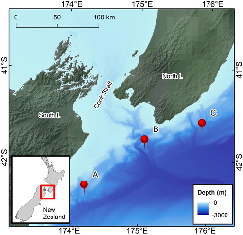
Table 1. Position and details of the recorders.

Station	Deployment date	Re-deployment date	Last recording	Depth (m)	Latitude (decimal degrees)	Longitude (decimal degrees)
Kaikoura ‘A’	7 June 2016	22 February 2017	8 September 2017	1250	−42.3087	174.2145
Palliser ‘B’	6 June 2016	21 February 2017	30 August 2017	1290	−41.8050	175.0810
Castlepoint ‘C’	6 June 2016	23 February 2017	30 August 2017	1480	−41.6098	175.9029

Notes: Dates are reported in UTC time.

Echolocation click detection

A custom-made MATLAB (Mathwork Inc., Natick, Massachusetts, USA) algorithm was developed to detect and classify sperm whale’s echolocation click trains (Giorli and Goetz 2019). A sixth order band-pass filter (cut off frequencies of 2 and 20 kHz to include sperm whale’s echolocation signals bandwidth (Møhl et al. 2003a; Zimmer et al. 2005a; Caruso et al. 2015)) was applied to the acoustic data. Click trains were detected in the filtered data using an adaptive threshold that self-adjusted to 4 dB above the average noise level in each wav file recorded. Inter Click Intervals (ICI), duration (time between the 5th and 95th of the signal energy), and peak frequency of each signal detected above the threshold were measured. Individual click trains were isolated by grouping echolocation clicks with ICI< than 3 s between consecutive signals. Click trains containing less than 5 echolocation signals were eliminated from further analysis.

The probability of each click-train of being produced by a sperm whale was computed by dividing the number of clicks that meet the requirements for peak frequency, ICI and duration by the total number of echolocation signals in the click train. A click train was considered to be from a sperm whale if this probability was higher than 70%.

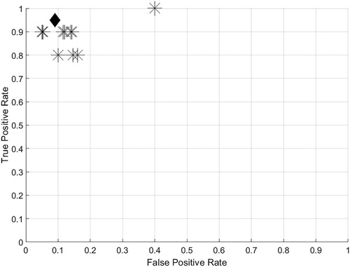
The ranges for the peak frequency, ICI, and duration were adjusted using a training dataset composed of 100 .wav files that did not contain sperm whale echolocation signals (although they did contain noise from boats, echosounders, and echolocation signals from other odontocete species), and 100 .wav files that contain sperm whale echolocation signals (although they also contained noise from boats, echosounders, multiple sperm whales echolocating at the same times, and echolocation signals from other odontocete species). The training dataset was composed of 125 s long .wav files recorded during this study using AMARs. This dataset was developed by an experience researcher that visually screened the data. Thirteen different algorithm performance tests (with varying ranges for peak frequency, ICI and signal duration) were run on the training dataset and the detection/classification performance of each run was assessed using a Receiver-Operator Characteristic (ROC) approach. The false positive and true positive rates were calculated for each training trial (Figure 2) by comparing the algorithm results against the real occurrence of click trains in the training dataset. The probability of correct response (Egan 1975; Au and Hastings 2008) using the selected ranges was 0.9. After the training, the selected ranges were 4 to 15 kHz for peak frequency; 0.2 to 2 s for ICI; and 500 to 1200 µs for signal duration. Previous research used such an approach of classifying click trains (Giorli et al. 2016a, 2016b; Giorli and Goetz 2019). A 40 ms long pressure time series around each echolocation signal in each click train detected was extracted. This time frame was chosen in order to capture both the p1 and p2 pulses required for size estimation (Teloni et al. 2007; Caruso et al. 2015).

Figure 2. (From Giorli and Goetz 2019). True and false positive rates from the detection algorithm training trials (n = 13). The value of the trial selected is indicated by the ‘♦’ symbol. The probability of correct response (Egan 1975; Au and Hastings 2008) of the trial indicated by the ‘♦’ was 0.9. Plotting clarity was improved by jittering the data.

Length estimation

The length of the detected sperm whales was estimated using the methodology described by Teloni et al. (2007), which was also applied to passive acoustic data collected in the Mediterranean Sea (Caruso et al. 2015). Only click trains containing more than 50 clicks were used for length estimation (Antunes et al. 2010; Caruso et al. 2015). The stable IPIs (Zimmer et al. 2005b) were measured by computing the cepstra’s gamnitude C of each echolocation signal (Teloni et al. 2007) as follows:$C=\left|FF{T}^{-1}\left(\text{log}\left|FFT\left(\left|x^2\right|\right)\right|\right)\right|$where x is the 40 ms long pressure time-series extracted by the detection algorithm around each echolocation click detected in the click train. The cepstra contained in each click train were averaged and the mean IPI was obtained by computing the maximum gamnitude between the quefrency of 2 and 11 ms of the averaged cepstra (Goold 1996; Caruso et al. 2015). This method assumes that the echolocation signals in each click train analysed are produced by the same individual. All averaged cepstra were visually inspected by an experienced operator, and those that did not contain a clear peak in gamnitude were discarded. Selected cepstra had a gamnitude peak width ≤1 ms, as described in Miller et al. (2013). Autocorrelation in the data was reduced by excluding an IPI from further analysis if (1) it occurred within 2 h from the previous one and (2) it differed less than 0.3 ms from the previous measurement (as indicated in Bøttcher et al. 2018). Potential outliers were removed from the data using the Interquartile Range method. An IPI measurement was considered an outlier if its value was 1.5 interquartile ranges above the upper quartile or below the lower quartile.

The measured mean IPI was then used to estimate the size of the sperm whale producing the click train using the following equations (Gordon 1991; Growcott et al. 2011):(1) $BodyLength=4.833+1.453\times IPI-0.001\times IP{I}^2;$(1) (2) $BodyLength=1.258\times IPI+5.736;$(2)

Gordon (1991) derived his equation from photogrammetry measurements of 11 animals (ranging between ∼9.5 and ∼10.5 m in length; only one animal longer than 12 m). Growcott et al. (2011) deducted his formula using photogrammetry data and IPIs of 33 sperm whales longer than 12 m (∼5 ms IPI). Gordon’s formula is well suited for measurements of individuals < 11 m (∼ 4 ms IPI); while Growcott’ equation better fits the measurement of larger individuals (IPI > 4 ms; Caruso et al. 2015).

Results

Approximately 7 TB of acoustic data was collected (∼2.3 TB at Castlepoint; ∼2.4 TB at Kaikoura; ∼ 2.2 TB at Palliser) for a total of 113,608 125 s long .wav files recorded (37,521 at Castlepoint; 38,404 at Kaikoura; 37,683 at Palliser). The dataset produced by the detection algorithm consisted of 4,897 sperm whales click trains (see Figure 3 for example), each containing more than 50 echolocation clicks (2,641 at Kaikoura; 918 at Castlepoint; 1,338 at Palliser). After visual inspection of the averaged cepstra, 1,551 click trains showed a clear peak in the gamnitude (Figure 4). After removing both ceptra that did not satisfy the autocorrelation condition and outliers, a total of 997 click trains were used to calculate body length (250 at Palliser; 586 at Kaikoura; 161 at Castlepoint). IPIs measurements ranged between 3.3 and 10 ms (mean IPI = 7 ms; std = 0.86 ms).

Figure 3. Example of a click train with more than 50 clicks recorded at the Castlepoint location on 07/06/2016 at 05:10 am (UTC time). Relative amplitude in time domain is shown on the top and the respective spectrogram on the bottom.

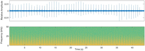
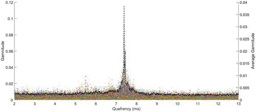
Figure 4. Example of individual click cepstra (coloured points) and their average cepstra (black dashed line) for the sperm whale click train showed in Figure 3. The resulting maximum averaged gamnitude is at the quefrency is 7.38 ms, corresponding to a body length of about 15 m (Growcott et al. 2011).

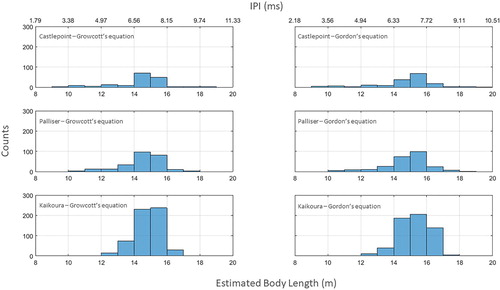
The size-frequency distributions computed with the two different equations at all three locations were very similar (Figure 5). All distributions were not normal (Kolmogorov–Smirnov test; p < 0.05). Most of the sperm whales click trains were estimated to be produced by individuals between 14 and 16 m in length, although smaller individuals (< than 12 m) were also present at the Castlepoint and Palliser stations. Very few (n = 3) click trains were estimated to be produced by individuals larger than 18 m, regardless of the equation used to calculate length.

Figure 5. General size frequency distributions derived from IPIs at the Castlepoint (top panel), Palliser (middle panel) and Kaikoura (bottom panel) locations, using Growcott’s equation (left panel) and Gordon’s equation (right panel).

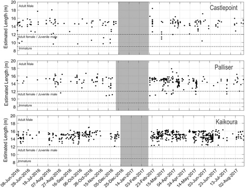
There was no evidence of a temporal trend in body length (Figure 6). At all locations, animals of various sizes appeared to be present all year round, with no apparent seasonality in the occurrence of any size class. However, it is possible that smaller animals occurred, but the AMARs did not record any click train longer than 50 clicks from these animals.

Figure 6. Body length estimates per day at the Castlepoint (top panel), Palliser (middle panel) and Kaikoura (bottom panel) locations. The data gap between the end of December 2016 and the end of February 2017 correspond to the period during which the recorders were not deployed. Estimated lengths are reported using Gordon’s equation for IPIs < 4 ms and Growcott’s equation for IPIs > 4 ms. Dashed lines indicate the hypothetical sex and sexual maturity as described in Caruso et al. (2015).

Discussion

This paper presents length-frequency distributions of sperm whales at three distinct locations along the East coast of New Zealand. Studies that examine the length-frequency distribution from acoustic monitoring programmes across seasons and years are valuable as they can provide information on population parameters, such as general growth rates, and changes on the population structure over time. Overall there is a good correspondence between our results and previous studies that estimated body length of sperm whales. Our passive acoustic monitoring approach for measuring sperm whales size-frequency distribution proved to be an effective way to monitor the size range and its temporal variability over a large spatial-temporal area of New Zealand waters.

The social structure and composition of sperm whale groups in New Zealand has been investigated using data collected during commercial whaling (Gaskin 1970; Gaskin and Cawthorn 1973), stranding events (Stephenson 1975) and ship-based surveys (Webb 1973). These studies reported the presence of solitary males, schools of bachelor males, immature individuals, and nursery schools. Adult males length was reported to range between 8 and 16 m, adult females between 8 and 12 m, immatures between 7 and 11 m, and calves between 4 and 8 m (Gaskin 1970; Gaskin and Cawthorn 1973; Webb 1973; Stephenson 1975). In particular, Gaskin and Cawthorn (1973) provided a length-frequency distribution based on measurements of 238 sperm whales caught between 1963 and 1964 by the Tory Channel Whaling Company. The histogram reported in their publication show peaks between ∼14 and ∼15 m (45 and 50 feet, n = 241) for male individuals, and ∼10.5 m for females (35–36 feet; n = 7). Additional data on sperm whale body length in New Zealand was collected around the Kaikoura peninsula with whale lengths estimated between 9.3 and 15.8 m for 12 individuals measured optically (Dawson and Slooten 1995) and between 12.5 and 15.3 m for 19 individuals measured acoustically (Rhinelander and Dawson 2004). These estimated lengths are similar to those of other studies that measured sperm whales in the same area (Growcott et al. 2011; Miller et al. 2013). Even though past studies demonstrated that juveniles and young animals are present around New Zealand (Gaskin 1970; Gaskin and Cawthorn 1973; Webb 1973; Stephenson 1975), recent research suggests that sperm whales in this region are primarily adults (Growcott et al. 2011; Miller et al. 2013). Animals estimated to be shorter than 11 m were considered as outliers by our data analysis method. However, there are uncertainties as to whether juveniles and immature animals are actually present in the area or if this is an artefact of data processing. A deeper understanding on the occurrence of immature and juveniles would allow for a better understanding of the sperm whale population structure in New Zealand.

Other studies have examined the size structure of sperm whale populations data collected from passive acoustic recorders. In the North Atlantic Ocean, estimates of sperm whale lengths ranged between 7 and 22 m for a total of 41 click trains (Adler-Fenchel 1980). Size measurements from the Northern Pacific Ocean were reported from whaling data (Ohsumi 1966) and show a bimodal distribution with peaks around 12.2 m (40 feet) and 14.9 m (49 feet) for caught whales (measured on board), and a normal distribution with a peak around 14.6 m (48 feet) for whales encountered during the study (estimated length). Another study of IPI-derived size structure of sperm whale population was conducted in the Mediterranean Sea (Caruso et al. 2015). The size of individual whales was measured over almost a year using data collected from an underwater cabled observatory. Furthermore, using estimated lengths, this study categorised each sperm whale by sex and maturity status using previously published growth rates (Rice 1989); most individuals were between 9 and 12 m (categorised as adult females or juvenile males), and only 13 whales were estimated between 12 and 14 m (categorised as adult males). In contrast, our measurements showed that the population of sperm whales in New Zealand is mostly comprised of individuals larger than the ones in the Mediterranean Sea, and mostly large males (if we adopt the same categorisation as Caruso et al. (2015)).

This study was able to measure the size of about a thousand click trains. However, limitations of this approach should be considered. As demonstrated in previous studies (Rhinelander and Dawson 2004; Bøttcher et al. 2018), IPIs show some variability in individual sperm whales. Although the size error associated with variability in IPI (<3% according Rhinelander and Dawson (2004); and in the order of 0.2–0.3 ms according to Bøttcher et al. (2018)) is small relative to the total length of mature sperm whales (± ∼0.30–0.43 m for Gordon’s equation, and ± ∼0.25–0.37 m for Growcott’s equation), results should be interpreted accordingly. Finally, it is not possible to reliably collect IPI data on small individuals including calves. An empirical equation to compute body length from cepstra for individuals shorter than ∼9 m does not exist. Moreover, clicks recorded from a captive neonate sperm whale did not appear to have the characteristic multi-pulsed structure typical of those produced by mature whales (Madsen et al. 2003).

Length-frequency distributions studies are routinely used to extrapolate growth rates in fisheries sciences (Francis and Francis 1992; Francis 1997), an essential aspect for determining maximum sustainable yields for commercially fished species, as well as information on many ecological aspects of a species (Smith et al. 1998), such as age, size at maturity, population structure and conservation status (Waters and Whitehead 1990). Cepstral analysis of sperm whale echolocation signals can be used to compute growth rates for this species if the same individuals can be recorded over the years (Miller et al. 2013). Hence, using passive acoustic technology and expanding its spatial and temporal coverage could allow to estimate the sperm whale population structure in New Zealand waters. However, the current methodology to estimate body length using the cepstral techniques is not reliable for small sperm whales and cannot distinguish between individuals. This prevents reliable measurement of animals across all age classes and may result in some individuals being measured multiple times. Size detection problems also exist when measuring size of other species such as fish. Using statistical methods, to estimate the size distribution in a fish population, the proportion of size classes or age classes retained by a fishing gear is accounted for in fisheries stock assessments (Maunder et al. 2014). Hence, combining techniques used in fisheries with acoustic estimations of sperm whales’ length might provide a way to investigate sperm whale’s population structure over a larger area.

Acknowledgements

The authors wish to thank the multiple sponsor of the project including OMV New Zealand Ltd, Chevron New Zealand Holdings LLC, Woodside Energy Ltd, and Marlborough District Council. We also would like to thank all the crew members and captains of the NIWA research vessels Tangaroa, Kaharoa, and Ikatere, as well as NIWA technicians Mike Brewer, Fiona Elliott, Sarah Searson, Olivia Price and Brett Grant for their help in constructing, deploying and recovering the moorings. Craig McPherson and Christopher Whitt from JASCO Applied Sciences were instrumental in mooring design and placement. Finally, we would like to acknowledge Marco Kienzle for its suggestions on fisheries modelling studies.

Disclosure statement

No potential conflict of interest was reported by the authors.

References

- Adler-Fenchel HS. 1980. Acoustically derived estimate of the size distribution for a sample of sperm whales (Physeter catodon) in the Western North Atlantic. Canadian Journal of Fisheries and Aquatic Sciences. 37(12):2358–2361. doi: 10.1139/f80-283
- Antunes R, Rendell L, Gordon J. 2010. Measuring inter-pulse intervals in sperm whale clicks: consistency of automatic estimation methods. The Journal of the Acoustical Society of America. 127(5):3239–3247. doi: 10.1121/1.3327509
- Au WW, Hastings MC. 2008. Principles of marine bioacoustics. New York (NY): Springer.
- Backus RH, Schevill WE. 1966. Physeter clicks. In: Norris KS, editor. Whales, dolphins, and porpoises. Berkeley (CA): University of California Press; p. 510–528.
- Bogert BP, Healy MJR, Tukey JW. 1963. The quefrency analysis time series for echoes: cepstrum, pseudoautocovariance, cross-cepstrum, and saphe cracking. In: Rosenblatt M, editor. Symposium on time series analysis. New York (NY): Wiley; p. 209–243.
- Bøttcher A, Gero S, Beedholm K, Whitehead H, Madsen PT. 2018. Variability of the inter-pulse interval in sperm whale clicks with implications for size estimation and individual identification. The Journal of the Acoustical Society of America. 144(1):365–374. doi: 10.1121/1.5047657
- Caruso F, Sciacca V, Bellia G, De Domenico E, Larosa G, Papale E, Pellegrino C, Pulvirenti S, Riccobene G, Simeone F, et al. 2015. Size distribution of sperm whales acoustically identified during long term deep-sea monitoring in the Ionian Sea. PloS One. December:1–16.
- Dawson SM, Slooten E. 1995. An inexpensive stereophotographic technique to measure sperm whales from small boats. Reports of the International Whaling Commissions. 45:431–346.
- Egan JP. 1975. Signal detection theory and ROC analysis. New York (NY): Academic Press.
- Fais A, Aguilar Soto N, Johnson M, Perez-Gonzalez C, Miller PJO, Madsen PT. 2015. Sperm whale echolocation behaviour reveals a directed, prior-based search strategy informed by prey distribution. Behavioral Ecology and Sociobiology. 69(4):663–674. doi: 10.1007/s00265-015-1877-1
- Flewellen CG, Morris RJ. 1978. Sound velocity measurements on samples from the spermaceti organ of the sperm whale (Physeter catodon). Deep Sea Research. 25(3):269–277. doi: 10.1016/0146-6291(78)90592-1
- Francis M. 1997. Spatial and temporal variation in the growth rate of elephantfish (Callorhinchus milii). New Zealand Journal of Marine and Freshwater Research. 31(1):9–23. doi: 10.1080/00288330.1997.9516741
- Francis MP, Francis RICC. 1992. Growth rate estimates for New Zealand rig (Mustelus lenticulatus). Marine and Freshwater Research. 43(5):1157–1176. doi: 10.1071/MF9921157
- Gaskin DE. 1970. Composition of schools of sperm whales physeter catodon linn. East of New Zealand. New Zealand Journal of Marine and Freshwater Research. 4(4):456–471. doi: 10.1080/00288330.1970.9515359
- Gaskin DE, Cawthorn MW. 1973. Sperm whales Physeter catodon L. in the Cook Strait region of New Zealand: some data on age, growth, and mortality. Norw. J. Zool. 21:45–50.
- Giorli G, Goetz KT. 2019. Foraging activity of sperm whales (Physeter macrocephalus) off the east coast of New Zealand. Scientific Reports. 9(1):1–9. doi: 10.1038/s41598-019-48417-5
- Giorli G, Neuheimer A, Au WWL. 2016a. Spatial variation of deep diving odontocetes’ occurrence around a canyon region in the Ligurian Sea as measured with acoustic techniques. Deep Sea Research Part I: Oceanographic Research Papers. 116:88–93. doi: 10.1016/j.dsr.2016.08.002
- Giorli G, Neuheimer A, Copeland A, Au WWL. 2016b. Temporal and spatial variation of beaked and sperm whales foraging activity in Hawai’i, as determined with passive acoustics. The Journal of the Acoustical Society of America. 140(4):2333–2343. doi: 10.1121/1.4964105
- Goold JC. 1996. Signal processing techniques for acoustic measurement of sperm whale body lengths. The Journal of the Acoustical Society of America. 100(5):3431–3441. doi: 10.1121/1.416984
- Gordon JC. 1991. Evaluation of a method for determining the length of sperm whales (Physeter catodon) from their vocalizations. Journal of Zoology. 224(2):301–314. doi: 10.1111/j.1469-7998.1991.tb04807.x
- Growcott A, Miller B, Sirguey P, Slooten E, Dawson S. 2011. Measuring body length of male sperm whales from their clicks: The relationship between inter-pulse intervals and photogrammetrically measured lengths. The Journal of the Acoustical Society of America. 130(1):568–573. doi: 10.1121/1.3578455
- Jaquet N, Dawson S, Douglas L. 2001. Vocal behavior of male sperm whales: Why do they click? The Journal of the Acoustical Society of America. 109(5):2254–2259. doi: 10.1121/1.1360718
- Madsen PT, Carder DA, Au WW, Nachtigall PE, Møhl B, Ridgway SH. 2003. Sound production in neonate sperm whales (L). The Journal of the Acoustical Society of America. 113(6):2988–2991. doi: 10.1121/1.1572137
- Madsen PT, Wahlberg M, Møhl B. 2002. Male sperm whale (Physeter macrocephalus) acoustics in a high-latitude habitat: implications for echolocation and communication. Behavioral Ecology and Sociobiology. 53:31–41. doi: 10.1007/s00265-002-0548-1
- Maunder MN, Crone PR, Valero JL, Semmens BX. 2014. Selectivity: theory, estimation, and application in fishery stock assessment models. Fisheries Research. 158:1–4. doi: 10.1016/j.fishres.2014.03.017
- Miller BS, Growcott A, Slooten E, Dawson SM. 2013. Acoustically derived growth rates of sperm whales (Physeter macrocephalus) in Kaikoura, New Zealand. The Journal of the Acoustical Society of America. 134(3):2438–2445. doi: 10.1121/1.4816564
- Miller PJO, Johnson MP, Tyack PL. 2004. Sperm whale behaviour indicates the use of echolocation click buzzes “creaks” in prey capture. Proceedings. Biological Sciences/The Royal Society. 271(1554):2239–2247. doi: 10.1098/rspb.2004.2863
- Møhl B. 2001. Sound transmission in the nose of the sperm whale Physeter catodon. A post mortem study. Journal of Comparative Physiology A. 187(5):335–340. doi: 10.1007/s003590100205
- Møhl B, Amundin M. 1991. Sperm whale clicks: pulse interval in clicks from a 21 m specimen. In: Sound production in odontocetes, with emphasis on the harbour porpoise, Phocoena phocoena [PhD thesis by Amundin, M.]. University of Stockholm, p. 115–125.
- Møhl B, Madsen PT, Wahlberg M, Au WWL, Nachtigall PE, Ridgway SH. 2003b. Sound transmission in the spermaceti complex of a recently expired sperm whale calf. Acoustics Research Letters Online. 4(1):19–24. doi: 10.1121/1.1538390
- Møhl B, Wahlberg M, Madsen PT, Heerfordt A, Lund A. 2003a. The monopulsed nature of sperm whale clicks. Journal of the Acoustical Society of America. 114(2):1143–1154. doi: 10.1121/1.1586258
- Nishiwaki M, Ohsumi S, Maeda Y. 1963. Change of form in the sperm whale accompanied with growth. Scientific Reports of the Whales Research Institute, Tokyo. 17: 1–17.
- Norris KS, Harvey GW. 1972. A theory for the function of the spermaceti organ of the sperm whale (Physeter catodon). In: Galler SR, Schmidt-Koenig K, Jacobs KGJ, Belleville RE, editors. Animal orientation and navigation. Washington, DC: NASA Special Publication; p. 397–417.
- Ohsumi S. 1966. Sexual segregation of the sperm whale in the North Pacific. Scientific Reports of the Whales Research Institute, Tokyo. 23:125.
- Rendell LE, Whitehead H. 2003. Vocal clans in sperm whales (Physeter macrocephalus). Proceedings of the Royal Society B: Biological Sciences. 270(1512):225–231. doi: 10.1098/rspb.2002.2239
- Rhinelander MQ, Dawson SM. 2004. Measuring sperm whales from their clicks: Stability of interpulse intervals and validation that they indicate whale length. The Journal of the Acoustical Society of America. 115(4):1826–1831. doi: 10.1121/1.1689346
- Rice DV. 1989. Sperm whale, Physeter macrocephalus. In: Ridgway SH, Harrison RJ, editor. Handbook of marine mammals. Vol. 4. Lodon (UK): London Academic Press; p. 177–233.
- Smith BD, Botsford LW, Wing SR. 1998. Estimation of growth and mortality parameters from size frequency distributions lacking age patterns: the red sea urchin (Strongylocentrotus franciscanus) as an example. Canadian Journal of Fisheries and Aquatic Sciences. 55(5):1236–1247. doi: 10.1139/f98-015
- Stephenson AB. 1975. Sperm whales stranded at muriwai beach, New Zealand. New Zealand Journal of Marine and Freshwater Research. 9(3):299–304. doi: 10.1080/00288330.1975.9515569
- Teloni V, Zimmer WMX, Wahlberg M, Madsen PT. 2007. Consistent acoustic size estimation of sperm whales using clicks. Journal of Cetacean Research and Management. 9(2):127–136.
- Waters S, Whitehead H. 1990. Population and growth parameters of Galapagos sperm whales estimated from length distributions. Reports of the International Whaling Commissions. 40:225–235.
- Webb BF. 1973. Cetaceans sighted off the west coast of the South Island, New Zealand, summer 1970 (note). New Zealand Journal of Marine and Freshwater Research. 7(1–2):179–182. doi: 10.1080/00288330.1973.9515465
- Weilgart L, Whitehead H. 1997. Group-specific dialects and geographical variation in coda repertoire in South Pacific sperm whales. Behavioral Ecology and Sociobiology. 40(5):277–285. doi: 10.1007/s002650050343
- Zimmer WMX, Madsen PT, Teloni V, Johnson MP, Tyack PL. 2005b. Off-axis effects on the multipulse structure of sperm whale usual clicks with implications for sound production. Journal of the Acoustical Society of America. 118(5):3337–3345. doi: 10.1121/1.2082707
- Zimmer WMX, Tyack PL, Johnson MP, Madsen PT. 2005a. Three-dimensional beam pattern of regular sperm whale clicks confirms bent-horn hypothesis. The Journal of the Acoustical Society of America. 117(3):1473–1485. doi: 10.1121/1.1828501