Automatic Differentiation in MetaPhysicL and Its Applications in MOOSE

Abstract

Efficient solution via Newton’s method of nonlinear systems of equations requires an accurate representation of the Jacobian, corresponding to the derivatives of the component residual equations with respect to the degrees of freedom. In practice these systems of equations often arise from spatial discretization of partial differential equations used to model physical phenomena. These equations may involve domain motion or material equations that are complex functions of the systems’ degrees of freedom. Computing the Jacobian by hand in these situations is arduous and prone to error. Finite difference approximations of the Jacobian or its action are prone to truncation error, especially in multiphysics settings. Symbolic differentiation packages may be used, but often result in an excessive number of terms in realistic model scenarios. An alternative to symbolic and numerical differentiation is automatic differentiation (AD), which propagates derivatives with every elementary operation of a computer program, corresponding to continual application of the chain rule. Automatic differentiation offers the guarantee of an exact Jacobian at a relatively small overhead cost. In this work, we outline the adoption of AD in the Multiphysics Object Oriented Simulation Environment (MOOSE) via the MetaPhysicL package. We describe the application of MOOSE’s AD capability to several sets of physics that were previously infeasible to model via hand-coded or Jacobian-free simulation techniques, including arbitrary Lagrangian-Eulerian and level-set simulations of laser melt pools, phase-field simulations with free energies provided through neural networks, and metallic nuclear fuel simulations that require inner Newton loop calculation of nonlinear material properties.

Keywords:

• Finite element method
• automatic differentiation, MOOSE

I. INTRODUCTION AND MOTIVATION

Historically, the most common question on the Multiphysics Object-Oriented Simulation Environment¹ (MOOSE) mailing list has been “Why is my solve not converging?” An equivalent question is also posted on the Computational Science StackExchange² under the title, “Why is Newton’s method not converging?” The leading bullet in the accepted answer is that the Jacobian is wrong. Coding Jacobians can be a difficult and tedious task, especially for physics that require complex material models. Instead of spending time running simulations and generating results, physicists and engineers may devote days or weeks to constructing accurate Jacobians. Often, the developer will elect an approximate Jacobian method like Jacobian-Free Newton-Krylov³ (JFNK) or its preconditioned variant PJFNK where the Jacobian is never explicitly formed, but instead its action on vectors is approximated using finite differences. While effective in many cases, the quality of the matrix-free approximation is closely tied to the selection of a differencing parameter that should vary based on the nonlinear system of equations. If the nonlinear functions are noisy and too small of a differencing parameter is chosen, truncation will lead to a Jacobian approximation that is actually a nonlinear operator. If the differencing parameter is too large, then the approximated derivatives will be inaccurate if the differenced function is nonlinear. For multiphysics problems in which the magnitudes of solution and residual components may vary significantly, an arbitrary choice of differencing parameter may lead to an accurate approximation of the Jacobian action for one physics, but lead to the aforementioned truncation error in another. The presence of the truncation error, and hence a nonlinear operator, is evident in a linear solve derived from porous flow equations coupled with heat transport, shown in Table I.

TABLE I Iteration Number Versus GMRES and True Residual Norms for a Poorly Scaled PJFNK Linear Solve

Linear Iteration Number	GMRES Residual Norm	True Residual Norm ($\mathbf{A}\vec{x}-\vec{b}$)	True Residual Initial Residual
0	$5.64\times {10}^{16}$	$5.64\times {10}^{16}$	$1.00\times {10}^0$
1	$2.96\times {10}^{12}$	$2.96\times {10}^{12}$	$5.25\times {10}^{-5}$
2	$2.72\times {10}^{12}$	$2.89\times {10}^{14}$	$5.11\times {10}^{-3}$
3	$8.33\times {10}^{11}$	$5.17\times {10}^{15}$	$9.17\times {10}^{-2}$
4	$8.33\times {10}^{11}$	$8.67\times {10}^{17}$	$1.53\times {10}^1$
5	$6.02\times {10}^{11}$	$1.02\times {10}^{22}$	$1.82\times {10}^5$
6	$6.02\times {10}^{11}$	$1.02\times {10}^{22}$	$1.82\times {10}^5$
7	$2.07\times {10}^{11}$	$6.05\times {10}^{21}$	$1.07\times {10}^5$

While the unpreconditioned residual norm, produced through generalized minimal residual method (GMRES) iterations, drops by five orders of magnitude during the solve, the true residual norm computed via $\mathbf{A}\vec{x}-\vec{b}$ actually increases by five orders of magnitude. In MOOSE, a right preconditioned GMRES is chosen by default, where the unpreconditioned residual should be mathematically equivalent to the actual residual for a linear operator. Given the divergence of the residuals, the Jacobian-free approximation is clearly a poor proxy for the true linear operator in this case. The net result of such a bad linear solve is a diverging Newton’s method, shown in Table II, since the computed Newton update is inaccurate.

TABLE II Newton-Raphson Nonlinear Iteration History with Poor Linear Solves Due to Truncation Error from Finite Differencing

Nonlinear Iteration Number	Nonlinear Residual Norm
0	$1.13\times {10}^6$
1	$1.39\times {10}^{11}$
2	$2.88\times {10}^{10}$
3	$8.47\times {10}^9$
4	$2.01\times {10}^9$
5	$7.63\times {10}^8$
6	$5.64\times {10}^{16}$

Given the multiphysics design of MOOSE and the clear pitfalls associated with differencing approximations, there is clear motivation to form accurate explicit representations of the matrix. Even if a perfect Jacobian action can be achieved via the finite difference scheme, a suitable preconditioning matrix is required to construct a robust and efficient solver. To accurately fill the matrix, some users elect to use symbolic differentiation packages like SymPy⁴ or Mathematica.⁵ However, for functions with even minimal complexity, the resulting gradient expressions can take up to several pages and can be quite difficult to translate from notebook to code.⁶ An alternative to numerical and symbolic differentiation is automatic differentiation (AD), which applies the chain rule to elementary operations at every step of the computer program. This applies, at most, a small constant factor (estimated to have an upper bound of five by Ref. 6) of additional arithmetic operations. Because developers can spend significant time trying to create accurate hand-coded Jacobians and analysts can spend significant time waiting for problems with poor hand-coded or approximated Jacobians to converge (if they ever do), the small additional computation cost imposed by AD is considered worth the trade. With an accurate Jacobian formed using AD, the overall simulation can be much faster than that utilizing a deficient hand-coded matrix due to a reduction in the total number of nonlinear iterations and potential increases in time-step size for implicit time-stepping schemes. Moreover, considering that AD computations are local, any added cost can be smoothed over by embarrassingly parallel scalability in high-performance computing contexts.

Automatic differentiation implementations typically use one of two methods, either forward or reverse mode.⁶ Forward-mode AD is best suited for problems with many more outputs than inputs (e.g., for functions $f:{\mathbb{R}}^m\to {\mathbb{R}}^n$ with $n>>m$), while reverse mode is best suited for many more inputs than outputs (e.g., $m>>n$). The latter case is more prevalent in deep learning applications and is what is implemented in popular machine learning libraries like PyTorch.⁷ For the solution of nonlinear systems of equations, the number of inputs and outputs are equivalent, so the choice is not clear cut. However, given the architecture of MOOSE, in which the residuals are constructed from finite element solutions which themselves are naturally constructed from the nonlinear degrees of freedom (DOFs), forward propagation is a convenient choice. Additionally, a choice of forward mode allows potential exploitation of sparsity.⁸ Forward-mode AD relies on the concept of dual numbers that can be implemented either through source code transformation or operator overloading. The latter is better suited for programming languages that support it such as C++, the language in which MOOSE is written. Conveniently, MetaPhysicL,⁹ the C++ header-only library, comes ready made with a DualNumber template class and an operator-overload AD implementation that fits into the MOOSE architecture with minimal disruption to the code base. The AD capability of MetaPhysicL was merged into the MOOSE code base in the fall of 2018. What follows is an overview of the physics applications that have been enabled by AD since its merge. By and large, the results presented here are proofs of concept. Validation of individual physics against experimental results is an ongoing effort.

Section II.A outlines the basic mathematical underpinnings of AD. In Sec. II.B, we present the important AD template classes provided by MetaPhysicL. The incorporation of MetaPhysicL classes into MOOSE is described in Sec. II.C. Automatic differentiation–enabled physics results are shown in Sec. III. Finally, we give concluding remarks and a description of future work in Sec. IV.

II. AUTOMATIC DIFFERENTIATION

II.A. Automatic Differentiation Fundamentals

The fundamental idea of AD is to use the chain rule to decompose the function differentials, with derivative calculations performed during the function evaluation process. A composed function is expressed as follows:

$f(g(h(x_1,x_2)))=f(g(h(w_1,w_2)))=f(g(w_3))=f(w_4)=w_5,$

with

$\begin{array}{ccc}{w}_1=x_1,& \hspace{0.17em}& \hspace{0.17em}\\ w_2=x_2,& \hspace{0.17em}& \hspace{0.17em}\\ w_3=h(w_1,w_2),& \hspace{0.17em}& \hspace{0.17em}\\ w_4=g(w_3),& \hspace{0.17em}& \hspace{0.17em}\\ \mathrm{a}\mathrm{n}\mathrm{d}& \hspace{0.17em}& \hspace{0.17em}\\ w_5=f(w_4),& \hspace{0.17em}& \hspace{0.17em}\end{array}$

and then the derivatives of $f$ with respective to $x_1$ read:

$\frac{\mathrm{d}f}{\mathrm{d}{x}_1}=\frac{\mathrm{d}f}{\mathrm{d}{w}_4}\frac{\mathrm{d}{w}_4}{\mathrm{d}{w}_3}\frac{\mathrm{d}{w}_3}{\mathrm{d}{w}_1}\frac{\mathrm{d}{w}_1}{\mathrm{d}{x}_1}.$

Here we assume $x_1$ and $x_2$ are independent variables, and $w_i$ represents an elementary evaluation. Differentiation with respect to $x_2$ can be performed similarly. Forward-mode AD evaluates the derivatives from left to right. Taking the function

$\begin{array}{rl}& f=x_{1}sin(x_2)+x_{2}cos(x_1),\\ & =w_{1}sin(w_2)+w_{2}cos(w_1),\\ & =w_1{w}_3+w_2{w}_4,\\ & =w_5+w_6,\\ & =w_7,\end{array}$

we demonstrate a forward-mode derivative calculation in Table III.

TABLE III Derivative Calculation with Respect to $x_1$ at $(1,0.5)$ Using AD*

Function Computation	Derivative Evaluation
$w_1=x_1=1$	${\dot{w}}_1=1$ (seed)
$w_2=x_2=0.5$	${\dot{w}}_2=0$ (seed)
$w_3=sin(w_2)=0.48$	${\dot{w}}_3=cos(w_2)\cdot {\dot{w}}_2$ = 0
$w_4=cos(w_1)=0.54$	${\dot{w}}_4=-sin(w_1)\cdot {\dot{w}}_1=-0.84$
$w_5=w_1{w}_3=0.48$	${\dot{w}}_5={\dot{w}}_1{w}_3+w_1{\dot{w}}_3=0.48$
$w_6=w_2{w}_4=0.27$	${\dot{w}}_6={\dot{w}}_2{w}_4+w_2{\dot{w}}_4=-0.42$
$w_7=w_5+w_6=0.75$	${\dot{w}}_7={\dot{w}}_5+{\dot{w}}_6=0.06$

*Demonstrative example.

II.B. Automatic Differentiation Implementation

The classes in MetaPhysicL were originally developed and tested in the Manufactured Analytical Solution Abstraction (MASA) library,⁹ which is used for generating manufactured solutions for realistic physics simulations. Early in the development of MASA, it was discovered that multiple symbolic differentiation packages were suffering software failures on sufficiently large problems. Symbolically differentiating manufactured solution fields through, for example, three-dimensional (3-D) Navier-Stokes equations, caused a combinatorial explosion, leading to corresponding forcing functions that were hundreds of kilobytes in length, or that required many man-hours of manual simplification, or that failed to evaluate altogether on some computer algebra system software. Automatic differentiation allowed for the generation of a manufactured solution and forcing functions using code that was hardly more complex than the physics equations themselves. The classes used for this effort were eventually published as an independent library, MetaPhysicL, for wider use and further development.

DualNumber is MetaPhysicL’s centerpiece class for AD. DualNumber stores value and derivatives members that correspond to $f(\vec{x})$ and $\mathrm{\nabla }f(\vec{x})$, respectively. Value and derivatives types are determined by T and D template parameters, where T is some floating point type, and D is equivalent to T for single-argument functions or equal to some container type for a generic vector of arguments. MetaPhysicL overloads unary and binary operators, ensuring any calculation involving a DualNumber propagates both the function value and its derivatives.

MOOSE leverages one of two MetaPhysicL container class templates depending on user configuration. The default MOOSE configuration uses the NumberArray class template, which accepts N and T template arguments where N denotes the length of an underlying array that holds the NumberArray data, and T is the floating-point type held by the array. As for DualNumber, MetaPhysicL provides arithmetic, unary, and binary function overloads for manipulation of its container types. NumberArray is an ideal derivative container choice when there is dense coupling between physics variables; this is because operator and function overloads for NumberArray operate on the entire underlying array. The second MetaPhysicL container class leveraged by MOOSE is SemiDynamicSparseNumberArray, which is a more ideal choice for problems in which variable coupling is sparse or when a user wishes to solve a variety of problems with a single library configuration. In contrast to NumberArray, which only holds a single array of floating-point data, SemiDynamicSparseNumberArray additionally holds an array of integers corresponding to DOF indices. The existence of this additional data member enables sparse operations that may involve only a subset of the elements in the underlying floating-point data (typically double precision, but single or quadruple precision may be used). As an explicit example of when these sparse operations are useful, consider a user who may configure MOOSE with an underlying derivative storage container size of 81 for solid-mechanics simulations on 3-D second-order hexagonal finite elements (3 displacement variables × 27 DOFs per variable per finite element = 81 local DOFs). When running 3-D, second-order cases, the nonsparse NumberArray container would be 100% efficient. However, if the user wishes to run a two-dimensional (2-D), second-order case with the same MOOSE configuration, they would be performing $81/18=4.5$ times more work than is necessary if using NumberArray. Since SemiDynamicSparseNumberArray tracks the sparsity pattern, it will only initialize and operate on the floating-point array elements that are required for the run-time problem (e.g., 18 elements for the 2-D, second-order solid-mechanics example). Of course, tracking the sparsity pattern has nonzero cost, so if users know they will always be running a certain kind of problem, they may be best served by configuring with an intelligently sized NumberArray container. It should be noted that both NumberArray and SemiDynamicSparseNumberArray use containers that are statically sized, or in other words are sized at compile time as opposed to dynamically during run time. If ever a user tries to index a NumberArray outside its static size or tries to add more sparsity to a SemiDynamicSparseNumberArray than its static size allows, then MOOSE emits a helpful error message. The static size of both classes can be changed through MOOSE’s configure script.

II.C. Automatic Differentiation in MOOSE

For a finite element framework like MOOSE, derivative seeding begins when constructing local finite element solutions. The finite element solution approximation is given by

$u_h={\sum }_N^i{u}_i{\varphi }_i,$

where

$u_i$ =	=	DOFs
${\varphi }_i$ =	=	shape function associated with the DOF
$N$ =	=	number of shape functions.

For a Lagrange basis, shape functions and DOFs are tied to mesh nodes. To illustrate the initiation of the AD process, we will consider the construction of a local finite element solution on a first-order QUAD4 element, that is to say a quadrilateral with a number of nodes equal to the number of vertices. This element type, when combined with a Lagrange basis, has four DOFs that contribute to the local solution (one for each element node). In MOOSE we assign these local DOF solution values (the local $u_i$) to a variable class data member called _ad_dof_values, where the ad prefix denotes AD. We then seed a derivative value of $1$ (recognizing that $\frac{{\displaystyle \mathrm{\partial }{u}_i}}{{\displaystyle \mathrm{\partial }{u}_j}}=1$ when $i=j$) at a corresponding local DOF index determined through a somewhat arbitrary numbering scheme. We choose a variable major numbering scheme such that the local DOFs are in a contiguous block for each variable, e.g., if we have two variables in the system, $u$ and $v$, then the numbering scheme for a QUAD4 element with Lagrange basis would look like $u_0,u_1,u_2,u_3,v_0,v_1,v_2,v_3$ with subscripts corresponding to the local node number. We can examine the dependence of the local finite element solution on each DOF for an arbitrary point in the domain; we know analytically the expected derivatives: $\frac{\mathrm{\partial }{u}_h}{\mathrm{\partial }{u}_j}={\varphi }_j$. For a given Gaussian integration point $(\xi ,\eta )=(-.577,-.577)$, we know the corresponding Lagrange $\varphi$ values: ${\varphi }_0=.622,{\varphi }_1=.167$, ${\varphi }_2=.0447,{\varphi }_3=.167$, and we can check and verify whether our automatically differentiated solution ad_u.derivatives() matches (see Table IV). The first four derivative indices correspond to the derivatives of $u$ with respect to $u_j$. The remaining indices are for derivatives with respect to other variables’ DOFs (e.g., $v_j$). Note that some of the unused values in indices 4 through 7 appear to contain nonsensical values. This is actually desirable since it indicates the SemiDynamicSparseNumberArray container has unnecessary components of the derivative vector left uninitialized.

TABLE IV Verification of $\frac{{\displaystyle \mathrm{\partial }u}}{{\displaystyle \mathrm{\partial }{u}_j}}$

Derivative Index	AD Result	Expected Result
0	0.6220085	0.6220085
1	0.1666667	0.1666667
2	0.04465820	0.04465820
3	0.1666667	0.1666667
4	0	0
5	$4.82\times {10}^{-317}$	0
6	$4.82\times {10}^{-317}$	0
7	$3.95\times {10}^{-323}$	0

In general, the quality of AD derivatives is verified with unit testing in MetaPhysicL and using a PetscJacobianTester in MOOSE, which compares the Jacobian produced against that generated using finite differencing of the residuals. The latter test relies on using well-scaled problems; for poorly scaled problems, floating point errors can result in a loss in accuracy of the finite differenced Jacobian, as described in Sec. I.

II.D. MOOSE AD Limitations

For problems with many variables, computation of the full Jacobian matrix through AD (or through a hand-coded method) can be very expensive in terms of memory. For these types of problems, a matrix-free or derivative-free method is preferred. We have already discussed the limitations of methods like PJFNK in which the Jacobian action is approximated using finite differences; truncation error due to a noisy or poorly scaled function can destroy the accuracy of the approximation. In such a case where the matrix is too memory intensive to compute and the function is too noisy to difference, an alternative method should be considered. In recent years there has been a resurgence in the investigation of derivative-free optimization techniques.¹⁰ The solution of nonlinear systems can be easily recast as a minimization of a least-squares problem, e.g.,

(1) $f(x)=||F(x)|{|}_2^2=\sum _{i=1}^m{F}_i(x{)}^2.$(1)

The PETSc/TAO (Ref. 11) library, which is a dependency of MOOSE, contains a derivative-free model-based algorithm called POUNDerS for solving the nonlinear least-squares problems. In the future we wish to pursue the use of POUNDerS or similar algorithms when AD and PJFNK are not applicable; however, that is beyond the scope of current work.

One area where the full benefit of AD has not yet been realized is in multibody problems that require projection of one moving domain face onto another. Specific physics include mechanical and thermal contact on displaced meshes. Mesh displacement, and consequently the location of projections, the evaluation of shape functions, and the computation of variable values on the interface are all determined by nonlinear displacement variable DOFs. At this time there is no way to store the dependence of the mesh nodes on the displacement DOFs, so consequently it is not possible to use AD to form a perfect Jacobian for the two-body interface physics. Because AD cannot form a perfect Jacobian, a PJFNK method has to be used. The current MOOSE AD implementation adds some overhead to function evaluations, so the use of AD and PJFNK (which perform a function evaluation at every linear iteration) together can slow simulations down relative to the use of a fairly accurate hand-coded preconditioning matrix with PJFNK. However, as described in Sec. IV, we plan to develop dynamic derivative storage containers that will enable the addition of derivative information to mesh nodes, and consequently allow AD information to properly propagate all the way down to multibody interface physics. When that task is complete, mechanical and thermal contact problems will be able to use an explicit matrix for the Jacobian and avoid function evaluations at linear iterations.

III. PHYSICS APPLICATION

III.A. Laser Melt Pool

Additive manufacturing, also known as 3-D printing, is a technique for creating objects from 3-D models that has grown incredibly popular in the past decade.¹² Selective laser melting (SLM) is a powder bed–based additive manufacturing technique that has garnered significant attention in the modeling and simulation community. In this directed-energy technology, the material deposition is localized and occurs at the same time as the laser heat deposition. The powders absorb the directed energy and form a local melt pool. Within the multiphase material, heat will transfer by convection and conduction, forming a nonuniform temperature profile. The phenomena that describes the melt pool behavior can be categorized as a nonlinear, nonequilibrium multiphysics process. As such, sophisticated modeling techniques are required to capture the associated phenomena. In Refs. 13 and 14, the authors simulate temperature and mechanical stress fields during SLM using commercial finite element packages ANSYS (Ref. 15) and MSC Marc,¹⁶ respectively. In Ref. 17, the authors consider the hydrodynamics of the melt pool, surface tension effects, and thermal transport using the ALE3D multiphysics code.¹⁸ As indicated by its name, the ALE3D code uses an arbitrary Lagrangian-Eulerian (ALE) formulation in which the computational mesh is neither fixed in space (Eulerian) nor tied to the motion of the material within the computational domain (Lagrangian). The authors in Ref. 19 also explore the thermal and mechanics phenomena of laser melt using ALE as well as with the interface-tracking level-set method. Other methods for simulating interface physics include volume of fluid and molecular dynamics, which are demonstrated in additive manufacturing contexts in Refs. 20 and 21, respectively. Motivated largely by the work in Ref. 19, MOOSE has developed support for both ALE and the level-set simulation of laser melt pools. Demonstration of ALE support will be shown in Sec. III.A.1 for melt dynamics of stainless steel.

III.A.1. Melt Pool ALE

Details of the equations, boundary conditions, and material properties used to model melt pool evolution are given in Ref. 19. In summary, the pressure and velocity are determined by the transient incompressible Navier-Stokes equations, and the temperature is determined by a transient conduction-convection equation. The problem is driven by an incident laser energy flux that heats the surface and eventually begins to evaporate material, exerting a recoil force and displacing the melt pool. Additional forces are exerted by the Marangoni effect; however, these are not included in the AD proof-of-concept results since remeshing is required to properly resolve tangential gradients. Mesh displacement enters the residual calculation process in subtle, but very important ways, by changing the finite element Jacobian matrix, which maps the element from the reference to physical space. Mesh displacement also changes shape function gradients, consequently modifying both local element solution gradients as well as test function gradients. Tracking this dependence on displacements by hand would be nearly impossible. Alternatively, a modeler may choose to use a matrix-free approximation to the Jacobian, but this approximation is subject to errors from floating-point round off, which can become significant in these multiphysics problems. The melt pool simulation described here includes a viscosity that varies by eight orders of magnitude; other material properties only add to scaling complexity. Indeed, the PJFNK solution of melt pool physics in MOOSE fails to converge because of the difficult scaling. However, through AD, we are able to form perfect Jacobians for the melt pool, enabling the following results.

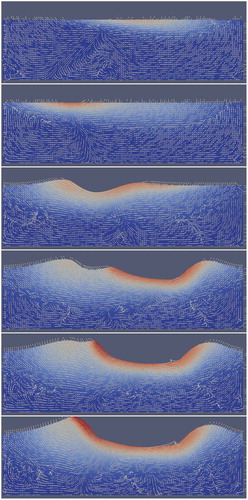
MOOSE 3-D simulation results for the ALE equations are shown in Fig. 1. The simulation was performed with adaptive mesh refinement, with refinement based on gradient jumps in the temperature and z-displacement variables. The number of elements and DOFs changed with refinement, but at the conclusion of the simulation the 3-D domain contained 29 310 elements and 424 018 DOFs. The problem was solved with 12 processes, with approximately 35 000 DOFs per process. The laser is rotated counterclockwise around the top surface of a 3-D cube. When the surface reaches the boiling point of the medium, it recoils, creating an imprint in the surface that tracks with the rotating laser spot. A representative 2-D simulation is shown in Fig. 2, where the laser is swept back and forth repeatedly across the surface. As with the 3-D simulation, melted material is displaced away from the impinging laser spot.

Fig. 1. Visualization of just the top surface of the melt pool after a half and full rotation of the laser. Solid coloring is based on the temperature ranging from 300 K (dark blue) at the bottom of the domain (not shown here) to 3200 K (dark red) at the center of the laser spot. Arrow vectors are based on the velocity vector. Arrow lengths are based on the velocity magnitude and are scaled 10× larger for viewing purposes for the half rotation compared to the full rotation

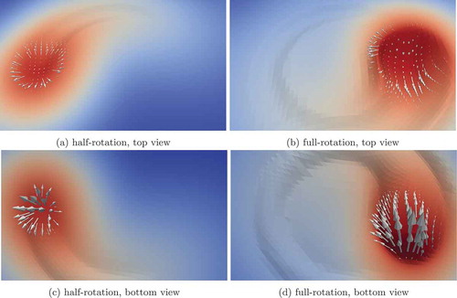
Fig. 2. Two-dimensional melt pool simulation. Arrows represent unscaled velocity vectors. Solid coloring is based on the temperature. Times in arbitrary units are 50, 100, 150, 200, 210, and 220

III.A.2. Multiscale Coupling: Grain Growth in Heat-Affected Zone Near Laser Melt Pool

In processes such as laser welding where a melt pool is formed on the surface of two parts being joined, local changes in the material’s microstructure can result in significant changes in the properties of the material near the weld. As the melt pool resolidifies, the solidification process controls the microstructure and properties of this region. However, the heat input from the laser also causes temperatures to increase significantly outside the melt pool. The region outside the melt pool where temperatures increase enough to cause microstructural changes, but not enough to cause melting, is referred to as the heat-affected zone²² (HAZ).

One of the most significant microstructural changes that can occur in the HAZ is grain growth.²² Grain growth is the process by which the average size of grains increases, driven thermodynamically by the reduction in grain boundary surface area, and therefore, grain boundary energy. Kinetically, grain growth is controlled by the re-arrangement of atoms at grain boundaries and is a strong function of temperature. The average grain size can have a significant impact on mechanical properties. In order to predict the properties, and therefore the performance of a part processed using laser-based techniques such as powder bed fusion or laser welding, it is important to be able to predict microstructural evolution in the HAZ in addition to the resolidifying melt pool. The average grain size in materials is typically much smaller than the size of engineering-scale parts, and it is not computationally practical to perform simulations of microstructural evolution of the entire component. In this section, we employ the multiscale capabilities of the MOOSE framework to address this challenge.

The multiscale coupling strategy employed here uses the ALE-based model of laser melt pool dynamics described in Sec. III.A.1 at the engineering scale, including the temperature field in both the melt pool and the surrounding HAZ. To simulate grain growth in the HAZ, multiple instantiations of the MOOSE phase-field model of grain growth^23,24 are run concurrently with the engineering-scale model using the MOOSE MultiApp system.²⁵ Each instantiation represents microstructural evolution at a different position within the HAZ of the engineering-scale simulation domain. Thus, each grain growth simulation is a representative volume element (RVE) of the macroscale simulation domain. The temperatures at each RVE’s position are passed from the engineering-scale model to the corresponding grain growth simulation using the MOOSE Transfer system.²⁵ A schematic of the coupled simulations is shown in Fig. 3.

Fig. 3. Multiscale demonstration of laser welding with coupled phase-field simulations to determine microstructural evolution in the HAZ. The engineering-scale laser melt pool formation simulation domain is shown in the upper left, with the domain colored by temperature. The simulation domain is 2-D with a size of $0.8\times 0.8$ mm. The laser is incident on the top boundary and travels left to right at a rate of 1 m/min, a typical rate for welding of stainless steel.²⁶ Grain growth simulations are conducted in RVEs at a height of 0.3 and 0.5 mm from the bottom of the engineering-scale simulation domain, as shown with white boxes (boxes are enlarged to ensure visibility). The grain structures at $t=2779$ s are shown in expanded view at the bottom and right. Grain growth simulations are 2-D with a size of 100 $\times$ 100 $\mu$m. Temperatures from the engineering-scale simulations are passed to individual grain growth simulations using the MOOSE Transfer system. The higher temperatures for the grain growth simulations conducted in the RVE at 0.5 mm from the bottom result in a larger grain size, as seen at right

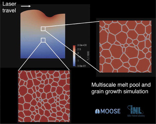
Grain growth simulations were conducted in RVEs as shown in Fig. 3. The RVEs are 2-D with a size of 100 × 100 $\mu$m. The grain structure in the initial conditions is constructed with a Voronoi tessellation as described in Ref. 24, and there are 100 grains in the initial conditions for each simulation. Simplified physical parameters for grain boundary properties were chosen such that a reasonable amount of grain growth occurred in the time span of the weld pool simulation.

The microstructures in both RVEs at the end of the simulation time ($t=2779$ s) are shown in Fig. 3. The average grain size in the RVE at $y=0.5$ mm is larger than that in the RVE at $y=0.3$ mm. The higher temperatures throughout the simulation for the RVE at $y=0.5$ cause the grain boundary mobility to be greater there, resulting in faster grain growth. Further details of the grain growth kinetics will be given in a forthcoming publication.

In this section, we have demonstrated the coupling of an engineering-scale model of laser melt pool formation, enabled by AD, to a phase-field model to quantify the effect of laser heat input on the microstructure in the HAZ. Due to the strong dependence of grain boundary mobility on temperature, relatively small changes in distance from the melt pool result in significantly different grain growth kinetics. This example demonstrates the advantage of leveraging existing multiscale capabilities within the MOOSE framework when using new AD-enabled modeling capabilities.

III.A.3. Melt Pool Level Set

The level-set method is an alternative approach to tracking the free interface in melt pool modeling. In the level-set method, the location of the moving interface is tied to an iso-contour of a scalar field. The mesh is fixed in time and the material moves through the mesh, which makes this technique suitable for severe interface deformations and topology changes. In this work, we use a conservative level-set method^27–30 to accurately model evolution of the liquid-gas interface. The level-set evolution is written as

(2) $\frac{\mathrm{\partial }\varphi }{\mathrm{\partial }t}+\vec{u}(\vec{x},t)\cdot \mathrm{\nabla }\varphi +F_p|\mathrm{\nabla }\varphi |=0,$(2)

where

$\varphi$ =	=	level-set variable
$\vec{u}(\vec{x},t)$ =	=	fluid velocity
$F_p$ =	=	powder addition speed.

For computational efficiency, powder particles are approximately represented as a homogenized continuum medium. The properties are smoothly varied across the interface between gas and solid-liquid using a smeared-out heaviside function defined by the level-set variable.³¹ The density $\rho$, enthalpy $h$, thermal conductivity $k$, and dynamic viscosity $\mu$ in the transition region are provided in Ref. 29. The solid-liquid region of metal is described by pure solid, pure liquid, and solid-liquid mixture (mushy zone) in which the material properties are determined by the mass and volume fraction.

A continuum finite element model is used to describe relevant multiphysics phenomena, including the generation of the powder layer, melting and solidification, melt pool dynamics, and thermal-capillary, buoyant, conductive, and convective heat transport processes. The conservation equations of mass, energy, and momentum are solved with MOOSE.

The gas and liquid flow is assumed to be incompressible, so the mass conservation equation simplifies to

(3) $\mathrm{\nabla }\cdot \vec{u}=0.$(3)

The energy conservation equation is described by

$\begin{array}{rl}& \rho \frac{\mathrm{\partial }h}{\mathrm{\partial }t}+\rho \mathrm{\nabla }\cdot (\vec{u}h)=\mathrm{\nabla }\cdot (k\mathrm{\nabla }T)\\ & +\frac{2P\alpha }{\pi R_b^2}exp\left(\frac{-2r^2}{R_b^2}\right)\left|\mathrm{\nabla }\varphi \right|\\ & -A_h(T-T_0)\left|\mathrm{\nabla }\varphi \right|\\ & -\sigma \in (T^4-T_0^4)\left|\mathrm{\nabla }\varphi \right|\hspace{0.17em}\hspace{0.17em},(4)\end{array}$

where the last three terms on the right represent heat flux from the laser, heat loss through convection, and heat loss through radiation, respectively, and where

$P$ =	=	laser power
$R_b$ =	=	effective beam radius
$\alpha$ =	=	laser energy absorption coefficient
$A_h$ =	=	heat transfer coefficient
$\sigma$ =	=	Stefan-Boltzmann constant
$\in$ =	=	material emissivity
$T_0$ =	=	ambient temperature.

The momentum equation is expressed by

(5) $\rho \left(\frac{\mathrm{\partial }\vec{u}}{\mathrm{\partial }t}+\vec{u}\cdot \mathrm{\nabla }\vec{u}\right)=\mathrm{\nabla }\left[-p\mathbf{I}+\mu \left(\mathrm{\nabla }\vec{u}+\mathrm{\nabla }{\vec{u}}^T\right)\right]-{\rho }_l{\beta }_l\left(T-T_r\right)\vec{g}-\frac{{\mu }_m}{K}\vec{u}+\gamma \vec{n}\kappa |\mathrm{\nabla }\varphi |-{\gamma }_T{\mathrm{\nabla }}_{s}T|\mathrm{\nabla }\varphi |,$(5)

where the last four terms on the right represent buoyancy force, Darcy damping, capillary, and thermal-capillary (Marangoni) forces, respectively, and where

${\beta }_l$ =	=	thermal expansion coefficient
$\vec{g}$ =	=	gravity vector
$T_r$ =	=	reference temperature
$K$ =	=	isotropic permeability
$\gamma$ =	=	surface tension coefficient
$\kappa$ =	=	surface curvature
$\vec{n}$ =	=	normal vector to the free surface
${\gamma }_T$ =	=	thermal-capillary coefficient
${\mathrm{\nabla }}_s$ =	=	surface gradient operator.

Equations (2)(2) $\frac{\mathrm{\partial }\varphi }{\mathrm{\partial }t}+\vec{u}(\vec{x},t)\cdot \mathrm{\nabla }\varphi +F_p|\mathrm{\nabla }\varphi |=0,$(2) through (5(5) $\rho \left(\frac{\mathrm{\partial }\vec{u}}{\mathrm{\partial }t}+\vec{u}\cdot \mathrm{\nabla }\vec{u}\right)=\mathrm{\nabla }\left[-p\mathbf{I}+\mu \left(\mathrm{\nabla }\vec{u}+\mathrm{\nabla }{\vec{u}}^T\right)\right]-{\rho }_l{\beta }_l\left(T-T_r\right)\vec{g}-\frac{{\mu }_m}{K}\vec{u}+\gamma \vec{n}\kappa |\mathrm{\nabla }\varphi |-{\gamma }_T{\mathrm{\nabla }}_{s}T|\mathrm{\nabla }\varphi |,$(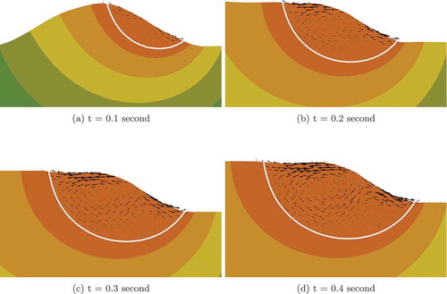5) ) are solved implicitly in MOOSE. These equations are highly nonlinear and strongly coupled, so accurate Jacobians are required for Newton’s method to converge appropriately. With AD, we are able to form perfect Jacobians and solve the equations in a fully coupled manner. In the example considered, only three to four nonlinear iterations are needed to solve each time step, making the overall simulation remarkably efficient. The material considered here is 316L stainless steel; parameters relevant to the simulation can be found in Refs. 27 through 30. The initial and melting temperatures are set to be 300 and 1673 K, respectively. The predicted sequential track evolution during 0.4 s of the process is illustrated in Fig. 4. The melt pool is generated at the front of the track corresponding to the laser spot. Due to the high cooling rate, the melt solidifies shortly after the laser moves away. The fluid motion in the melt pool is shown in Fig. 5. The liquid flows from the higher-temperature region toward the lower-temperature region due to thermal-capillary forces. The fluid velocity is damped outside the fluid domain due to the Darcy effect. Two vortices form in the melt pool by t = 0.2 s; the vortex pattern is consistent with simulation results shown in Refs. 27 and 29. Although only 2-D results are shown here, the model and implementation can be readily applied to three dimensions.

Fig. 4. Sequential deposition profile and temperature distribution. The coloring is based on the temperature ranging from 300 to 1782 K

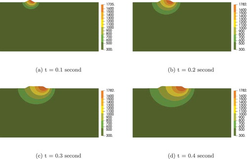
Fig. 5. Sequential fluid motion velocity fields in the melt pool. Arrows represent scaled velocity vectors. The scale of the temperature is shown in Fig. 4. The white line shows the contour of the melting temperature

III.B. Neural Network–Based Free Energies in Phase-Field Modeling

In the field of mesoscale materials modeling, the phase-field method has emerged as a well-established approach for simulating the co-evolution of microstructure and proper-ties.^32,33 The description of phase-state and concentrations through field variables with finite-width smooth interfaces has proven to be an extremely flexible approach resulting in a broad range of applications from solidification^34,35 to over-phase transformation^36,37 to grain growth.^23,38

Quantitative phase-field modeling of realistic material systems requires thermodynamic and kinetic input data in the form of Gibbs free energies and atomic mobilities. The assessment and compilation of such data through a combination of theoretical and experimental data are formalized by the CALPHAD approach.³⁹ In CALPHAD, Gibbs free energies are expressed as phenomenological function expansions combined with semi-empirical entropy models. As a standard machine readable delivery format for these free energies, the thermodynamic database ASCII-based file format has been established, and a large swath of open thermodynamic and kinetic data exists on the web and can be explored with search engines such as the Thermodynamic DataBase DataBase.⁴⁰

CALPHAD free-energy databases present users with two challenges. Commercial databases are often encrypted and do not permit the extraction of functional forms and parameter sets. Free-energy formulations in the compound energy formalism allow for phases with multiple sublattices. The distribution of the local solute concentrations onto the different sublattices requires solving a local free-energy minimization problem, which comes at a computational cost. Both issues can be addressed by pretabulating the free-energy functions over the configuration space relevant to the phase-field problem at hand and generating a surrogate model for the tabulated free energy to ensure differentiability and smoothness.

In this work, we propose the use of multilayer neural networks as a generic function fitting tool to generate surrogate free-energy models from pretabulated free-energy data, which can be obtained from thermodynamic database software, such as ThermoCalc or pycalphad. We rely on the universal function approximation theorem,⁴¹ which states that any continuous function over the ${\mathbb{R}}^n$ can be approximated with an arbitrarily small error using a neural network with one hidden layer and a finite number of neurons.

We chose a fully connected network topology with a variable number of hidden layers and hidden layer nodes. The input nodes of the network are connected to the state space coordinates $\vec{s}$ or arguments of the free-energy function, such as temperature, concentrations, pressure, etc. The output node is the value of the free energy. We note that while the implementation of training and evaluation of the neural network allows for an arbitrary number of input and output nodes, in the context of this work we use a single output node for the value of the free energy.

The chemical potential data are not fitted independently from the free-energy data, as the chemical potentials are the derivatives of the free energy with respect to its arguments, or in terms of a neural network, the derivatives of the output node with respect to the input nodes. We have derived an analytical expression for these derivatives. Not having independent training for the chemical potentials ensures the free energy and chemical potentials remain consistent and that a closed loop in state space does not incur a difference in free energy.

A multilayer perceptron network with two hidden layers can be described by

(6) $F(\vec{s})={\left[{\left[\vec{s}\cdot W_1+{\vec{b}}_1\right]}_g\cdot W_2+{\vec{b}}_2\right]}_g\cdot W_3+{\vec{b}}_3,$(6)

where

$W_i$ = $n_i\times n_{i-1}$ weight matrices that code the connectivity between the adjacent layers containing $n_i$ and $n_{i-1}$ neurons, respectively

${\vec{b}}_i$ = a bias vector

$[\dots {]}_g$ = elementwise application of the activation function (a sigmoid or softsign).

Training of the networks has been implemented using the PyTorch machine learning framework,⁴² which supports GPU-accelerated learning. The networks are trained outside of MOOSE in a standalone PyTorch-based python code. Once trained, the network topology and parameterization contained in the $W_i$ matrices and ${\vec{b}}_i$ vectors are exported to a simple text file format. We read these files in the MOOSE-based Marmot application for mesoscale microstructure modeling. Evaluation of the networks and the first derivative of the output node(s) with respect to the input nodes are performed in Marmot.

We utilize dual numbers and forward-mode AD to obtain the second derivatives of the output node (i.e., the first derivative of the chemical potentials with respect to the DOFs of the state-space variables we are solving for). The derivative $\frac{\mathrm{\partial }F}{\mathrm{\partial }\vec{s}}$ is straightforward to derive analytically. This permits us to construct the exact Jacobian matrix for the Cahn-Hilliard phase-field problem.

To test the feasibility of a neural network–based free-energy density, we trained a network on an analytical free-energy density function. This approach allows us to compare the neural network results to the exact solution. We generated an evenly sampled set of data points of the regular solution free-energy density function

(7) $F(c,T)=\omega c_p(1-c_p)+\chi T{\left(c_{p}log(c_p)+(1-c_p)log(1-c_p)\right)}^2,$(7)

with $\omega =1$ and $\chi ={10}^{-3}$ at intervals $\mathrm{\Delta }c={10}^{-3}$ in the interval $[0.05,0.95]$, and $\mathrm{\Delta }T=6\mathrm{K}$ in the interval $[445\mathrm{K},475\mathrm{K}]$. The loss function $L$ is computed using the values of the free-energy training values ${\bar{F}}_n$ and the network’s predicted value $F_n$, as well as their derivatives with respect to the input node values $\vec{s}=(c,T)$ as

(8) $L=\frac{1}{N}\sum _n^N{\left({\bar{F}}_n-F_n\right)}^2+\left(\frac{\mathrm{\partial }{\bar{F}}_n}{\mathrm{\partial }\vec{s}}-\frac{\mathrm{\partial }{F}_n}{\mathrm{\partial }\vec{s}}\right).$(8)

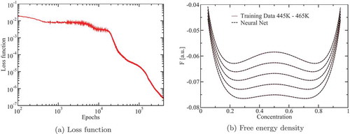
Training was stopped at 400 000 epochs and a wall time of about 1 h on a GeForce RTX 2080 (Fig. 6a). A comparison of the free energies returned by the neural network and the training data is shown in Fig. 6b. As expected from the loss function value, the curves are visually indistinguishable.

Fig. 6. Loss function and free-energy density

Next, we implemented the evaluation of the neural network in Marmot. Here the forward-mode AD simplified the implementation effort greatly by providing us with the derivatives of the chemical potentials with respect to the finite element DOFs.

To test the neural network free energy, we set up two concentration fields $c_p$ and $c_n$. Both fields were initialized with identical fields generated from a uniform random distribution of values between 0.45 and 0.55, right in the middle of the spinodal region of the phase diagram for the free-energy density function $F(c,T)$. We evolved both fields using the time-dependent Cahn-Hilliard equation, choosing the analytical free-energy expression from Eq. (7)(7) $F(c,T)=\omega c_p(1-c_p)+\chi T{\left(c_{p}log(c_p)+(1-c_p)log(1-c_p)\right)}^2,$(7) for the $c_p$ field and the neural network free energy for the $c_n$ field. The simulations were run with $T=460$ K for 750 time units.

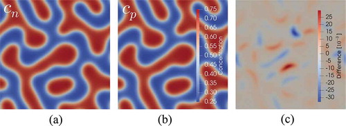
The results of the simulation are shown in Fig. 7. The time-integrated concentration fields are qualitatively very similar. Only differencing the fields, as shown in Fig. 7a, reveals a subtle difference on the order of 1% in concentration. This is an indication of how sensitive the microstructural evolution is to even small changes in the free-energy density function.

Fig. 7. Cahn-Hilliard spinodal decomposition phase-field simulation showing the concentration field $c_n$ for (a) neural network–based free energy, (b) the concentration field $c_p$ for the corresponding analytical free energy, which the neural network was trained on, and (c) the difference between the two fields

In summary, we believe using neural network–based surrogate models for thermodynamic potentials is a viable approach that needs to be investigated further. Automatic differentiation in MOOSE significantly accelerated the implementation of a neural network in our mesoscale microstructure evolution code.

III.C. Nuclear Fuel Performance Simulations

Fuel performance simulation is a powerful tool utilized to try and predict the behavior of actinide fuel and steel cladding in the high-temperature irradiation conditions experienced in nuclear reactor cores.⁴³ Such simulations are made difficult not only by the complex operating environment, but also by the inability to obtain the high volume of data required to build comprehensive empirical constitutive models that can be used to describe the thermomechanical response of the fuel and cladding beyond typical operating conditions. Consequently, the need for predictive rather than descriptive tools to fill in the holes between sparse data sets requires mechanistic models that stretch both academic understanding and computational limits.

Like all nuclear fuel, metallic fuel (here, metallic will only refer to zirconium-based metallic fuel, e.g., U-Zr and U-Pu-Zr) suffers from volumetric swelling during irradiation due to the accumulation of fission gas into bubbles. Once the bubbles interconnect with an outside surface, the fission gas is released into the fuel plenum, imparting a pressure loading on the thin cladding. Over time, the internal pressure in the fuel pin plenum will result in thermal and irradiation creep of the cladding. If enough deformation occurs, the swelled fuel pin can place the core at risk of overheating due to coolant channel restriction, further enhancing plastic deformation. If left unchecked, the cladding could fail, releasing radioactive gases into the coolant. Using this simplified description of nuclear fuel pin behavior during irradiation, two driving factors can be identified as key components in understanding cladding failure: fission gas swelling in the fuel and creep behavior in the cladding.

While lower-length-scale atomistic and microstructural simulations of nuclear fuel utilize a wide range of computational methods such as density functional theory, molecular dynamics, and Monte Carlo, fuel performance simulations almost always rely on a finite element framework to capture the thermomechanical response of fuel systems.⁴⁴ Such highly coupled nonlinear problems often have been explored with the MOOSE framework, primarily through the BISON code.⁴³ Although the historical focus of BISON has been primarily on the UO₂/Zircaloy system due to familiarity of the fuel system in the United States, recent progress at modeling zirconium-based metallic fuel has accelerated due to the AD methods described here.⁴⁵ Several examples of advanced mechanistic models will be summarized in order to provide a sense of how AD has enabled rapid implementation of advanced mechanistic constitutive models into BISON.

III.C.1. The Tangent Modulus

The strain in a material $\epsilon$ can be decomposed into several components:

(9) $\epsilon ={\epsilon }^{el}+{\epsilon }^{th}+{\epsilon }^{sw}(\sigma )+{\epsilon }^{cr}(\sigma ),$(9)

where

${\epsilon }^{el}$ =	=	elastic strain
${\epsilon }^{th}$ =	=	thermal strain
${\epsilon }^{sw}$ =	=	swelling strain (e.g., fission gas or void swelling)
${\epsilon }^{cr}$ =	=	creep strain.

The typical constitutive equation used to compute the stress $\sigma$ to the elastic strain, is

(10) $\sigma =\mathbb{C}:{\epsilon }^{el}=\mathbb{C}:\left[\epsilon -{\epsilon }^{sw}(\sigma ){\epsilon }^{th}-{\epsilon }^{cr}(\sigma )\right],$(10)

where $\mathbb{C}$ is the elasticity tensor. Since the swelling and creep strains can be dependent on the stress, Eq. (10)(10) $\sigma =\mathbb{C}:{\epsilon }^{el}=\mathbb{C}:\left[\epsilon -{\epsilon }^{sw}(\sigma ){\epsilon }^{th}-{\epsilon }^{cr}(\sigma )\right],$(10) becomes a complex set of nonlinear partial differential equations that is typically solved using inner Newton-Raphson root-finding loops such as radial return algorithms.⁴⁶ This in turn requires a proper Jacobian once converged, which is typically in the form of the so-called tangent modulus $\mathbb{J}$:

(11) $d{\sigma }_{n+1}=\mathbb{J}:d{\epsilon }_{n+1},$(11)

where $\mathbb{J}$ represents the change in stress as a function of strain and typically describes the stiffness of a material in the plastic range. In the limit where a material response is primarily elastic $\mathbb{J}\simeq \mathbb{C}$. However, due to the nonlinearity introduced by stress-dependent strain, $\mathbb{J}$ quickly becomes a nontrivial derivation with potentially no closed form. Like the other Jacobians described here, Eq. (10)(10) $\sigma =\mathbb{C}:{\epsilon }^{el}=\mathbb{C}:\left[\epsilon -{\epsilon }^{sw}(\sigma ){\epsilon }^{th}-{\epsilon }^{cr}(\sigma )\right],$(10) can be solved without a perfectly defined $\mathbb{J}$, either through brute force computation using perturbation techniques, small time steps, or finite differencing.⁴⁷ Unfortunately, these simplifications tend to result in unacceptable increases in computational cost or time to justify their implementation in fuel performance simulations. Even formulation of an analytical $\mathbb{J}$ leads to extensive mathematic manipulation that quickly overshadows the implementation of any mechanistic modeling.

With the introduction of AD into MOOSE, the formulation of $\mathbb{J}$ is handled automatically, even allowing for Jacobian information to propagate through to the outer Newton-Raphson algorithm. This has allowed rapid prototyping of advanced constitutive models for the fuel and cladding, both of which are descried briefly here and will be explored in detail in future publications. The goal of the following examples is to convey how the use of AD in MOOSE has allowed for implementation and testing of advanced mechanistic models before fully committing to a comprehensive derivation by forgoing the need to formulate an accurate $\mathbb{J}$.

III.C.2. Fission Gas Swelling

While the driving mechanism for the growth of fission gas bubbles is simple (i.e., accumulation of fission gas), the volumetric strain response is nontrivial. In general, the bubble surface can be assumed to be in equilibrium with the surrounding material due to the fast mobility and high concentration of vacancies present in the fuel during irradiation.⁴⁸ As a first approximation, the bubble radius $r$ can be estimated via the Young-Laplace equation with a van der Waals equation of state by equating the pressure of the gas $P_{gas}$ to the pressure exerted by the surface $P_{surf}$ (Ref. 45):

(12) $P_{gas}=P_{surf}$(12)

and

(13) $\frac{k_{B}T}{v_b(r)/g_b(r)-B}=2{\gamma }_s/r-{\sigma }_{hydro}(r),$(13)

where

$k_B$ =	=	Boltzmann constant
$T$ =	=	temperature
$v_b$ =	=	volume of the bubble
$B$ =	=	van der Waals constant for the gas
${\gamma }_s$ =	=	surface tension
${\sigma }_{hydro}$ =	=	bulk stress at the surface of the bubble.

By turning Eq. (13)(13) $\frac{k_{B}T}{v_b(r)/g_b(r)-B}=2{\gamma }_s/r-{\sigma }_{hydro}(r),$(13) into a residual, an inner Newton loop can be utilized to solve for the bubble radius $r$. This in turn can be used to apply a volumetric strain on the cladding:

(14) $\frac{\mathrm{\Delta }V}{V}=\frac{4}{3}\pi r^3{C}_b,$(14)

where $C_b$ is the concentration of bubbles in the solid. Despite the many built-in simplifications, Eq. (13)(13) $\frac{k_{B}T}{v_b(r)/g_b(r)-B}=2{\gamma }_s/r-{\sigma }_{hydro}(r),$(13) turns into a seven-order polynomial due to the stress coupling term in $\sigma$. Furthermore, the growth of the porosity in the fuel $f$ can be calculated from the individual swelling strain components:

(15) $\dot{f}=[1.0-f]\ast \left({\dot{\in }}_{xx}^{sw}+{\dot{\in }}_{yy}^{sw}+{\dot{\in }}_{zz}^{sw}\right)\hspace{0.17em}\hspace{0.17em}.$(15)

The growing porosity will impact the strength of the fuel via the elasticity tensor $\mathbb{C}$ and the temperature of the fuel via the thermal conductivity, convoluting the solution of Eq. (10)(10) $\sigma =\mathbb{C}:{\epsilon }^{el}=\mathbb{C}:\left[\epsilon -{\epsilon }^{sw}(\sigma ){\epsilon }^{th}-{\epsilon }^{cr}(\sigma )\right],$(10) even further.

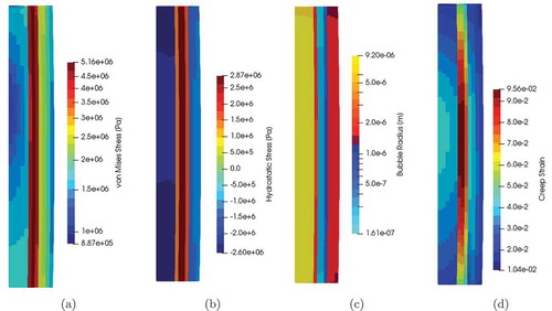
The ability to quickly implement a complex model like Eq. (13)(13) $\frac{k_{B}T}{v_b(r)/g_b(r)-B}=2{\gamma }_s/r-{\sigma }_{hydro}(r),$(13) using AD has allowed for rapid prototyping and model refinement. More importantly, advanced models allow for quantification of potential approximations rather than being forced to make decisions a priori. Following the results from the example simulations (Fig. 8), the rapid prototyping has led to increased interest and funding in refining and calibrating this bubble model.

Fig. 8. Results from simulation of a prototypical U-Pu-Zr rodlet fuel performance simulation at an intermediate time in order to illustrate the impact of the bubble model on the (a) von Mises stress, (b) hydrostatic stress, (c) radius, and (d) creep strain.⁴⁵ Note, cladding is omitted for clarity. The radial variation is due to phase-dependent bubble concentrations and sizes

III.C.3. Reduced-Order Model for Cladding Creep

With cladding strain as one of the primary concerns for core integrity, accurate estimations of the creep response to internal plenum pressure is essential to help reduce costly overestimations resulting in unnecessarily large failure margins or dangerous underestimations that could allow for dangerous core failures. In order to maximize the utilization of irradiated steel experimental campaigns, mechanistic modeling must be used to bridge the sparsity of data.

Recently, a mechanistic-based constitutive creep model for HT9 stainless steels was developed through extensive simulations using the visco-plastic self-consistent (VPSC) approach.^49,50 This provided a tool to estimate creep response for standard fast reactor cladding in a predictive manner. Unfortunately, this lower-length (i.e., microstructural) code is too vastly expensive to run concurrently within a fuel performance simulation. In addition, the creep strain response in HT9 is dependent on several evolving parameters, such as dislocation density, preventing an analytical creep rate formulation.

In order to overcome the computational cost of the VPSC simulations while still enabling a mechanistic, lower-length-scale-informed constitutive HT9 model, a reduced-order method (ROM) to condense hundreds of precomputed VPSC results into orthogonal Legendre polynomials has shown promise in similar stainless steels.⁵¹ These polynomials carry the form

(16) ${\epsilon }^{cr}(\sigma )=\sum _{w=0}^{deg}\dots \sum _{z=0}^{deg}{\alpha }_{w\dots z}{P}_w\left(x_w\right)\dots P_z\left(x_z\right),$(16)

where

$P_i\left(x\right)$ = polynomial of degree $i$

$deg$ = maximum degree of polynomial to be used in the model (typically two or three)

${\alpha }_i$ regression coefficients for the terms formed from the product of the i’th degree polynomial of input $x_i$.

By calibrating the various Legendre coefficients to the VPSC data, Eq. (16)(16) ${\epsilon }^{cr}(\sigma )=\sum _{w=0}^{deg}\dots \sum _{z=0}^{deg}{\alpha }_{w\dots z}{P}_w\left(x_w\right)\dots P_z\left(x_z\right),$(16) can be trained to provide a nearly identical creep strain response with a fraction of the computational cost.

Although an analytical expression for the tangent modulus that derives from Eq. (16)(16) ${\epsilon }^{cr}(\sigma )=\sum _{w=0}^{deg}\dots \sum _{z=0}^{deg}{\alpha }_{w\dots z}{P}_w\left(x_w\right)\dots P_z\left(x_z\right),$(16) may be possible, the rapid implementation in MOOSE using AD allowed for early prototyping to support adoption of an HT9 ROM using a limited number of VPSC simulations to formulate the Legendre polynomial coefficients. Similar to the fission gas swelling model, increased resources were consequently diverted to develop a fully calibrated ROM for use in metallic fuel performance simulations.

IV. CONCLUSIONS AND FUTURE WORK

The introduction of MetaPhysicL and AD into the MOOSE framework has opened doors to simulation types that were not previously possible because of the complexity of forming accurate hand-coded Jacobians or because the multiphysics nature of the problem inhibited the accuracy of finite difference approximations. Examples of these simulations include ALE and level-set models of laser melt pools, phase-field models with neural network–based free energies, and metallic nuclear fuel performance calculations that rely on extensive inner Newton loops for material property evaluation. Future AD work includes the exploration of dynamic derivative storage containers using a memory pool in order to reduce the memory footprint for dynamic mesh calculations that require storing derivative information with respect to displacements for each mesh node. If the memory pool implementation is successful, it will allow expansion of AD into more complex discretization schemes such as mortar methods for nonconforming interfaces.

Acronyms

2-D:   two dimensional

3-D:   three dimensional

AD:   automatic differentiation

ALE:   arbitrary Lagrangian-Eulerian

DOE:  U.S. Department of Energy

DOF:  degree of freedom

GMRES: generalized minimal residual method

HAZ:  heat affected zone

JFNK:  Jacobian-Free Newton-Krylov

MASA: Manufactured Analytical Solution Abstraction library

MOOSE: Multiphysics Object Oriented Simulation Environment

PJFNK: preconditioned Jacobian-Free Newton-Krylov

SLM:  selective laser melting

ROM:  reduced-order method

RVE:  representative volume element

VPSC:  visco-plastic self-consistent

Acknowledgments

This work was sponsored in part by the U.S. Department of Energy (DOE), Office of Nuclear Energy, Nuclear Energy Advanced Modeling and Simulation program and Idaho National Laboratory’s Laboratory Directed Research & Development Program. Idaho National Laboratory, an affirmative action/equal opportunity employer, is operated by Battelle Energy Alliance under contract number DE-AC07-05ID14517. Los Alamos National Laboratory, an affirmative action/equal opportunity employer, is operated by Triad National Security, LLC, for the National Nuclear Security Administration of the DOE under contract number 89233218CNA000001.

References

- C. J. PERMANN et al., “MOOSE: Enabling Massively Parallel Multiphysics Simulation,” SoftwareX, 11, 100430 (2020); https://doi.org/10.1016/j.softx.2020.100430.
- J. BROWN, “Why Is Newton’s Method Not Converging?”; https://scicomp.stackexchange.com/q/30/24756 ( current as of June 17, 2020).
- D. A. KNOLL and D. E. KEYES, “Jacobian-Free Newton–Krylov Methods: A Survey of Approaches and Applications,” J. Comput. Phys., 193, 2, 357 (2004); https://doi.org/10.1016/j.jcp.2003.08.010.
- A. MEURER et al., “SymPy: Symbolic Computing in Python,” PeerJ Comput. Sci., 3, e103 (2017); https://doi.org/10.7717/peerj-cs.103.
- S. WOLFRAM et al., The MATHEMATICA® Book, Version 4, Cambridge University Press (1999).
- A. GRIEWANK et al., “On Automatic Differentiation,” Math. Program. Recent Dev. Appl., 6, 6, 83 (1989).
- A. PASZKE et al., Automatic Differentiation in Pytorch (2017); https://openreview.net/pdf?id=BJJsrmfCZ.
- J. I. TOIVANEN and R. A. MÄKINEN, “Implementation of Sparse Forward Mode Automatic Differentiation with Application to Electromagnetic Shape Optimization,” Optim. Methods Software, 26, 4–5, 601 (2011); https://doi.org/10.1080/10556781003642305.
- N. MALAYA et al., “MASA: A Library for Verification Using Manufactured and Analytical Solutions,” Eng. Comput., 29, 4, 487 (2013); https://doi.org/10.1007/s00366-012-0267-9.
- C. CARTIS and L. ROBERTS, “A Derivative-Free Gauss-Newton Method,” Math. Program. Comput., 11, 4, 631 (2019); https://doi.org/10.1007/s12532-019-00161-7.
- S. BALAY et al., “PETSc Users Manual,” ANL-95/11-Revision 3.13, Argonne National Laboratory (2020); https://www.mcs.anl.gov/petsc(current as of June 17, 2020).
- K. V. WONG and A. HERNANDEZ, “A Review of Additive Manufacturing,” Int. Scholarly Res. Notices, 2012, 208760 (2012); https://doi.org/10.5402/2012/208760.
- A. HUSSEIN et al., “Finite Element Simulation of the Temperature and Stress Fields in Single Layers Built Without-Support in Selective Laser Melting,” Mater. Des. (1980–2015), 52, 638 (2013); https://doi.org/10.1016/j.matdes.2013.05.070.
- L. PARRY, I. ASHCROFT, and R. D. WILDMAN, “Understanding the Effect of Laser Scan Strategy on Residual Stress in Selective Laser Melting Through Thermo-Mechanical Simulation,” Addit. Manuf., 12, 1 (2016); https://doi.org/10.1016/j.addma.2016.05.014.
- “ANSYS,” ANSYS; https://www.ansys.com ( current as of June 17, 2020).
- “MSC Marc,” M. SOFTWARE; https://www.mscsoftware.com/product/marc ( current as of June 17, 2020).
- S. A. KHAIRALLAH and A. ANDERSON, “Mesoscopic Simulation Model of Selective Laser Melting of Stainless Steel Powder,” J. Mater. Process. Technol., 214, 11, 2627 (2014); https://doi.org/10.1016/j.jmatprotec.2014.06.001.
- C. R. NOBLE et al., “ALE3D: An arbitrary Lagrangian-Eulerian Multi-Physics Code,” Lawrence Livermore National Laboratory (2017).
- D. R. NOBLE et al., “Use of Aria to Simulate Laser Weld Pool Dynamics for Neutron Generator Production,” Sandia National Laboratories (2007).
- H. LI et al., “3D Numerical Simulation of Successive Deposition of Uniform Molten Al Droplets on a Moving Substrate and Experimental Validation,” Comput. Mater. Sci, 65, 291 (2012); https://doi.org/10.1016/j.commatsci.2012.07.034.
- M. S. BENI, T. H. TAN, and K. YU, “Atomistic Modeling of Pileup Process in Metal Deposition Manufacture,” Results Phys., 12, 1660 (2019); https://doi.org/10.1016/j.rinp.2019.01.075.
- D. PORTER and K. EASTERLING, Phase Transformations in Metals and Alloys, Chapman and Hall, London (1992).
- N. MOELANS, B. BLANPAIN, and P. WOLLANTS, “Quantitative Analysis of Grain Boundary Properties in a Generalized Phase Field Model for Grain Growth in Anisotropic Systems,” Phys. Rev. B, 78, 2, 024113 (23 pages) (2008); https://doi.org/10.1103/PhysRevB.78.024113.
- C. J. PERMANN et al., “Order Parameter Remapping Algorithm for 3D Phase Field Model of Grain Growth Using FEM,” Comput. Mater. Sci, 115, 18 (2016); https://doi.org/10.1016/j.commatsci.2015.12.042.
- C. J. PERMANN et al., “MOOSE: Enabling Massively Parallel Multiphysics Simulation,” SoftwareX, 11, 100430 (2020); https://doi.org/10.1016/j.softx.2020.100430, ArXiv e-print: https://arxiv.org/abs/1911.04488 (current as of June 17, 2020).
- J. D. MADISON and L. K. AAGESEN, “Quantitative Characterization of Porosity in Laser Welds of Stainless Steel,” Scr. Mater., 67, 9, 783 (2012); https://doi.org/10.1016/j.scriptamat.2012.06.015.
- H.-O. ZHANG et al., “Numerical Simulation of Multiphase Transient Field During Plasma Deposition Manufacturing,” J. Appl. Phys., 100, 12, 123522 (2006); https://doi.org/10.1063/1.2399341.
- X. HE and J. MAZUMDER, “Transport Phenomena During Direct Metal Deposition,” J. Appl. Phys., 101, 5, 053113 (2007); https://doi.org/10.1063/1.2710780.
- S. WEN and Y. C. SHIN, “Modeling of Transport Phenomena During the Coaxial Laser Direct Deposition Process,” J. Appl. Phys., 108, 4, 044908 (2010); https://doi.org/10.1063/1.3474655.
- M. COURTOIS et al., “A Complete Model of Keyhole and Melt Pool Dynamics to Analyze Instabilities and Collapse During Laser Welding,” J. Laser Appl., 26, 4, 042001 (2014); https://doi.org/10.2351/1.4886835.
- E. OLSSON and G. KREISS, “A Conservative Level Set Method for Two Phase Flow,” J. Comput. Phys., 210, 1, 225 (2005); https://doi.org/10.1016/j.jcp.2005.04.007.
- L.-Q. CHEN, “Phase-Field Models for Microstructure Evolution,” Annu. Rev. Mater. Res., 32, 1, 113 (2002); https://doi.org/10.1146/annurev.matsci.32.112001.132041.
- N. MOELANS, B. BLANPAIN, and P. WOLLANTS, “An Introduction to Phase-Field Modeling of Microstructure Evolution,” CALPHAD, 32, 2, 268 (2008); https://doi.org/10.1016/j.calphad.2007.11.003.
- J. A. WARREN and W. J. BOETTINGER, “Prediction of Dendritic Growth and Microsegregation Patterns in a Binary Alloy Using the Phase-Field Method,” Acta Metall. Mater., 43, 2, 689 (1995); https://doi.org/10.1016/0956-7151(94)00285-P.
- A. KARMA and W.-J. RAPPEL, “Phase-Field Method for Computationally Efficient Modeling of Solidification with Arbitrary Interface Kinetics,” Phys. Rev. E, 53, 4, R3017 (4 pages) (1996); https://doi.org/10.1103/PhysRevE.53.R3017.
- A. A. WHEELER, W. J. BOETTINGER, and G. B. McFADDEN, “Phase-Field Model for Isothermal Phase Transitions in Binary Alloys,” Phys. Rev. A., 45, 10, 7424 (1992); https://doi.org/10.1103/Phys-RevA.45.7424.
- S. G. KIM, W. T. KIM, and T. SUZUKI, “Phase-Field Model for Binary Alloys,” Phys. Rev. E, 60, 6, 7186 (1999); https://doi.org/10.1103/PhysRevE.60.7186.
- D. FAN and L.-Q. CHEN, “Diffusion-Controlled Grain Growth in Two-Phase Solids,” Acta Mater., 45, 8, 3297 (1997); https://doi.org/10.1016/S1359-6454(97)00022-0.
- H. L. LUKAS et al., Computational Thermodynamics: The Calphad Method, Vol. 131, Cambridge University Press, Cambridge (2007).
- A. VAN DE WALLE, C. NATARAJ, and Z.-K. LIU, “The Thermodynamic Database Database,” Calphad, 61, 173 (2018); https://doi.org/10.1016/j.calphad.2018.04.003.
- M. LESHNO et al., “Multilayer Feedforward Networks with a Nonpolynomial Activation Function Can Approximate Any Function,” Neural Networks, 6, 6, 861 (1993); https://doi.org/10.1016/S0893-6080(05)80131-5.
- A. PASZKE et al. “PyTorch: An Imperative Style, High-Performance Deep Learning Library,” H. WALLACH et al., Eds., Advances in Neural Information Processing Systems 3 2, pp. 8024–8035, Curran Associates, Inc. (2019); http://papers.neurips.cc/paper/9015-pytorch-an-imperative-style-high-performance-deep-learning-library.pdf (current as of June 17, 2020).
- R. L. WILLIAMSON et al., “Multidimensional Multiphysics Simulation of Nuclear Fuel Behavior,” J. Nucl. Mater., 423, 1–3, 149 (2012); https://doi.org/10.1016/j.jnucmat.2012.01.012.
- M. R. TONKS et al., “Mechanistic Materials Modeling for Nuclear Fuel Performance,” Ann. Nucl. Energy, 105, 11 (2017); https://doi.org/10.1016/j.anucene.2017.03.005.
- C. MATTHEWS et al., “Improvements to the Multi-Scale Capabilities of BISON for Metallic Fuel Performance Modeling,” LA-UR-19-29858, Los Alamos National Laboratory (2019).
- J. C. SIMO and R. L. TAYLOR, “Consistent Tangent Operators for Rate-Independent Elasto-Plasticity,” Comput. Methods Appl. Mech. Eng., 48, 1, 101 (1985); https://doi.org/10.1016/0045-7825(85)90070-2.
- N. PRAKASH et al., “A General Constitutive Framework for the Combined Creep, Plasticity and Swelling Behavior of Nuclear Fuels in an Implicit Hypoelastic Formulation,” Los Alamos National Laboratory (2019).
- D. R. OLANDER, “Fundamental Aspects of Nuclear Reactor Fuel Elements,” Technical Information Center, U.S. Department of Energy (1976).
- W. WEN et al., “Mechanism-Based Modeling of Thermal and Irradiation Creep Behavior: An Application to Ferritic/Martensitic HT9 Steel,” Int. J. Plast., 126, 102633 (2020); https://doi.org/10.1016/j.ijplas.2019.11.012.
- R. A. LEBENSOHN and C. N. TOMÉ, “A Self-Consistent Anisotropic Approach for the Simulation of Plastic Deformation and Texture Development of Polycrystals: Application to Zirconium Alloys,” Acta Metall. Mater., 41, 9, 2611 (1993); https://doi.org/10.1016/0956-7151(93)90130-K.
- A. E. TALLMAN et al., “Data-Driven Constitutive Model for the Inelastic Response of Metals: Application to 316H Steel,” Integr. Mater. Manuf. Innovation, 9, 339 (2020); https://doi.org/10.1007/s40192-020-00181-5.