Location and Activity Characterization of Gamma-Ray Point Sources Concealed in Shipping Containers Using Iterative Reconstruction and Modeling Cargo-Specific Attenuation

Abstract

Simulated measurements of traditional shipping container screening infrastructure based on large-area polyvinyl-toluene (PVT) or sodium-iodide detectors (NaI) are used alongside an iterative reconstruction algorithm to characterize the activity and location of a radioactive point source concealed within a shipping container loaded with cargo. A maximum likelihood expectation maximization reconstruction method is employed to reconstruct the source distribution under the assumption that there exists a single point source in the scenario.

To account for shielding by the cargo, it is assumed that the encompassing cargo, which was chosen to represent iron cargo, such as scrap metal or machine parts, is homogeneously distributed throughout the 32.2-m³ container at realistic loaded container densities of 0.0, 0.2, or 0.6 gcm⁻³. When the material properties of the cargo are assumed known and provided to the algorithm, the method is capable of localizing the source to within 40.5 cm and estimating the activity to the correct order of magnitude for cases with no cargo and 0.2 gcm⁻³ iron cargo completely filling the 32.2-m³ volume. With iron cargo at a density of 0.6 gcm⁻³, the localization and activity estimation is significantly worse, which is attributed to the method of accounting for attenuation in the cargo, a decreased signal-to-noise ratio, and the use of gross-count data that include the effect of buildup radiation. Using 662-keV photopeak data from a NaI-based radiation portal monitor (RPM) achieves better results than gross-count data from a PVT- or NaI-based RPM with the correct order of magnitude activity estimates for all cargo densities.

For scenarios where the material of the cargo is unknown, but its density and distribution are known, a brute-force search is performed to find the optimum mass attenuation coefficient that describes the cargo. From the range of mass attenuation coefficients obtained, the method is not capable of differentiating between different types of common cargo, but demonstrates the principle of the method for characterizing shipping container cargo. Ultimately, the largest limiting factor in this method is the use of a simple average to estimate the path length traveled from a point in the container through the cargo in the direction of a detector. The large area detectors result in a high variance in this path length, and the degree of attenuation is exponentially dependent on this value.

Despite the simple method of accounting for attenuation in the cargo, the maximum likelihood expectation maximization point source (MLEM PS) method is able to characterize a concealed point source well in the case with a PVT-based RPM and 0.2 gcm⁻³, which is cargo above the average density of a shipping container, drastically reducing the search area in secondary screening processes. The MLEM PS algorithm, therefore, represents a means of enhancing shipping container screening procedures without requiring significant changes in infrastructure and hardware.

Keywords:

• Radiation
• security
• radiation portal monitoring
• inverse problem
• radiological source search

I. INTRODUCTION

Radiation portal monitors, typically referred to as RPMs, are ubiquitous for detecting gamma- (γ-) and neutron-emitting radionuclides (RNs) across industrial, civil nuclear power generation, and security settings. With applications ranging from identifying potential contamination on plant workers to detecting RNs within scrap metal consignments, and screening vehicles, cargo, and containers for illicit materials at international borders, RPMs form a crucial component of the national public health and security infrastructure.^[1]

By strategically positioning RPM infrastructure along vehicular borders/points of entry, both traffic and cargo can be rapidly and noninvasively screened for concealed illicit RNs that have the potential for use within radiological dispersal devices or improvised nuclear explosive devices. To maximize throughput, multiple RPMs are often deployed across adjacent traffic lanes, utilizing large cross-section scintillator detectors to maximize the amount of radiation incident onto such a detection volume, and therefore, increasing the sensitivity and likelihood of detection events.^[2] Polyvinyl-toluene (PVT)-based scintillator panels are ideal for this purpose, as they can be cost-efficiently manufactured with large, ~1 m², cross sections.^[3]

The drawback of PVT-based scintillators is their poor energy resolution, which limits the spectroscopic analysis that can be performed. Techniques, such as template matching and energy windowing, have been demonstrated to identify special nuclear material (SNM) or other radioisotopes with PVT-based scintillators in portal monitors; however, in the case of shipping container screening, they are most commonly used to produce binary decisions on whether a source is present.^[2,4] This necessitates further steps in the screening process, such as secondary screening with handheld detectors, to verify and characterize any alarms that are raised by the PVT-based RPM. As a consequence, PVT-based RPMs are highly susceptible to false alarms from cargo containing naturally occurring radioactive material (NORM), technologically enhanced naturally occurring radioactive material, and medical isotopes, which may also be present in the bodies of recent radiotherapy patients.

For applications without stringent budgetary constraints, or where few or small RPM units are required, like in pedestrian monitoring applications at airports or site entrances, portal monitors can be equipped with detectors with spectroscopic capability. Here, inorganic scintillator or semiconductor devices can be used, which have intrinsically higher stopping power for γ radiation, resulting in a larger fraction of full-energy deposition events in the detector and allowing for specific isotopes to be identified.^[5] Limits on the possible sizes and the practical difficulties in growing the large single-crystals required for inorganic scintillator or semiconductor-type detectors account for their increased cost, and since multiple large crystals would be necessary to obtain the equivalent cross section of a PVT-based RPM, this often rules out their use in shipping container screening scenarios.^[6]

When a more thorough secondary screening process is required, such detectors are more feasible, as they can be incorporated into handheld detectors and used manually to screen containers with longer measurement times. Higher-end, commercially available RPMs that offer spectroscopic capability do rely on inorganic scintillators; multiple crystals of NaI(Tl) are most commonly used due to their relative ease of growth, cost, and energy resolution.^[6–8] For neutron (n) detection, separate detectors, such as ³He-based ionization tubes, are typically used, though novel materials with dual γ and n radiation detection capabilities, such as Cs₂LiYCl₆, are increasingly being developed.^[9,10]

In this work, a three-dimensional (3-D) image reconstruction technique is used to characterize a radioactive point source concealed in a cargo-bearing shipping container utilizing measurements from the large area, nondirectional detectors in common RPM infrastructure. This paper follows the approach in Ref. [11], which demonstrated the use of a point-source variant of a maximum likelihood expectation maximization (MLEM) reconstruction algorithm for a radiological source search in three dimensions with a nondirectional detector. The same method was also used in Ref. [12] to simultaneously estimate the activity of a concealed source, its location, and the attenuation coefficient of material in the scene using a high-resolution directional detector.

Building on the work in Refs. [11] and [12], the location and activity of a 662-keV point source concealed within an iron shipping container that is empty or loaded with 0.2 gcm⁻³ or 0.6 gcm⁻³ of iron cargo is estimated using the aforementioned MLEM algorithm. Herein, we show that reasonable characterization performance is achievable with existing PVT- or NaI-based RPMs without the need for significant and costly changes to port screening infrastructure. In addition, by assuming the containerized cargo completely fills the shipping container and the density is known, an attempt is also made to estimate the attenuation coefficient of the cargo.

II. MLEM POINT-SOURCE RECONSTRUCTION METHOD

The MLEM image reconstruction algorithms can be used to find the maximum likelihood solution to a given set of equations. Following the approach of Ref. [13], the radiation detection problem in this work can be expressed as

(1) $y_i=\sum _j{N}_{ij}+B_i,$(1)

where $y_i$ is the i’th measurement (counts) in a set of $I$ measurements made by the radiation detector(s), and $N_{ij}$ and $B_i$ are independent random Poisson distributed variables. The variable $N_{ij}$ is distributed according to

(2) $N_{ij}\sim \mathrm{P}\mathrm{o}\mathrm{i}\mathrm{s}\mathrm{s}\mathrm{o}\mathrm{n}(a_{ij}{x}_j),$(2)

where $x_j$ is an element of the unknown radioactive source distribution $\mathbf{x}$ discretized into $J$ voxels in 3-D space, and $a_{ij}$ is an element of the $I$ $\times$ $J$ projection matrix $\mathbf{A}$ or detector response function (DRF) that maps the physical source distribution space onto the measurement space. The contribution from background radiation to each measurement is expressed as

(3) $B_i\sim \mathrm{P}\mathrm{o}\mathrm{i}\mathrm{s}\mathrm{s}\mathrm{o}\mathrm{n}(b{t}_i),$(3)

where $b$ is the expected number of counts per second (cps) from background radiation measured by the detectors, and $t_i$ is the measurement time. The mean counts expected in each detector $Y_i$ can be written in vector notation as

(4) $\mathbf{Y}=\mathbf{A}\cdot \mathbf{x}+b\mathbf{t},$(4)

where $\mathbf{t}$ is the vector representation of the measurement times.^[11]

As the counts measured in each detector $y_i$ are equivalent to the sum of independent random Poisson variables, the probability of each measurement $P(y_i;Y_i(\mathbf{x},b))$ is equal to the product of the probabilities of the contributing independent variables. Substituting in the formula for the Poisson distribution, the negative log-likelihood $\mathrm{\ell }$ is given by

(5) $\mathrm{\ell }(\mathbf{x},b;\mathbf{y})=-log(P(\mathbf{y};\mathbf{x},b))=\sum _i\sum _j{a}_{ij}{x}_j-N_{ij}log(a_{ij}{x}_j)+\sum _{i}b{t}_i-B_{i}log(b{t}_i),$(5)

where the factorial terms in the respective summations have been ignored, as they are independent of $\mathbf{x}$ and $b$. The goal of the MLEM algorithm is then to find

(6) $\hat{\mathbf{x}},\hat{b}=\underset{\mathbf{x},b}{\mathrm{a}\mathrm{r}\mathrm{g}\mathrm{m}\mathrm{i}\mathrm{n}}\mathrm{\ell }(\mathbf{x},b|\mathbf{y}),$(6)

where the hat operator represents the optimal source and background distributions.

With this model of the counts measured by each detector, the iterative updated equations of the MLEM method are given by

(7) ${\hat{\mathbf{x}}}^{k+1}=\frac{{\hat{\mathbf{x}}}^k}{{\mathbf{A}}^T\cdot \mathbf{1}}\otimes \left[{\mathbf{A}}^T\cdot \frac{\mathbf{y}}{\mathbf{A}\cdot {\stackrel{\mathbf{ˆ}}{\mathbf{x}}}^k+{\hat{b}}^k\mathbf{t}}\right]$(7)

and

(8) ${\hat{b}}^{k+1}=\frac{{\hat{b}}^k}{{\mathbf{t}}^T\cdot \mathbf{1}}\left[{\mathbf{t}}^T\cdot \frac{\mathbf{y}}{\mathbf{A}\cdot {\stackrel{\mathbf{ˆ}}{\mathbf{x}}}^k+{\hat{b}}^k\mathbf{t}}\right],$(8)

where the constant background count rate $b$ is assumed to be the same in each detector.^[11] The derivation of Eqs. (7)(7) ${\hat{\mathbf{x}}}^{k+1}=\frac{{\hat{\mathbf{x}}}^k}{{\mathbf{A}}^T\cdot \mathbf{1}}\otimes \left[{\mathbf{A}}^T\cdot \frac{\mathbf{y}}{\mathbf{A}\cdot {\stackrel{\mathbf{ˆ}}{\mathbf{x}}}^k+{\hat{b}}^k\mathbf{t}}\right]$(7) and (8)(8) ${\hat{b}}^{k+1}=\frac{{\hat{b}}^k}{{\mathbf{t}}^T\cdot \mathbf{1}}\left[{\mathbf{t}}^T\cdot \frac{\mathbf{y}}{\mathbf{A}\cdot {\stackrel{\mathbf{ˆ}}{\mathbf{x}}}^k+{\hat{b}}^k\mathbf{t}}\right],$(8) can be found in more detail in Ref. [13].

In the point-source reconstruction method, henceforth the MLEM PS, the iterative update [Eqs. (7)(7) ${\hat{\mathbf{x}}}^{k+1}=\frac{{\hat{\mathbf{x}}}^k}{{\mathbf{A}}^T\cdot \mathbf{1}}\otimes \left[{\mathbf{A}}^T\cdot \frac{\mathbf{y}}{\mathbf{A}\cdot {\stackrel{\mathbf{ˆ}}{\mathbf{x}}}^k+{\hat{b}}^k\mathbf{t}}\right]$(7) and (8)(8) ${\hat{b}}^{k+1}=\frac{{\hat{b}}^k}{{\mathbf{t}}^T\cdot \mathbf{1}}\left[{\mathbf{t}}^T\cdot \frac{\mathbf{y}}{\mathbf{A}\cdot {\stackrel{\mathbf{ˆ}}{\mathbf{x}}}^k+{\hat{b}}^k\mathbf{t}}\right],$(8) ] are solved for individual voxels, and the single-voxel solution that minimizes $\mathrm{\ell }$ is taken as the point-source solution.^[11]

To extend the method to account for attenuation in the cargo, Eq. (2)(2) $N_{ij}\sim \mathrm{P}\mathrm{o}\mathrm{i}\mathrm{s}\mathrm{s}\mathrm{o}\mathrm{n}(a_{ij}{x}_j),$(2) is updated to

(9) $N_{ij}\sim \mathrm{P}\mathrm{o}\mathrm{i}\mathrm{s}\mathrm{s}\mathrm{o}\mathrm{n}(a_{ij}{e}^{-{\mu }_g\rho r_{ij}}{x}_j),$(9)

where $\rho$ is the cargo density, μ_g is the mass attenuation coefficient of the cargo, and $r_{ij}$ is an average distance through the cargo from the j’th voxel to the detector in the i’th measurement.^[12,14]

An estimate of $\rho$ can be obtained from the container mass, whereas μ_g is unknown if the material contents of the container are undeclared. To accurately characterize the activity in the source distribution, it is essential to accurately estimate μ_g; the under- or overestimation of μ_g in Eq. (9)(9) $N_{ij}\sim \mathrm{P}\mathrm{o}\mathrm{i}\mathrm{s}\mathrm{s}\mathrm{o}\mathrm{n}(a_{ij}{e}^{-{\mu }_g\rho r_{ij}}{x}_j),$(9) may lead to an overestimation or underestimation of the source activity, causing more false alarms or allowing for concealed sources to elude the screening process. Substituting Eq. (9)(9) $N_{ij}\sim \mathrm{P}\mathrm{o}\mathrm{i}\mathrm{s}\mathrm{s}\mathrm{o}\mathrm{n}(a_{ij}{e}^{-{\mu }_g\rho r_{ij}}{x}_j),$(9) into Eq. (5)(5) $\mathrm{\ell }(\mathbf{x},b;\mathbf{y})=-log(P(\mathbf{y};\mathbf{x},b))=\sum _i\sum _j{a}_{ij}{x}_j-N_{ij}log(a_{ij}{x}_j)+\sum _{i}b{t}_i-B_{i}log(b{t}_i),$(5) and incorporating the exponential term into $\mathbf{A}$ allows for solutions to be found for different values of μ_g; a brute-force search over possible values of μ_g then allows the characteristic value that describes the cargo to be identified. Such a method relies on the accurate evaluation of $e^{-{\mu }_g\rho r_{ij}}$, which for a nondirectional and large-area detector poses a considerable challenge. The approach to estimating $r_{ij}$ is outlined in Sec. III.B.

III. EXPERIMENTAL DATA

All simulations and calculations in this work were performed on a laptop computer with an Intel^TM i7 four-core processor and 16 GB of RAM. The GEANT4 simulations, outlined in Sec. III.A, were computed in approximately 1 day for the PVT- and NaI-based RPMs individually. The DRF calculation outlined in Sec. III.B and the MLEM PS algorithm were all implemented in Python with no significant attempt made to optimize the calculations for speed. Consequently, the total computation time for the geometric and intrinsic efficiencies, as well as the path lengths through the cargo and container walls for both the PVT- and NaI-based RPMs was ~1 week. Optimization of the Python code and access to more computation power would enable the detector-efficiency and path-length computation times to be significantly reduced. All implementations of the MLEM PS algorithm were executed within 5 s for each simulated data set.

III.A. Simulated RPM Measurements

In the absence of access to true RPM data, the GEANT4 toolkit was used to simulate RPM data in this work. GEANT4 is an established Monte Carlo–based toolkit developed by CERN to simulate the passage and interaction of particles as they travel through matter.^[15] In GEANT4, the user is able to define complex material geometries and radioactive source distributions. The software repeatedly samples particles from the source distribution and tracks their passage, as well as the passage of any secondary particles generated through the user-defined geometry; the record of each source particle generated is termed a history.

Both PVT- and NaI-based RPMs were simulated, as detailed in Table I, with 5 m between the faces of either RPM panel. The scintillator sizes were selected based on commercial availability. For the PVT-based RPM, the gross counts in each detector were taken from the simulations, whereas for the NaI-based RPM, both the gross and photopeak (662-keV) counts were used. In addition to extracting the gross or photopeak counts from a measured spectrum, more sophisticated methods exist to determine the contribution to spectra from specific isotopes, for example, by reconstructing the measured spectra from calibrated reference spectra.^[2,18] For the remainder of this work, the metrics of gross and photopeak counts are used due to their simplicity, but there is scope to improve performance through more advanced spectral analyses in the future.

TABLE I RPM Descriptions and the Background Count Rates Added to the Simulated Measurements for Each Detector Type*

RPM Description	Scintillator Unit Size	Background (cps)
Two PVT scintillator panels stacked vertically either side of the traffic lane	60 $\times$ 203 $\times$ 3.8 cm PVT panel	5000
Four NaI scintillator crystals stacked vertically with alternating horizontal offset, either side of the traffice lane (see Fig. 1)	10.2 $\times$ 40.6 $\times$ 10.2 cm NaI crystal	2000 (100 at 662 keV)

*The background count rates represent conservative estimates for the types of detectors modeled in this work.^[16,17]

An International Organization for Standardization (ISO) standard 20-ft (606 $\times$ 259 $\times$ 243 cm) (length × height × width) shipping container was modeled in air with 5-mm iron walls and a homogeneously distributed iron cargo at densities of 0.0, 0.2, and 0.6 gcm⁻³.^[18,19] The cargo fills the internal dimensions of the container (587 $\times$ 235 $\times$ 233 cm), and iron was chosen to represent a fully packed container with scrap iron or other iron-based goods/commodities.^[20] Figure 1 illustrates the RPM setup modeled in GEANT4 with the concrete floor and metal cab of the flatbed truck included for visualization purposes only; they were not included in the simulations.

Fig. 1. Geometry defined in GEANT4 to simulate a shipping container passing through an RPM. All units are in centimeters. The dimensions of the cargo within the container are 587 $\times$ 235 $\times$ 233 cm, and the dimensions of the NaI detectors are 10.2 $\times$ 40.6 $\times$ 10.2 cm. The center, mid, and corner positions of the sources are depicted on the top- and side-view drawings.

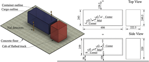
A 662-keV γ-radiation source was modeled as a 2.5-cm radius sphere (resembling a point source). In each simulation, the source was positioned either at the center of the cargo, in the corner of the cargo, or at the midpoint between the center and corner. These three positions are depicted in Fig. 1, and henceforth, are referred to as the center, corner, and mid positions, respectively. The energy 662 keV was used as it is the characteristic emission of ¹³⁷Cs, which has widespread use in medical and industrial applications.^[21] With greater than TBq activities of ¹³⁷Cs used within irradiator and inspection systems, there is potential for malicious actors to obtain ¹³⁷Cs in dangerous quantities. Demonstrating the MLEM PS method for 662-keV γ radiation serves as a proxy for detecting isotopes with emissions in a similar energy range. The characteristic γ energies of other isotopes commonly used in industrial radiography, such as ¹⁹²Ir, ⁶⁰Co, and ⁷⁵Se in TBq activities, range from 264.7 to 1332.5 keV, roughly the order of magnitude of 662-keV γ radiation from ¹³⁷Cs.^[22,23]

Assuming a container transit speed of 1.2 ms⁻¹, the simulations were repeated in 0.1 s time steps while the source was within 2.5 m of the RPM assembly center, resulting in 42 measurements per detector. The container transit speed used in this work, 1.2 ms⁻¹, was slower than the speed specified for testing spectroscopic RPMs in ANSI N42.38-2015 (Performance Criteria for Spectroscopy-Based Portal Monitors)^[24] of 2.2 ms⁻¹, but for a 20-ft container, the slower speed still results in the container being within the RPM for ~4.2 s, which is less than the ANSI N42.38-2015–specified 5-s occupancy time.

Depending on the cargo density, 10⁷ or 10⁸ particle histories were simulated in GEANT4 corresponding to 100- and 1000-MBq (1-GBq) sources. To test the performance at different source activities, the gross and 662-keV photopeak counts calculated from the simulations were rescaled linearly; the ¹³⁷Cs test activity recommended in ANSI N42.38-2015^[24] for an unshielded source is approximately 0.59 MBq, rising to 3.1 MBq for a shielded source. After rescaling the measurements to the desired activities (3 MBq or 10 MBq), background counts were added to each of the measurements by randomly sampling from Poisson distributions characterized by the background count rates given in Table I.

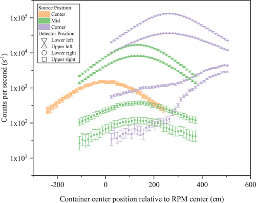
Figure 2 shows the simulated counts measured in the four panels of the PVT-based RPM as a function of container position, with the source in the center, mid, and corner positions and using 0.2 gcm${ }^{-3}$ cargo. The data for each source position were offset as measurements were only simulated when the source was within 2.5 m of the RPM center. Except when the source was in the corner position, the count distributions follow the expected pattern, which peaks when the source is in the center of the RPM. Order of magnitude differences in the counts were observed between the left- and right-side detectors when the source was in the mid and corner positions, which is due to the differences in the geometric efficiencies of the detectors and the amount of cargo between the source and each detector when the source was not in the center position. When the source was in the corner position, there was deviation from the expected shape of the count distribution for the right-side detectors. This results from there being significant shielding from the cargo until the back end of the container passes through the RPM, at which point the thickness of the cargo between the source and detector rapidly decreases. Particularly for the lower counts in Fig. 2, where there is more shielding material or a greater distance between the source and detector, some small-scale fluctuations are visible, arising from the stochastic nature of the Monte Carlo process in GEANT4.

Fig. 2. Simulated counts measured by four PVT scintillator detectors in an RPM as a shipping container passes through with a 10-MBq 662-keV source at the container center, mid, or corner position. Error bars are estimated from the square root of the number of counts, assuming Poisson counting statistics. The detector positions are defined similarly to Fig. 1, with two PVT detectors on either side of the container as opposed to four NaI detectors, and the source in the corner position is closest to the left-side detectors.

III.B. Detector Response Functions

To calculate the geometric ${ϵ}_G$ and intrinsic ${ϵ}_I$ efficiencies of the scintillator detectors, and the path lengths traversed by γ radiation through the container walls and cargo, an in-house Monte Carlo–based toolkit developed at the University of Bristol was used. The method involves defining the spatial region occupied by a cuboid scintillator, or the detector region, with intersecting planes. For any given source position, ${ϵ}_G$ of the detector is found by randomly sampling particle trajectories and determining the fraction that intersects the detector region using the Möller-Trumbore algorithm.^[25] By calculating the intersection points of each trajectory with the detector surfaces, the path length through the detector region is also derived. Combining the path lengths $l$ with the density $\rho$ of the scintillator material and its mass attenuation coefficient μ_g at 662 keV (see Table II), the attenuation factor, $\alpha =e^{-l{\mu }_g\rho }$, is calculated and averaged across all sampled particle trajectories to find $1-\bar{\alpha }$, which is ${ϵ}_I$ at 662 keV.^[4] The evaluation of ${ϵ}_I$ at 662 keV represents an approximation, as radiation may be scattered to lower energies in the cargo before being detected; the importance of this effect is expected to increase with the cargo density and is discussed in more detail in Secs. IV and V.

TABLE II Densities and Mass Attenuation Coefficients of Materials Used in This Work^[26]*

Material	Density (gcm^−3)	μg ($\times {10}^{-2}$) (cm^2g^−1)
Iron	7.874	7.346
NaI	3.667	7.395
PVT (C9H10)	1.032	8.356

*Mass attenuation coefficients are evaluated at 662 keV for each material.

The values of ${ϵ}_G$ and ${ϵ}_I$ for each detector are evaluated at a grid of regularly spaced points spanning 12 m along the direction of travel through the RPM. The shipping container is voxelized into 15 $\times$ 7 $\times$ 7 voxels, and at each time step, as the shipping container passes through the RPM, the voxel positions are recalculated and ${ϵ}_G$ and ${ϵ}_I$ are evaluated using linear interpolation on the aforementioned regular grid. The voxelization of the shipping container into 15 $\times$ 7 $\times$ 7 voxels was chosen to yield adequate resolution within the shipping container, with each 40.5 $\times$ 36.3 $\times$ 36.1 cm voxel representing ~0.2% of the container, without requiring prohibitive computation time. Investigations using finer or coarser voxelization are left for future work, before which optimization of the methods used to evaluate ${ϵ}_G$, ${ϵ}_I$, ${\bar{l}}^{cargo}$, and ${\bar{l}}^{wall}$ will be required to reduce computation time.

To determine the path lengths traversed by radiation emitted from each voxel through the container walls and cargo, the aforementioned method is edited. In this progression, the container and cargo are defined by intersecting planes and the particles are randomly sampled from the detector volume on a trajectory toward the voxel center. As before, path lengths through the container walls and cargo are determined using the calculated intersection points between the container and cargo planes and the particle trajectories. At each time step, weighted average path lengths through the container walls and cargo are calculated, with the weights determined by the inverse square law relationship between the voxel center and the particle start. With the path lengths appropriately considered, the full DRF for the j’th voxel at a particular time step is expressed as

(10) $\begin{array}{rl}& \mathrm{D}\mathrm{R}{\mathrm{F}}_j={ϵ}_j^G{ϵ}_j^{I}exp(-{\bar{l}}_j^{wall}{\rho }^{iron}{\mu }_g^{iron})\\ & exp(-{\bar{l}}_j^{cargo}{\rho }^{cargo}{\mu }_g^{cargo}),& (10)\end{array}$(10)

where ${\bar{l}}^{wall}$ is the average path length through the container walls, and ${\bar{l}}^{cargo}$ is the average path length through the cargo. The attenuating effect of air between the container and the detectors is not included in the DRF.

The use of ${\bar{l}}^{cargo}$ and ${\bar{l}}^{wall}$ is an approximation, and for some voxels, it is a poor one. For each voxel, the variation in path length through the cargo is assessed for the NaI-based RPM by considering the weighted mean and standard deviation of the path lengths. Typically, the standard deviation of the path lengths varies between 0% to 5% of the mean for the majority of voxels; however, for some voxels, the variance is greater than 50%, with the maximum observed standard deviation of 130% equivalent to 101 cm. Such variations in the path lengths highlight the drawback of using an average to describe them and will significantly hinder attempts to account for attenuation in the DRF, and as a result, will hinder the characterization of the source. The effect is expected to be even worse for the PVT-based RPM, where the larger detector cross sections result in higher variations in the path lengths. Compounding this effect is the use of the geometric mean of the attenuation factors $exp(-\overline{l_j}\rho {\mu }_g)$ rather than the arithmetic mean $\overline{exp(-l_j\rho {\mu }_g)}$, leading to an underestimation of the mean attenuation factor, which is equivalent to an overestimation of the amount of attenuation.

IV. RESULTS

Using the DRF, or $\mathbf{A}$, calculated as in Sec. III.B, and the simulated RPM measurements, or $\mathbf{y}$, described in Sec. III.A and shown in Fig. 2 for the PVT-based RPM, the iterative update equations [Eqs. (7)(7) ${\hat{\mathbf{x}}}^{k+1}=\frac{{\hat{\mathbf{x}}}^k}{{\mathbf{A}}^T\cdot \mathbf{1}}\otimes \left[{\mathbf{A}}^T\cdot \frac{\mathbf{y}}{\mathbf{A}\cdot {\stackrel{\mathbf{ˆ}}{\mathbf{x}}}^k+{\hat{b}}^k\mathbf{t}}\right]$(7) and (8)(8) ${\hat{b}}^{k+1}=\frac{{\hat{b}}^k}{{\mathbf{t}}^T\cdot \mathbf{1}}\left[{\mathbf{t}}^T\cdot \frac{\mathbf{y}}{\mathbf{A}\cdot {\stackrel{\mathbf{ˆ}}{\mathbf{x}}}^k+{\hat{b}}^k\mathbf{t}}\right],$(8) ] are used to find the optimum activity in a single voxel and the background count rate that explains the measurements $\mathbf{y}$. Following the approach in Ref. [10], the voxels are initialized with an activity calculated from the analytical solution to Eq. (4)(4) $\mathbf{Y}=\mathbf{A}\cdot \mathbf{x}+b\mathbf{t},$(4) without background: ${\mathbf{X}}_{initial}=\frac{{\mathbf{y}}^T\cdot \mathbf{1}}{{\mathbf{A}}^T\cdot \mathbf{1}}$. For all implementations of the MLEM PS algorithm, 30 iterations were performed; rather than set stopping criteria based on the change in $\mathrm{\ell }$ between iterations, a fixed number of iterations was chosen for consistency. The effects of overfitting, which are common in MLEM algorithms when the problem is underdetermined, are less prevalent in the MLEM PS method due to the constraint that the solution is in a single voxel.^[11]

IV.A. Characterizing the Source Without Cargo

First, the MLEM PS algorithm was applied to the source localization problem in the absence of cargo, i.e., ${\bar{l}}^{cargo}$ equal to zero in Eq. (10)(10) $\begin{array}{rl}& \mathrm{D}\mathrm{R}{\mathrm{F}}_j={ϵ}_j^G{ϵ}_j^{I}exp(-{\bar{l}}_j^{wall}{\rho }^{iron}{\mu }_g^{iron})\\ & exp(-{\bar{l}}_j^{cargo}{\rho }^{cargo}{\mu }_g^{cargo}),& (10)\end{array}$(10) . For the PVT-based RPM with the source in the corner position, the $\mathrm{\ell }$ values of the point-source solution that satisfy Eq. (6)(6) $\hat{\mathbf{x}},\hat{b}=\underset{\mathbf{x},b}{\mathrm{a}\mathrm{r}\mathrm{g}\mathrm{m}\mathrm{i}\mathrm{n}}\mathrm{\ell }(\mathbf{x},b|\mathbf{y}),$(6) in each voxel are illustrated in Fig. 3, with the lower $\mathrm{\ell }$ value voxels colored yellow. Note that the width axes in Figs. 3, 4, 8 and 9 are flipped. As expected, the best solutions are in the back right corner of the container, as shown in Fig. 3, and the point-source solutions are less likely in voxels farther away from this position. The smallest $\mathrm{\ell }$ solution was taken as the solution to the MLEM PS algorithm.

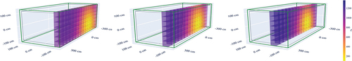
Fig. 3. Values of $\mathrm{\ell }$ (arbitrary units) calculated from the optimum point-source solution in each voxel when a 3-MBq source is in the corner position, there is no cargo (0.0 gcm⁻³), and measurements are with the PVT-based RPM. $\mathrm{\ell }$ is shown at three cross sections through the voxelized shipping container, and the smallest $\mathrm{\ell }$ values indicate the most likely source positions. The green box is the outline of the container.

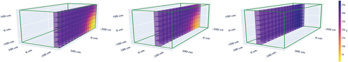
Fig. 4. Values of $\mathrm{\ell }$ (arbitrary units) calculated from the optimum point-source solution in each voxel when a 3-MBq source is in the center position, there is no cargo (0.0 gcm⁻³), and measurements are with the PVT-based RPM. $\mathrm{\ell }$ is shown at three cross sections through the voxelized shipping container, and the smallest $\mathrm{\ell }$ values indicate the most likely source positions. The green box is the outline of the container.

With the source in the corner (Fig. 3) and mid positions, the $\mathrm{\ell }$ values appear to vary smoothly, being smallest approximately around the true location of the source. Figure 4 shows that when the source is in the center position, the $\mathrm{\ell }$ values do not vary as smoothly, with the local minima in $\mathrm{\ell }$ observed at the center and sides of the container. The identification of any of these local minima as the point-source source solution could result in large localization errors. Such variations in $\mathrm{\ell }$ are attributed to the symmetry of the setup when the source is in the center and mean that degenerate solutions may exist.

Figure 5 shows the activity estimates, localization errors, and background count-rate estimates for the optimum point-source solution for each source position and detector type. Without cargo present, MLEM PS consistently localizes the source to within the dimensions of one voxel (40.5 $\times$ 36.3 $\times$ 36.1 cm) and estimates the activity to the correct order of magnitude. When the source is in the center position, MLEM PS localizes the source to the correct voxel for each data set, indicated by zero localization error.

Fig. 5. Algorithm (a) activity, (b) localization, and (c) background estimation performance for a 10-MBq 662-keV source at the center, mid, or corner of a 20-ft shipping container. Results are after 30 iterations, and the true background count rates are 100, 2000, and 5000 for the NaI photopeak (NaI PP), NaI gross (NaI), and PVT data, respectively, as indicated by the solid horizontal lines in (c). The true source activity, 10 MBq, is indicated by the solid line in (a), and the size of one voxel is 40.5 $\times$ 36.3 $\times$ 36.1 cm.

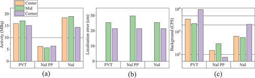
Figure 5a suggests that the use of gross-count and photopeak-count data sets results in an overestimation and underestimation of the source activities, respectively. Such an effect is explained by the nature of the DRF; the DRF describes the fraction of radiation emitted from the radioactive source that deposits energy in the detector without prior interactions in the cargo or container walls. The use of photopeak-count data is therefore expected to underestimate the activity, as they do not include events where radiation incident onto the detector deposits only a fraction of its energy. For the gross-count data, “buildup” radiation scattered into the detector from interactions in surrounding materials, such as the container walls, cargo, or air, means that the gross counts may result in overestimations of the activity. The effect of the gross-count data is expected to be worse when there is more cargo in the shipping container, as the fraction of scattered radiation incident on the detector is likely to be greater. Other reasons for the method to over- or underestimate the source activity include the method under- or overestimating the background count rate, under- or overestimating the amount of attenuation in the container walls [described by ${\bar{l}}^{wall}$ in Eq. (10)(10) $\begin{array}{rl}& \mathrm{D}\mathrm{R}{\mathrm{F}}_j={ϵ}_j^G{ϵ}_j^{I}exp(-{\bar{l}}_j^{wall}{\rho }^{iron}{\mu }_g^{iron})\\ & exp(-{\bar{l}}_j^{cargo}{\rho }^{cargo}{\mu }_g^{cargo}),& (10)\end{array}$(10) ], or not accounting for attenuation in air in the DRF.

IV.B. Characterizing the Source with Known Cargo

In this section, MLEM PS is used to find a point source concealed in a 0.2 gcm⁻³ and 0.6 gcm⁻³ iron cargo distributed homogeneously in the shipping container. The attenuating effect of the cargo is accounted for in the DRF, i.e., the ${\bar{l}}^{cargo}$ values calculated as described in Sec. III.B are used in the DRF, and the mass attenuation coefficient of the cargo is assumed known, 7.346 $\times$ 10⁻² cm²g⁻¹ for iron. As mentioned in Sec. IV.A, the presence of cargo increases the amount of (scattered) buildup radiation incident onto the detector, and therefore, the gross-count data are expected to result in an overestimation of the point-source activity.

Figures 6 and 7 illustrate the activity estimates, localization error, and background estimates for a concealed 10-MBq 662-keV source with the 0.2 gcm⁻³ and 0.6 gcm⁻³ iron cargo, respectively. At the lower cargo density (Fig. 6), the localization performance is consistently within 40.5 cm, the $x$-dimension of one voxel, and the activity estimates are in line with expectations described previously (over- and underestimated with gross-count and photopeak-count data, respectively). Moving to higher density cargo (Fig. 7), the NaI gross-count method fails to localize the source in the central position, which is attributed to the attenuation in cargo reducing the signal-to-noise ratio, such that the measured counts are diluted by the background as well as the nature of the solution when the source is in the center (as discussed in Sec. IV.A and shown in Fig. 4).

Fig. 6. Algorithm (a) activity, (b) localization, and (c) background estimation performance for a 10-MBq 662-keV source at the center, mid, or corner of a 20-ft shipping container containing a 0.2 gcm⁻³ iron cargo. Results are after 30 iterations, and the true background count rates are 100, 2000, and 5000 for the NaI photopeak (NaI PP), NaI gross (NaI), and PVT data, respectively, as indicated by the solid horizontal lines in (c). The true source activity, 10 MBq, is indicated by the solid lines in (a), and the size of one voxel is 40.5 $\times$ 36.3 $\times$ 36.1 cm.

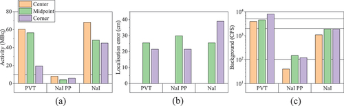
Fig. 7. Algorithm (a) activity, (b) localization, and (c) background estimation performance for a 10-MBq 662-keV source at the center, mid, or corner of a 20-ft shipping container containing a 0.6 gcm⁻³ iron cargo. Results are after 30 iterations, and the true background count rates are 100, 2000, and 5000 for the NaI photopeak (NaI PP), NaI gross (NaI), and PVT data, respectively, as indicated by the solid horizontal lines in (c). The true source activity, 10 MBq, is indicated by the solid lines in (a), and the size of one voxel is 40.5 $\times$ 36.3 $\times$ 36.1 cm.

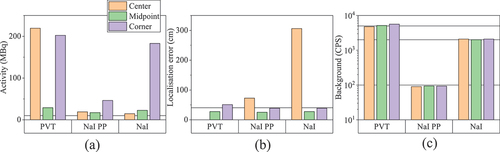
Figure 7 shows that the MLEM PS method grossly overestimates the activity when the source is at the center and corner positions for the PVT-based RPM and the corner position for the NaI-based RPM with gross counts. This is despite reasonable localization performance, and is not consistent with the activity estimation when the source is in the mid position for the gross-count data. Further work is required to investigate this difference. Overfitting is ruled out as a cause for this difference by implementing the algorithm for 2, 5, 10, 20, 30, and 40 iterations, which shows that the algorithm converges after roughly 5 to 10 iterations, but there is no significant change in activity in subsequent iterations while the localization error remains constant. For the case with the source in the center position, a step change in the activity and localization occurred between 20 to 30 iterations without significantly changing the likelihood, highlighting the presence of degenerate solutions when the source is in the center position and the PVT-based RPM is used.

As the cargo density increases, the estimates using the NaI photopeak data switch from underestimating the activity to overestimating the activity. Considering this, with the fact that the NaI photopeak data are expected to result in an underestimation of the activity, suggests that the method of accounting for attenuation in the cargo in the DRF is overestimating the amount of attenuation. Specifically, the value ${\bar{l}}_{cargo}$ is overestimating the characteristic distance traveled by radiation through the cargo. The effect is exacerbated at higher densities due to the exponential dependence of the DRF on the product of ${\bar{l}}_{cargo}$ and ${\rho }_{cargo}$.

For shielded sources, the ANSI N42.38-201 performance criteria for a spectroscopic RPM is 3 MBq for a ¹³⁷Cs source.^[23] Figures 8 and 9 show the $\mathrm{\ell }$ values for the NaI-based RPM gross-count and photopeak-count data, respectively, with the 3-MBq source in the mid position and the 0.2 gcm⁻³ cargo. With a 3-MBq source and a 0.6 gcm${ }^{-3}$ iron cargo, both the NaI- and PVT-based RPM data sets fail to localize the source in the center position. One factor affecting this is the aforementioned symmetric distribution of the source within the container and degenerate solutions when the source is in the center position. For the NaI RPM with photopeak-count data, the corner and mid position localization errors are within 40.5 cm, and the activities varied between 5.5 and 14.0 MBq, compared to 51.0 cm and 8.7 to 61.0 MBq for the PVT RPM.

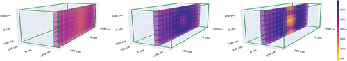
Fig. 8. Values of $\mathrm{\ell }$ (arbitrary units) calculated from the optimum point-source solution in each voxel when a 3-MBq source is in the mid position, there is a 0.2 gcm⁻³ iron cargo, and measurements are the gross counts with the NaI-based RPM. $\mathrm{\ell }$ is shown at three cross sections through the voxelized shipping container, and the smallest $\mathrm{\ell }$ values indicate the most likely source positions. The green and gray boxes are the outlines of the container and cargo, respectively.

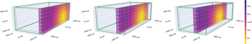
Fig. 9. Values of $\mathrm{\ell }$ (arbitrary units) calculated from the optimum point-source solution in each voxel when a 3-MBq source is in the mid position, there is a 0.2 gcm⁻³ iron cargo, and measurements are the photopeak counts with the NaI-based RPM. $\mathrm{\ell }$ is shown at three cross sections through the voxelized shipping container, and the smallest $\mathrm{\ell }$ values indicate the most likely source positions. The green and gray boxes are the outlines of the container and cargo, respectively.

IV.C. Characterizing the Source with Unknown Cargo

The previous section demonstrated how the source location, activity, and background count-rate estimation could be performed by incorporating the attenuating effect of the cargo into the DRF using Eq. (9)(9) $N_{ij}\sim \mathrm{P}\mathrm{o}\mathrm{i}\mathrm{s}\mathrm{s}\mathrm{o}\mathrm{n}(a_{ij}{e}^{-{\mu }_g\rho r_{ij}}{x}_j),$(9) . In practice, the attenuating effect of the cargo is characterized by μ_g and the density of the material in the cargo, both of which may be unknown. By assuming that the cargo is composed of a single material and homogeneously distributed at a constant, measurable density within the container, an attempt was made to quantify μ_g of the cargo by brute-force search. In the brute-force method, rather than substituting a single known value of μ_g into Eq. (9)(9) $N_{ij}\sim \mathrm{P}\mathrm{o}\mathrm{i}\mathrm{s}\mathrm{s}\mathrm{o}\mathrm{n}(a_{ij}{e}^{-{\mu }_g\rho r_{ij}}{x}_j),$(9) , a search over many possible μ_g values is performed, and the point-source solution and μ_g that yielded the solution with the lowest $\mathrm{\ell }$ value are taken to be the optimum solution. The background rate was assumed known, and simulated data from a 10-MBq 662-keV γ-radiation source was used.

Figure 10 shows the result of a brute-force search for the optimum point-source solution and μ_g using the PVT RPM with a 0.2 gcm⁻³ iron cargo; the search involved 50 potential μ_g values spaced between 0.04 and 0.155 cm²g⁻¹. The bottom row of graphs in Fig. 10 illustrates how the likelihood value for the optimum point-source solution varies as a function of μ_g, while the top two rows of graphs depict the localization error and activity of the optimum point-source solution. Step changes in the localization error indicate when the optimum point-source solution moves to a different voxel and corresponds to nonsmooth changes in the activity and likelihood.

Fig. 10. Brute-force implementation of MLEM PS with μ_g values in the range 0.008 to 0.031 cm⁻¹. The results are for a PVT RPM with a 10-MBq source concealed in a 0.2 gcm⁻³ iron cargo, with the source in the center (left column), mid (middle column), and corner (right column). The likelihood of the optimum solution, the activity, and the localization error are shown. The black dashed line represents μ_g at the optimum solution, and the red dashed line is the true μ_g.

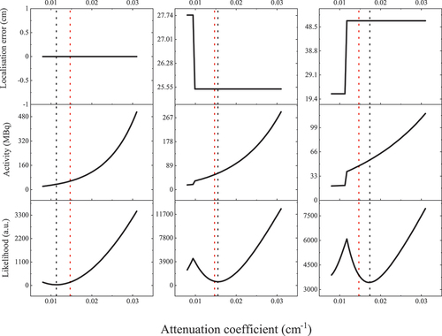
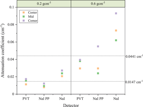
Figure 11 shows the optimum estimated attenuation factors in cm⁻¹ for each data set. The corresponding localization errors were less than 40.5 cm, except when the source was in the corner position with the PVT detector and when the source was in the center position with the 0.6 gcm⁻³ cargo for either NaI detector data set. The localization errors were all less than 73 cm, and when the localization error was less than 40.5 cm, the optimum activities varied from 5.8 to 125.0 MBq (55.0 to 366.0 MBq when $r_{err}$ was greater than 40.5 cm). Such results indicate reasonable localization performance and a similar spread of activities, as observed in Sec. IV.B. The ability of the method to estimate μ_g of the cargo is less promising. While μ_g values appeared to be clustered around the true value for the 0.2 gcm⁻³ cargo, this range of values, 0.040 to 0.136 cm²g⁻¹, covers a wide range of materials, including iron (0.074 cm²g⁻¹) and ethanol (0.087 cm²g⁻¹). For the 0.6 gcm⁻³ cargo, the spread of μ_g estimates were similar, ranging from 0.040 to 0.155 cm²g⁻¹.

Fig. 11. Optimum attenuation factors determined using MLEM PS and a brute-force search over possible attenuation factors for the gross-count PVT and NaI data sets and the NaI photopeak data set (NaI PP). The horizontal dashed lines represent the true attenuation factors in the 0.2 gcm⁻³ and 0.6 gcm⁻³ cargo in units of cm⁻¹.

V. DISCUSSION

In Secs. IV.A and IV.B, the MLEM PS method is used to characterize a 10-MBq 662-keV point source with homogeneous iron cargo at known densities of 0.0, 0.2, and 0.6 gcm⁻³. At the two lower densities, the method is capable of localizing the source to within the maximum dimension of one voxel, 40.5 cm, for every source position and achieves reasonable activity estimates. Factors, including a lower signal-to-noise ratio, the exponential dependence on the product of ${\bar{l}}_{cargo}$ and the density in the DRF, and buildup when using gross counts, contribute to the algorithm’s poorer performance with the 0.6 gcm⁻³ cargo. A loaded container density of 0.6 gcm⁻³ is around the upper mass limit for a loaded shipping container, with a small proportion of containers being this full.^[20] Adapting screening times to measure heavier containers for longer could provide a means of improving the signal-to-noise ratio in higher-density containers without introducing significant delays.

For the simulated data in this work, the MLEM PS method was capable of localizing a point source to within two voxels with data from the PVT- and NaI-based RPMs when μ_g of the cargo is unknown and the cargo density and distribution are known. However, the activity and μ_g estimates varied more significantly, with μ_g values covering a range of possible materials. This discrepancy between the true activity and μ_g values is due to a combination of factors. One factor is the use of photopeak-count and gross-count data, neither of which are fully compatible with the DRF but represent count rates that can be simply obtained from a measured spectrum. Future work could introduce a correction factor to the photopeak counts; division by the ratio of the photoelectric interaction cross section to the total interaction cross section of 662-keV γ’s in the detector may reduce the systematic underestimation of the activity using the photopeak-count data, although this ignores γ’s that deposit all their energy in the detector via multiple interactions.

The second factor is the calculation of the attenuation factors in the DRF; using a simple average to describe the path lengths through the cargo and walls fails to capture the true complexity of the scenario. As alluded to in Sec. IV.B, there is evidence that for the NaI detectors, the $exp(-{\bar{l}}^{cargo}{\rho }^{cargo}{\mu }_g^{cargo})$ term is being overestimated, which can be attributed to the poor characterization of ${\bar{l}}^{cargo}$. For the PVT detectors, the average value of the path length is expected to be a worse approximation since the larger panels subtend a greater solid angle of the emitted source distribution, making more paths between a voxel center and detector available. In medical applications and other related work where attenuation is modeled, this effect is significantly smaller as low-volume, point-like detectors (~1 cm³) are used, such that the path lengths through the attenuating material between each voxel and detector have a lower variance.^[12]

The use of collimation or a coded mask with the large area detectors used in conventional RPMs could provide part of the solution to this problem; however, intentionally shielding some of the large detector faces desirable for shipping container screening may decrease the overall detection efficiency of the RPM, which is the priority in shipping container screening. Since using the MLEM PS algorithm with known cargo yielded better results than with unknown cargo, it is worth considering what could be done to better characterize the cargo before the RPM screening process. Combining passive radiation measurements from NaI- and PVT-based RPMs with additional data streams is also necessary to account for the further degrees of freedom introduced by allowing cargo distribution and density to vary within the container.

Perhaps the most comprehensive method available for accounting for heterogeneous and composite cargo uses X-ray radiography to screen the cargo before passing through the RPM. Previous work has combined simple plastic scintillator–based RPM measurements of a shipping container carrying boxes of wood mulch and a 0.37-MBq ¹³³Ba source with a X-ray radiograph of the cargo to show that by accounting for the shielding with radiographic data, the localization error can be reduced from within 1 m to ~40 cm.^[17] Considering the results in Fig. 6, where the cargo composition was assumed known and homogeneous, the MLEM PS method achieved similar localization performance to the method in Ref. [17] with a radiograph for similar density cargo (0.2 gcm⁻³), though that work employed an order of magnitude lower activity source as well as a shorter transit time.

Instead of using X-ray radiography to estimate the material properties and density profile of containerized cargo, which requires investment in infrastructure, raises ethical issues, and can require greater than GBq sources of ⁶⁰Co or other isotopes, other potential information sources may be accessible. Most simply, the specified contents of the container could be used to estimate μ_g for the cargo, and combined with the cargo density calculated from the container mass, MLEM PS could be implemented to estimate the source parameters. Such a method would rely on accurate knowledge of the cargo contents, which may not be readily available, and assumes the trust and competence of the organization or individual consigning the cargo.

Alternatively, for nonhomogeneous cargo, information regarding the weight distribution of the cargo within the container may be attainable when the container is lifted from land to sea or visa versa. Incremental changes to the homogeneous cargo assumption could then be used to improve the model; for example, the center of mass (CoM) of the cargo could be calculated, and the cargo could be assumed to be uniformly distributed around the CoM in a regular shape.

Another constraining assumption in this work is that any concealed source could be approximated as a point source. In reality, concealed sources or NORM in a shipping container could be distributed through the container. In Ref. [11], the MLEM PS method was developed further to identify multiple point sources that might be present in the scene. In the case of large-volume radioactive sources, such as NORM shipments of cat litter or building materials/aggregates, the point-source method may fail to accurately describe the cargo. Here, the general MLEM method may be better suited to reconstructing these source distributions.

To continue the development of the MLEM image reconstruction approach to characterizing sources in shipping containers, further data are required. Future work should involve simulations of different source distributions to test the ability of MLEM PS and other variants of the MLEM algorithm to identify multiple point sources in a container and other nonpoint-like source distributions. Further reference cargo should also be defined and simulated to better represent the variety available in transiting shipping containers. A 2006 study of container imports through U.S. ports could form the basis for defining other common reference cargo.^[20] Finally, to test the reliability of the algorithm, the simulated data should be resampled and the algorithm repeatedly implemented to determine with what confidence the algorithm can repeatedly localize and predict the activity of concealed sources.

VI. CONCLUSIONS

A point-source variant of the MLEM algorithm, proposed in Ref. [11], was used to characterize point sources concealed within shipping containers using large-area, nondirectional PVT and NaI scintillator detectors found in existing shipping container screening infrastructure. Without cargo, the MLEM PS method was capable of localizing a 10-MBq 662-keV source to within 30.0 cm while estimating the activity and background count rate to the correct order of magnitude.

To include the effects of cargo attenuation in the DRF, the mean paths through the cargo were calculated for each voxel within the shipping container at 0.1-s intervals as the container passed through the RPM. Assuming the cargo composition is known and distributed homogeneously throughout the container, the MLEM PS method was capable of localizing a 3-MBq 662-keV source with both the PVT- and NaI-based scintillators, except when the source was at the container center and the cargo density was 0.6 gcm⁻³, close to the cargo mass limit for a shipping container.

Where MLEM PS failed to localize the source was partly attributed to the added background counts being of the same order of magnitude to the measurements. Since conservative estimates of the background were used, in practice the method may be capable of localizing the source at all simulated positions and densities.

When the material composition of the cargo is not known, but the background is fixed, the MLEM PS method was generally still capable of localizing a 10-MBq 662-keV source to within 73.0 cm and estimating the activity to within one order of magnitude with both the NaI photopeak-count and PVT gross-count data. Estimates of μ_g characterizing the cargo material were less accurate, and using the methodology in this work, could not be used to differentiate between common cargo. It may be possible to improve the estimates of μ_g by calculating better estimates of the uncollided 662-keV flux incident onto the detector; however, this would only be feasible with photopeak data since the buildup in the gross-count data cannot be fully accounted for without a full description of the cargo. Accounting for attenuation in air may also lead to more accurate results, although this would require the calculation of the mean path lengths through air, and as has been discussed throughout this work, the use of a mean path length to characterize the attenuation is perhaps the largest limiting factor in accurately determining μ_g.

This work demonstrates how the MLEM PS method could be implemented on existing shipping container screening infrastructure at seaports to provide information regarding the location of a concealed point source within a container. If prior knowledge of the container contents and density was obtained, the method might also allow for the activity of the source to be estimated. Such capability results in a significantly reduced search area in secondary screening procedures of shipping containers at seaports using existing infrastructure, which is predominantly PVT-based RPMs. Additional work is required to test the algorithm with multiple and nonpoint-like sources and to explore how the DRF can be edited to account for different, common reference cargo.

Acknowledgments

Additional acknowledgement is given to the Royal Academy of Engineering, Dr. Sam White, and the University of Bristol’s Jean Golding Institute for their assistance in and funding for this work.

Disclosure Statement

No potential conflict of interest was reported by the author(s).

Additional information

Funding

Financial support for Euan Connolloy’s PhD project is provided by the Atomic Weapons Established (AWE) and STFC-AWE funded Nuclear Security Network under project reference ST/S005684/1. Dean Connor acknowledges funding from the National Nuclear Laboratory Core Science Decontamination Science Theme and U.K. Research and Innovation through the National Center for Nuclear Robotics (EP/R02572X/1).

References

- B. D. GEELHOOD et al., “Overview of Portal Monitoring at Border Crossings,” 2003 IEEE Nuclear Science Sym. Conference Record (IEEE Cat. No.03CH37515), 1, 513, Institute of Electrical and Electronics Engineers (2008); https://doi.org/10.1109/nssmic.2003.1352095.
- E. L. CONNOLLY and P. G. MARTIN, “Current and Prospective Radiation Detection Systems, Screening Infrastructure and Interpretive Algorithms for the Non-intrusive Screening of Shipping Container Cargo: A Review,” J. Nucl. Eng., 2, 3, 246 (2021); https://doi.org/10.3390/jne2030023.
- R. T. KLANN, J. SHERGUR, and G. MATTESICH, “Current State of Commercial Radiation Detection Equipment for Homeland Security Applications,” Nucl. Technol., 168, 1, 79 (2009); https://doi.org/10.13182/nt09-a9104.
- R. HEVENER, M. S. YIM, and K. BAIRD, “Investigation of Energy Windowing Algorithms for Effective Cargo Screening with Radiation Portal Monitors,” Radiat. Meas., 58, 113 (2013); https://doi.org/10.1016/j.radmeas.2013.08.004.
- G. R. GILMORE, Practical Gamma-Ray Spectrometry, Vol. 52, John Wiley & Sons, Ltd. (2008); https://doi.org/10.1016/s0584-8539(96)90113-0.
- B. D. MILBRATH et al., “Radiation Detector Materials: An Overview,” J. Mater. Res., 23, 10, 2561 (2008); https://doi.org/10.1557/jmr.2008.0319.
- D. C. STROMSWOLD et al., “Field Tests of a NaI(Tl)-Based Vehicle Portal Monitor at Border Crossings,” IEEE Symposium Conference Record Nuclear Science 2004, 1, 196, Institute of Electrical and Electronics Engineers (2005); https://doi.org/10.1109/nssmic.2004.1462180.
- R. T. KOUZES et al., “Spectroscopic and Non-spectroscopic Radiation Portal Applications to Border Security,” IEEE Nuclear Science Symposium Conference Record, 1, 321, Institute of Electrical and Electronics Engineers (2005); https://doi.org/10.1109/NSSMIC.2005.1596262.
- U. SHIRWADKAR et al., “Low-Cost, Multi-Mode Detector Solutions,” Nucl. Instrum. Methods Phys. Res., Sect. A, 954, 161289 (2020); https://doi.org/10.1016/j.nima.2018.09.124.
- N. DINAR et al., “Pulse Shape Discrimination of CLYC Scintillator Coupled with a Large SiPM Array,” Nucl. Instrum. Methods Phys. Res., Sect. A, 935, 35, 35 (2019); https://doi.org/10.1016/J.NIMA.2019.04.099.
- D. HELLFELD et al., “Gamma-Ray Point-Source Localization and Sparse Image Reconstruction Using Poisson Likelihood,” IEEE Trans. Nucl. Sci., 66, 9, 2088 (2019); https://doi.org/10.1109/TNS.2019.2930294.
- M. S. BANDSTRA et al., “Improved Gamma-Ray Point Source Quantification in Three Dimensions by Modeling Attenuation in the Scene,” IEEE Trans. Nucl. Sci., 68, 11, 2637 (2021); https://doi.org/10.1109/TNS.2021.3113588.
- J. FESSLER, “Space-Alternating Generalized EM Algorithms for Penalized Maximum-Likelihood Image Reconstruction,” p. 1, University of Michigan Ann Arbor (1994); http://www.eecs.umich.edu/techreports/systems/cspl/cspl-286.pdf.
- A. KROL et al., “An EM Algorithm for Estimating SPECT Emission and Transmission Parameters from Emission Data Only,” IEEE Trans. Med. Imaging, 20, 3, 218 (2001); https://doi.org/10.1109/42.918472.
- S. AGOSTINELLI et al., “Geant4—A Simulation Toolkit,” Nucl. Instrum. Methods Phys. Res., Sect. A, 506, 3, 250 (2003); https://doi.org/10.1016/S0168-9002(03)01368-8.
- K. D. JARMAN et al., “Bayesian Radiation Source Localization,” Nucl. Technol., 175, 1, 326 (2011); https://doi.org/10.13182/NT10-72.
- E. A. MILLER et al., “Combining Radiography and Passive Measurements for Radiological Threat Localization in Cargo,” IEEE Trans. Nucl. Sci., 62, 5, 2234 (2015); https://doi.org/10.1109/TNS.2015.2474146.
- P. H. HENDRIKS, J. LIMBURG, and R. J. de MEIJER, “Full-Spectrum Analysis of Natural γ-Ray Spectra,” J. Environ. Radioact., 53, 3, 365 (2001); https://doi.org/10.1016/S0265-931X(00)00142-9.
- “Series 1 Freight Containers—Classification, Dimensions and Ratings,” ISO 668, International Organization for Standardization (2020); https://www.iso.org/standard/76912.html.
- M. DESCALLE, D. MANATT, and D. SLAUGHTER, “Analysis of Manifests for Containerized Commodities Imported through US Ports,” 2006 IEEE Nuclear Science Symposium Conference Record, 1, 275 (2006); https://doi.org/10.1109/NSSMIC.2006.356155.
- “Categorization of Radioactive Sources,” IAEA Safety Standards Series, No. RS-G-1, p. 70, International Atomic Energy Agency (July 2005); https://www.iaea.org/publications/6808/categorization-of-radioactive-sources.
- “SENTINEL 880 Series Gamma-Ray Source Projectors,” QSA Global, Inc; https://www.qsa-global.com/880-series-gamma-ray-source-projectors ( accessed Dec. 20, 2022).
- “Live Chart of Nuclides,” Nuclear Data Section, International Atomic Energy Agency; https://www-nds.iaea.org/relnsd/vcharthtml/VChartHTML.html ( accessed Dec. 20, 2022).
- “American National Standard for Performance Criteria for Spectroscopy-Based Portal Monitors Used in Homeland Security,” ANSI N42.38-2015 (Rev. of ANSI N42.38-2006), pp. 1–59, (Jan. 29, 2016); https://doi.org/10.1109/IEEESTD.2016.7394937.
- T. MÖLLER and B. TRUMBORE, “Fast, Minimum Storage Ray-Triangle Intersection,” J. Graphics Tools, 2, 1, 21 (1997); https://doi.org/10.1080/10867651.1997.10487468.
- K. O. M. J. BERGER et al., “XCOM: Photon Cross Sections Database,” National Institute of Standards and Technology; https://www.physics.nist.gov/PhysRefData/Xcom/html/xcom1-t.html ( accessed Oct. 22, 2022).