Examination of Deep Learning Algorithm for Nuclear Proliferation Risk Modeling

Abstract

Previous studies have explored the determinants of the nuclear proliferation levels (Explore, Pursue, and Acquire). However, these studies have weaknesses, including endogeneity and multicollinearity among the independent variables. This resulted in tentative predictions of a country’s nuclear program capabilities. The objective of this study is to develop a tool to predict future nuclear proliferation in a country, and thus facilitate its prevention. Specifically, we examine how applying deep learning algorithms can enhance nuclear proliferation risk prediction. We collected important determinants from the literature that were found to be significant in explaining nuclear proliferation. These determinants include economics, domestic and international security and threats, nuclear fuel cycle capacity, and tacit knowledge development in a country. We used multilayer perceptrons in the classification model. The results suggest that detecting a country’s proliferation behavior using deep learning algorithms may be less tentative and more viable than other existing methods. This study provides a policy tool to identify a country’s nuclear proliferation risk pattern. This information is important for developing efforts/strategies to hamper a potential proliferating country’s attempt toward developing a nuclear weapons program.

Keywords:

• Nuclear proliferation
• predictive modeling
• multilayer perceptrons

I. INTRODUCTION

Why have countries explored, pursued, or acquired a nuclear weapons program? Nuclear weapon proliferation has been a major concern of the international community since the dawn of the nuclear age. In particular, with the growth in global electricity demand and the concern over climate change, interest in nuclear power is on the rise around the world. As nuclear technology has become commonplace,^[1] the potential for nuclear technologies to be used for both civil and military purposes could lead to possible nuclear proliferation attempts by countries in the future. As a result, the prediction, and by extension, the prevention of nuclear proliferation is a necessity in the continued growth of nuclear energy, and more generally, technology.

Many scholars have studied the causes and consequences of nuclear proliferation to prevent the risk of proliferation in the future. A number of studies have identified the factors that are significant in determining both attempts, and eventual successes, in nuclear proliferation.^[2–10] The determinants can be broadly divided into four categories: technological capability, external environments, domestic environments, and the nuclear nonproliferation norm. The logic of technological determinants is that a country’s ability to acquire nuclear weapons, and the duration of those efforts, requires (1) a certain level of economic output to afford nuclear weapons, (2) a certain level of scientific development and research capabilities to know how to develop, build, and deploy nuclear weapons, and (3) an industrial base with certain capabilities, notably the nuclear fuel cycle, to be able to produce the materials necessary for nuclear weapons.^{[4–8,11,12]}

Technical capacity, both in terms of knowledge and in terms of elements of the nuclear fuel cycle, may be aided by receiving nuclear assistance from other countries.^[6,7] But purposeful, formal nuclear cooperation is not the only way to acquire the know-how for nuclear programs: the indigenization of nuclear weapons technology through tacit knowledge development and transfer may affect the duration and success of nuclear proliferation programs.^[13–16] Hastings et al.^[13] examined the difference in nuclear-related research networks between Iran and Pakistan. They posit that nuclear research collaboration networks play a significant role in explaining the ability of a country to acquire and integrate the tacit knowledge necessary for nuclear proliferation. Through a social network analysis comparison between Iran and Pakistan, they found that the existence of dense and interconnected research clusters among individual researchers increases the success of the nuclear program in a country.^[13] Following this research, Baxter^[17] tested the influence of epistemic networks related to nuclear fuel cycle research on proliferation outcomes by using large-N regression analyses. He suggests that diameter, density, clustering coefficient, and diffusion variables gained from the social network analysis of nuclear fuel cycle research networks in a country are significant factors for explaining nuclear proliferation risk.

By contrast, the external and domestic environments of a country are determinants of a nation’s motivation rather than its capacity to build nuclear weapons; although, clearly, sufficient motivation is likely to influence a country’s push to develop nuclear capacity.^[4] In the external environment, proliferation risk depends on a country’s military partners and the nature of those partnerships, such as whether the country benefits from a nuclear umbrella and from military alliances. Without strong military alliances with nuclear-armed states, a country may be more likely to pursue nuclear weapons.^[5] Regarding domestic environments, a country’s political environment (although whether democracy or autocracy leads to nuclear proliferation is still controversial), popular support for nuclear weapons, state bureaucracy, liberal economic policies, the number of veto players in political decision making, and the leaders’ will to maintain power all can influence motivation to develop nuclear weapons.^[4,5]

Meanwhile, nonproliferation norms are able to prevent the pursuit of nuclear weapons, even if a country is an environment that would otherwise favor developing such nuclear weapons. The development of, and membership in, various nonproliferation treaties, from the Nuclear Nonproliferation Treaty (NPT) to the Additional Protocol, have been found to be significant in reducing nuclear proliferation risks.^[11]

However, accurately identifying determinants of nuclear proliferation can be hampered by model selection. Econometrics is a statistical tool based on the estimation and inference of causal effects. To investigate causality using econometrics, different models should be run to find the best fit model to explain the hypothesis authors have suggested. Each function of general regression or principled models (such as Weibull and Cox) is expected to be consistent with a given data set, thereby drawing a suitable coefficient to interpret causal effects.

Previous studies have examined the determinants of nuclear proliferation by using different statistical models (i.e., multinomial logistic regression, probit regression, Cox/Weibull Survival, and hazard models) and different sets of determinants (see Table I). Each paper identified different factors that result in increasing nuclear proliferation. However, there are issues of multicollinearity and endogeneity among independent variables that are likely to be significant when it comes to explaining nuclear proliferation. For instance, the security threat environment is likely to be correlated with the provision (and acceptance) of sensitive nuclear assistance, and a country’s economic capability is likely to be correlated with the presence of at least some parts of the nuclear fuel cycle.

TABLE I Comparison of the Models Included in the Literature on Proliferation Determinants

	Variables
Authors	Domestic Environment	External Environment	Nonproliferation Norms	Technological Capacity
				Economic/Technical Capability	Nuclear Assistance	Nuclear Fuel Cycle	Tacit Knowledge
Singh and Way^[Citation4]	X	X		X
Jo and Gartzke^[Citation5]	X	X	X	X
Fuhrmann^[Citation6]	X	X	X	X	X
Kroenig^[Citation7]	X	X	X	X	X
Li et al.^[Citation8]	X	X	X	X		X
Brown and Kaplow^[Citation9]	X	X	X	X	X
Bell^[Citation10]	X	X	X	X	X
Baxter^[Citation17]	X	X		X			X

Most of the existing literature using large-N analysis focuses on which determinants of proliferation best explain the cause and consequences of proliferation; the literature is not intended to enhance prediction modeling or to develop prediction methods. In that sense, Bell^[10] points out that most variables that the literature considers as significant factors fail to offer strong explanations for existing patterns of proliferation and do not provide much predictive capacity on proliferation levels. In one exception, which may show the way forward, Kaplow and Gartzke^[18] examined the predictive power of nuclear proliferation models by using a statistical learning method that finds that having a nuclear-armed rival is the strongest predictor of a state moving from nuclear latency to nuclear weapons status.

In this paper, we take a step toward overcoming some of the difficulties encountered in predicting and explaining proliferation levels in previous literature by using a deep learning algorithms framework to enhance predictive capability. Specifically, we use the Multilayer Perceptron (MLP) algorithm on a deep learning approach to classifying proliferation levels. Building on previous literature, we incorporate into our models most of the variables that have been identified as significant factors in proliferation and use them to overhaul predictive capacity. We find that machine learning, specifically a method using deep learning algorithms, has superior predictive capacity compared to standard econometrics-based models of proliferation.

The remainder of this study is organized as follows. In Sec. II, we describe our data and detail the operation of deep learning methods, and in Sec. III, we present our main results, which indicate the improved predictive capacity of our model. In Sec. IV, we discuss and cross validate the results, and apply our method to two important cases of proliferation: North Korea and Iran. Finally, in Sec. V, we conclude with a summary of the contributions of our research.

II. DEEP LEARNING METHODS

II.A. Data Set: Label and Features

A historical timeline of the worldwide spread of nuclear weapon programs was initially defined by Singh and Way.^[4] They designated each country’s nuclear weapons program in three levels: Explore, Pursue, and Acquire. More recently, Bleek^[19] updated the timeline of a country’s nuclear program based on new sources and evidence. According to Bleek’s data set,^[19] 31 countries have at least explored nuclear weapons programs. Among these countries, 17 countries have pursued development and 10 countries have acquired nuclear weapons (see Table II).

TABLE II Timeline of Nuclear Proliferation of a Country Coded by Bleek^[19]

Country	Explore	Pursue	Acquire
United States	1939–	1942–	1945–
Russia	1942–	1943–	1949–
United Kingdom	1940–	1941–	1952–
France	1945–	1954–	1960–
China	1952–	1955–	1964–
Israel	1949–	1955–	1967–
South Africa	1969–1991	1974–1991	1979–1991
Pakistan	1972–	1972–	1987–
India	1948–	1964–1966, 1972–1975, 1980–	1987–
Korea, North	1962–	1980–	2006–
Yugoslavia	1949–1962, 1974–1987	1953–1962, 1982–1987
South Korea	1969–1981	1970–1981
Libya	1970–2003	1970–2003
Brazil	1966–1990	1975–1990
Iraq	1975–1991	1975–1990
Iran	1974–1979, 1984–	1989–
Syria	2000–	2002–2007
Germany	1939–1945
Japan	1941–1945, 1967–1972
Switzerland	1945–1969
Sweden	1945–1970
Norway	1947–1962
Egypt	1955–1980
Italy	1955–1958
Australia	1956–1973
Germany, West	1957–1958
Indonesia	1964–1967
Taiwan	1967–1976, 1987–1988
Romania	1978–1989
Argentina	1978–1990
Algeria	1983–1991

Our data set is structured as a pooled time series, with the country-year as each observation. The labeling of each data point was implemented by using Bleek’s^[19] proliferation timelines from 1945 to 2000. That is, each observation label in our data set represents the nuclear proliferation level of each country in a given year. Therefore, the label of each observation to be used in our deep learning algorithm was dealt with as a multiclass, coded as No Interest, Explore, Pursue, and Acquire. The description of this labeling is shown in Table III.

TABLE III Description of the Label in the Time Series Data Set

Multiclass Label	Class Code	Description
No Interest	0	States without any interest in developing a nuclear weapons programs in a given year
Explore	1	Leaders of the state are opening the door to a potential nuclear weapons program in a given year
Pursue	2	Active programs are ongoing, authorized by leaders with the aim of acquiring nuclear weapons or the capacity to construct them on short notice in a given year.
Acquire	3	States obtaining at least rudimentary deliverable nuclear explosive devices in a given year

From Sagan,^[3] Singh and Way,^[4] to Baxter,^[17] many scholars have identified different sets of features that could affect the proliferation decision and duration of a country. Not only technological (including industrial and economic variables), external (international security), and internal (domestic politics) determinants, but also other factors, such as nuclear fuel cycle capability, research networks, and proliferation norms, have been highlighted in previous literature.

In light of the literature review discussed in Sec. I, we incorporated all the features that were used in previous nuclear proliferation literature. A total of 41 features were chosen under the new set of determinants and used as the input for the deep learning algorithm. They are summarized in Table IV.

TABLE IV Model Features

Variable	Description	Source	Range
Economic/Technical Capability Category
Gross domestic product per capita	Purchasing power parity gross domestic product per capita	Ref. [4]	Numeric
Gross domestic product	Gross domestic product	Ref. [8]	Numeric
Industrial capacity	Binary indicator including the threshold value of domestic steel production, electricity generation capacity, and energy consumption of a country	Ref. [4]	0/1
Composite index of capabilities	The composite index of capabilities is a measure of a state’s power, including population, iron and steel production, energy consumption, military expenditure, and military personnel.	Ref. [20]	0 to 1
Nuclear Fuel Cycle Capability Category
Uranium ore production	Uranium ore processing capability (tonnes of uranium per year)	Ref. [8]	Normalized from 0 to 1 (All values are divided by the maximum value of each variable.)
Uranium conversion capability	Uranium conversion capability (tonnes of heavy metal per year)	Ref. [8]
Uranium enrichment capability	Uranium enrichment capability (tonnes of separative work unit per year)	Ref. [8]
Uranium oxide fuel fabrication capability	Uranium oxide fuel fabrication capability (tonnes heavy metal per year)	Ref. [8]
Mixed-oxide fuel fabrication capability	Mixed-oxide fuel fabrication capability (tonnes heavy metal per year)	Ref. [8]
Wet spent fuel storage facility	Away-from-reactor wet spent fuel storage (tonne heavy metal)	Ref. [8]
Dry spent fuel storage facility	Away-from-reactor dry spent fuel storage (tonnes of heavy metal)	Ref. [8]
Spent fuel reprocessing capability	Spent fuel reprocessing capability (tonnes of heavy metal per year)	Ref. [8]
Zirconium alloy processing capability	Zirconium alloy processing capability (tonnes per year)	Ref. [8]
Zircaloy tube fabrication capability	Zircaloy tubing fabrication capability (tonnes per year)	Ref. [8]
Heavy water production capability	Heavy water production capability (tonnes per year)	Ref. [8]
Power reactor capacity	Electricity generation from commercial nuclear reactors [MW(electric)]	Ref. [8]
Number of all reactors	Number of all kinds of reactors	Ref. [8]
Number of fast reactors	Number of fast research reactors	Ref. [8]
Number of heavy water research reactors	Number of heavy water research reactors	Ref. [8]
Number of graphite research reactors	Number of graphite research reactors	Ref. [8]
Number of light water research reactors	Number of light water research reactors	Ref. [8]
Number of other types of research reactors	Number of other types of research reactors	Ref. [8]
Latency level	Variable indicating whether a state had an enrichment or reprocessing plant in operation: 2 if a state had pilot-scale plants of enrichment/reprocessing plants (including weapon possession), 1 if a state had at least laboratory-scale plants of enrichment/reprocessing plants, and 0 if state did not have any of them.	Ref. [21]	0/1/2
Nuclear Assistance Category
Sensitive nuclear assistance	Binary variable whether the state had an experience in receiving sensitive nuclear technologies (i.e., plutonium reprocessing, uranium enrichment) up to that year	Ref. [22]	0/1
Civilian nuclear assistance	Binary variable whether the state had an experience in receiving civilian nuclear assistance up to that year	Ref. [12]	0/1
Cumulative total number of civilian nuclear assistance	Cumulative number of the civilian nuclear assistance that the state had received or transferred up to that year	Ref. [12]	Numeric
Security/Threat Environment Category
Disputes	5-year moving average of the number of militarized interstates per year in which a state is involved	Ref. [4]	Numeric
Rivalry	Binary indicator whether a state was involved in one or more enduring rivalries in a given year	Ref. [4]	0/1
Allies	Binary indicator whether a state has a security guarantee in the form of a defense pact from a nuclear-armed power states (United States, Soviet Union/Russia, China, France, United Kingdom)	Ref. [4]	0/1
Centdems	The percentage of states each year that receive a score of 7 or higher on the Polity IV measure	Ref. [4]	Numeric
Domestic Environment Category
Polity	Polity IV score ranging from −10 to 10 indicating the level of autocracy (−10) to democracy (10)	Ref. [4]	−10 to 10
Openness	Exports plus imports as a share of gross domestic product	Ref. [4]	Numeric
Liberalization	5-year change in Openness variable	Ref. [4]	Numeric
Nonproliferation Norms Category
IAEA membership	Binary indicator whether a state was a member of IAEA at that year	Ref. [23]	0/1
NPT membership	Binary indicator whether a state was a member of the NPT	Ref. [5]	0/1
Safeguard	Binary indicator whether a state ratified the traditional IAEA safeguards (i.e., comprehensive safeguards agreements)	Ref. [8]	0/1
Additional protocol	Binary indicator whether a state has ratified additional protocol	Ref. [24]	0/1
Tacit Knowledge Environment Category
Network size	Diameter reachable (the distance between the nodes farthest from each reachable node) of a social network related to nuclear fuel cycle research	Ref. [17]	Numeric
Network density	Ratio of the number of links versus maximum possible links for a nuclear fuel cycle research network	Ref. [17]	0 to 1
Network clustering	Clustering coefficient measured by social network related to a nuclear fuel cycle research	Ref. [17]	0 to 1
Network diffusion	Ratio of the distance between entities in a network related to nuclear fuel cycle research	Ref. [17]	0 to 1

II.B. Deep Learning Algorithms: MLP

To improve upon preexisting models of nuclear proliferation, we introduced deep learning algorithms for the prediction capability of nuclear proliferation levels. Deep learning is a subfield of machine learning. In existing machine learning approaches, an expert must analyze and decide which feature to extract from among the various features of the data to be used. In deep learning, however, the machine learns by automatically extracting features from the data it wants to learn.^[25]

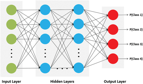
Deep learning algorithms are artificial neural networks that consist of interconnected neurons that are organized in layers. We specifically use MLP, one of the neural network architectures. The MLP model is a class of feedforward artificial neural networks with no recurrent connections. The MLP model consists of the input layer, hidden layers, and output layers. As shown in Fig. 1, MLP demonstrates a multilayer, fully connected neural network. Each neuron unit in a layer is connected to all neuron units of the previous and following layers, and each connection between the neurons has its weight. Therefore, the output of neurons in each layer is

(1) $\mathrm{y}=\mathrm{f}(\sum _i{x}_i{w}_i+b),$(1)

Fig. 1. MLP used in this study.

where $x_i$ is the input data or the outputs of other neurons, $w_i$ is the strength of the input neuron $\mathrm{i}$, and b is the bias value. In this study, we used a total of six layers, which included one input layer, four hidden layers, and one output layer.

Since the hidden layers exist between the input and output layers in the MLP model, it is important to define the weight of the nodes in the artificial neural network. Deep learning uses back-propagation, which is the process of updating the weights of nodes in each layer in a direction such that the model can make better predictions (direction to reduce loss values by calculating the distance between the prediction and the correct answer).^[26]

II.C. Activation Function and Batch Normalization

As shown in Eq. (1(1) $\mathrm{y}=\mathrm{f}(\sum _i{x}_i{w}_i+b),$(1) ), each neuron in a layer has its own activation function $f$ for determining its output value. If the activation function is not included in the model, the neural network will be stacked up by the combination of linear functions, which becomes just a linear function. In other words, the network will be the same as a linear regression model, which cannot classify linearly inseparable classes. Therefore, to catch nonlinear patterns in our nuclear proliferation data set, we used nonlinear activation functions for the output values of the neurons in each layer. There are various types of nonlinear activation functions, such as sigmoid, hyperbolic tangent, and rectified linear unit (ReLU). Since the range of the sigmoid and hyperbolic tangent is (0,1) and (−1,1), respectively, the vanishing gradient problem is encountered when we use one of them. In the process of back-propagation, the process of multiplying the differential value of the activation function is performed. In the case of the sigmoid or hyperbolic tangent functions, there is a large disadvantage in that the differential value is highly likely to be lost during gradient back-propagation.^[26] If the weights are not updated properly through the learning process, the optimal classification model cannot be found. Therefore, to solve the vanishing gradient problem in a neural network, we used ReLU [range is (0, ∞)] for the activation function in each layer in this study.

We also used batch normalization in our model to reduce the vanishing gradient and internal covariate shift problems.^[27] Batch normalization refers to the operation of normalizing the output value of the activation function of the layer in the MLP model. Through this process, deep learning could accelerate the learning speed. It could also prevent overfitting problems.

II.D. Softmax Function and Cross-Entropy Loss

Since there are four classes of outcomes in this analysis (No Interest, Explore, Pursue, and Acquire), we used a Softmax function for the final output layer in the MLP. The Softmax function is a generalized function for multiclass classification. It transforms the output layer values into the probability of each class by using

(2) $p_k=\frac{\mathrm{e}\mathrm{x}\mathrm{p}\left(y_k\right)}{{\sum }_{i=1}^n\mathrm{e}\mathrm{x}\mathrm{p}\left(y_i\right)},$(2)

where n is the number of classes (in this study, the number of classes is four), and $y_k$ represents the real value of the output layer. This function makes the sum of all the transformed outputs add up to 1.

In addition, we used a cross-entropy loss function to calculate the loss score in this study. The loss function in deep learning measures how the predicted results from the model deviate from the actual value. Specifically, for classification models, the cross-entropy loss function compares the difference between estimated class probabilities and actual class distribution. In one hot-encoded vector (actual class distribution), the real class label would have a probability of 1 and all others would have a probability of 0. The equation of the cross-entropy function is

(3) $\mathrm{C}\mathrm{r}\mathrm{o}\mathrm{s}\mathrm{s}-\mathrm{e}\mathrm{n}\mathrm{t}\mathrm{r}\mathrm{o}\mathrm{p}\mathrm{y}\mathrm{L}\mathrm{o}\mathrm{s}\mathrm{s}=-\sum _k{t}_{k}log{p}_k,$(3)

where $p_k$ is the probability output value of a model in class $k$, and $t_k$ is the corresponding target value of the one hot-encoded vector in class $k$.

II.E. Optimization

Optimization is a series of processes to find the minimum value of the loss function, thereby maximizing the accuracy of the output. Training a model in deep learning is actually the same as performing an optimization task to set the weight of each neuron in the network. Optimization proceeds while updating the weights during the back-propagation process. In our study, the process of the MLP model is ultimately to minimize the cross-entropy loss value by using an appropriate optimizer.

Gradient descent is the basic optimization method in deep learning algorithms. The method is based on descending a slope in the loss function graph to find the point with the minimum loss value.^[26] Due to the slow training speed of the gradient descent method in a big data set, various alternative types of optimizers have also emerged. In this study, we used the Adaptive Moment Estimation (ADAM) optimizer, which is fast and better with sparse gradients compared to the stochastic gradient descent optimizer.^[26]

II.F. Data Arrangement: Case, Batch, and Epoch

We used time series data of all countries from World War II to the year 2000 that could be aggregated to examine the classification model. Moreover, we dropped all observations from the data once a state acquired nuclear weapons (United States in 1945, Russia in 1949, United Kingdom in 1952, France in 1960, China in 1964, Israel in 1967, South Africa in 1979-91, Pakistan in 1987, and India in 1987).^a However, in the case of South Africa, which is the only country that ended a successful nuclear program, it reentered the data set after its program ended in 1992. In our data set, 4587 data points (a total of 119 countries) were used.

We divided the data set into training, validation, and testing at the ratio of 60%, 20%, and 20% using stratified random splitting. By using stratified random splitting, we distributed the samples considering each level and divided them equally. In addition, we set the batch number as 64. The number of epochs is 300. Throughout all the epochs, we selected the model that had the highest accuracy of the validation set, and then the accuracy of the testing set was calculated. The accuracy metric is defined as

(4) $\mathrm{A}\mathrm{c}\mathrm{c}\mathrm{u}\mathrm{r}\mathrm{a}\mathrm{c}\mathrm{y}=\frac{Totalnumbersofcorrectedlabelspredicted}{Totalnumbersoflabelspredicted}.$(4)

The specifications of our data set are summarized in Table V.

TABLE V Specifications of the Data Set in This Study

Specification	Data Set
Batch	64
Epoch	300
Model	MLP
Layers	(41, 28, 20, 12, 8, 4)
Output layer function	Softmax
Loss function	Cross-entropy loss
Optimizer	ADAM
Total data points	4587
Training set	60%
Validation set	20%
Test set	20%

III. RESULTS

As described in the previous section, the 41 variables used in previous studies, including those drawn from the domestic environment, external environment, economic capacity, nonproliferation norms, nuclear fuel cycle, and tacit knowledge categories, were used for classification using the neural network model. Stratified random splitting was used to split the data set into training, validation, and testing sets. Out of the total observations, 60% were randomly used as the training data set, while 20% were used as the validation data set. Finally, the residuals were used as the testing data set. The performance of the MLP model was evaluated by the identification of accuracy, which represents the ratio of the correct prediction rate to the entire data set. The classification accuracy of the test set was calculated by selecting one training model that had the highest validation accuracy throughout all the epochs.

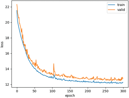
The loss curves obtained from the training and validation sets show the stability of our model. From Fig. 2, we can observe that the training and validation losses decreased to a point of stability and have a small gap between training and validation throughout the epochs. As the deep learning algorithms progress (that is, as they reach a high epoch value), the loss decreases and is stabilized, indicating that our neural network is learning in the right direction. This phenomenon also shows the optimal fit of our model to the data set.

Fig. 2. Loss curve during model training and validation.

Table VI summarizes the classification accuracy of the test set in this study. It is noticeable that the prediction accuracy result from the test data set is above 90%. The results indicate that the classification in this model has high predictive power. In sum, the results suggest that detecting a country’s proliferation behavior using deep learning algorithms may be less tentative and more viable than other existing methods.

TABLE VI Results of the MLP Model

Result	MLP
Validation accuracy (%)	98.037
Validation loss score	12.512
Test accuracy (%)	97.821

One limitation of our approach is inherent in the history of proliferation, and the relative rarity of the exploration, pursuit, and certainty of acquisition of nuclear weapons. Currently, there are 31 countries that have at least explored the development of nuclear programs in our data set. This low rate of nuclear proliferation impedes fitting the model to the data set due to the class imbalanced distribution. That is, if the data set primarily consists of the No Interest class, the importance of the Pursue or Acquire classes could be considered relatively low. Deep learning algorithms can show poor predictive performance of each classification level when faced by these skewed class distributions, despite a high accuracy score.

Therefore, we used additional metrics: precision, recall, and the F-1 score of each level of the classification results using a confusion matrix.^b Of all the observations where the target is in a specific level, the recall value tells us what fraction of all certain level samples were correctly predicted. Meanwhile, of all the observations where the prediction is at a specific level, the precision value tells us what fraction of predictions in each class were actually correct. The F-1 score is the harmonic mean of precision and recall. F-1 scores can be useful in evaluating the prediction capability of each classification level when using an imbalanced data set.

Table VII represents the precision, recall, and F-1 values from the confusion matrix of the test result depicted in the Appendix. The F-1 value of the Explore level was the lowest among all the other levels (except the Acquire level; about 74% in Table VII). This suggests that it is difficult to accurately identify the boundary between the No Interest and Explore levels of a country. This is unsurprising; the difference between a country having no interest in nuclear weapons and a country exploring nuclear weapons is a matter of interpretation, including by those coding the data sets. In the initial stages, a country developing a civil nuclear energy sector or a nuclear research capacity without any weapons intentions would likely look similar in terms of industrial capacity, knowledge networks, and even certain aspects of the nuclear fuel cycle to a country developing a nuclear energy or research capacity with a future interest in nuclear weapons. Moreover, given nuclear latency, the leaders of the country moving from No Interest to Explore may not themselves know when the transition occurs. With that said, the results still confirm that the deep learning algorithm using cross-country time data sets could be useful to predict a country’s active nuclear program (Pursue) initiation.

TABLE VII Precision, Recall, and F-1 Score of the Test Set

	Level	Score
Precision	No Interest	0.991
	Explore	0.840
	Pursue	0.692
	Acquire	0
Recall	No Interest	0.992
	Explore	0.656
	Pursue	0.947
	Acquire	0
F-1 Score	No Interest	0.991
	Explore	0.737
	Pursue	0.800
	Acquire	0

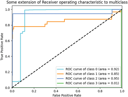
Next, we present the receiver operating characteristics (ROC) curve for the test data set results (see Fig. 3). The ROC curve plots recall against specificity (that is, the ratio of correct negative predictions to the total number of negative targets). A model with high predictability will have high recall and specificity simultaneously, which causes a ROC curve to move toward the top left corner of the plot. The area under the ROC curve (AUC) values (ranging in value from 0 to 1) of each level were mostly over 0.8, which implies that our MLP model is robust. However, similar to the results of the F-1 values in Table VII, we can see that the AUC value of the Explore class (0.85) in Fig. 3 implies that imbalanced distribution will result in a lower predictive power in differentiating between the No interest and Explore classes.

Fig. 3. ROC curve of the test results.

IV. DISCUSSION

IV.A. Cross Validation

In this study, we used a total of six layers of MLP to classify the proliferation risk levels. To examine how much better this six-layer MLP model fits the data than other machine learning algorithms, we used the stratified k-fold cross-validation method to train and test the different MLP and machine learning models. Cross validation is a resampling method using multiple training and validation sets, thereby examining the predictive power of different models. Therefore, scholars use cross-validation methods to compare and select a model best suited for the data set.

In a stratified five-fold cross validation, we first divided the data randomly into five subsamples by stratified random sampling. Then, we ran each deep learning model onto the training set (four subsamples) and measured the accuracy of the testing set (one subsample). Since we divided into five subsamples, this process was repeated five times for each epoch. That is, each stratified five-fold subset was played as the testing set. Then the average accuracy across all five trials was computed for each model to represent the predictive power.

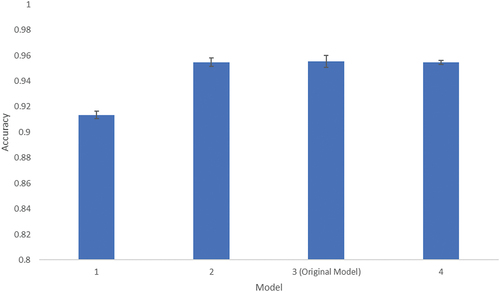
We set four different MLP models in this analysis, including the original model. We set the specifications of the models in the method section in this cross-validation analysis (i.e., batch number, epoch number). We used the same data set in this analysis. The model specifications are summarized in Table VIII.

TABLE VIII MLP Model Specification in the Five-Fold Cross-Validation Analysis

Specification	Model 1	Model 2	Model 3 (Original Model)	Model 4
Number of layers	2	4	6	8
Perceptrons for each layer	(41, 4)	(41, 20, 10, 4)	(41, 28, 20, 12, 8, 4)	(41, 36, 32, 24, 16, 12, 8, 4)

In summary, the six-layer MLP model showed the best prediction performance among the other MLP models. When we looked at the results depicted in model 1, which consisted of only two layers, the lowest prediction capability was demonstrated (0.9135). Model 4 (0.9545), with eight layers, also had a slightly lower prediction capability than model 3 (0.9553) (the original model in this study with six layers) (Fig. 4). This reflects that adding more layers to the MLP model in a certain level could lead to overfitting problems, and suggests that our original model is the preferred model.

Fig. 4. Stratified five-fold cross-validation results of different MLP models.

Next, we tested the predictive accuracy of the six-layer MLP model with other classification machine learning algorithms: multinomial logistic regression, support vector classifier (SVC), k-nearest neighbors (kNN) algorithms, and Naïve-Bayes (NB) classifiers. We examined the predictive accuracy using the stratified five-fold cross validation with the same data set. Table IX summarizes the comparison average, maximum, and minimum classification accuracies of the proliferation risk level classification among the machine learning algorithms.

TABLE IX Stratified Five-Fold Cross-Validation Results of Different Machine Learning Algorithms

Machine Learning Model	Average Accuracy (%)	Maximum Accuracy (%)	Minimum Accuracy (%)
MLP (six-layer)	95.534	96.841	94.009
Multinomial logistic regression	87.400	93.207	78.105
SVC	75.648	80.501	71.756
kNN	93.198	93.899	92.585
NB (Bernoulli)	78.769	85.605	58.824

From the results, it is evident that the MLP classifiers outperformed the other classifiers. The average classification accuracy of MLP was the highest among all the other machine learning models. The same tendencies were obtained with the minimum and maximum accuracy results. It is noticeable that the MLP accuracy was about 8 percentage points higher than the typical multinomial logistic regression models used by previous scholars. This again supports our contention that a deep learning algorithm shows a higher predictive power of nuclear proliferation risk than other classification models.

IV.B. Predicting North Korea and Iran Proliferation Levels Using MLP

The limitation of our data set construction is that it has a pooled–time series structure. That is, if country-year observations are chosen randomly, then the training data could contain, for example, North Korea 1981 and North Korea 1983. Using this training data set to predict North 1982 in the test data set would not be a demanding task, as the observations change very slowly from year to year within a given country’s time series. While this data set construction approach can impede predicting the real world, our preliminary MLP model showed a high accuracy of predictability.

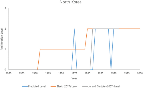
As a means of validating the results with real-world cases, we also used deep learning algorithms to project the proliferation decisions of North Korea and Iran, the two countries of greatest proliferation concern in recent years, against the historical records from those countries (Table II). We first trained the MLP model using data sets that successively excluded each country (North Korea and Iran). We then selected the best model from the validation process. The training and validation data sets were separated with stratified sampling methods, 80% and 20%, respectively. Using the model that best suits the validation set, we projected the results on the test set (in this case, North Korea, and Iran, respectively). The projection results using the trained model were then compared with historical proliferation events with proliferation timelines suggested by Bleek^[19] and Jo and Gartzke.^[5]

In the case of North Korea, similar trends in the projection results were observed in the Pursue level compared to Bleek and Jo and Gartzke (who differed from each other in terms of the dates for exploration and pursuit of nuclear weapons, in part due to the opacity of North Korea’s program) (see Fig. 5). For the Explore decision, however, the model did not predict the early signs of proliferation activities, while the actual proliferation Explore decision took place from the 1960s to the 1970s. This is in line with the previous results, which suggested that imbalanced distribution will decrease our ability to differentiate between the No Interest and Explore classes. Last, the one peak in 1975 in our projection results is when North Korea requested that China assist with its nuclear weapons programs.^[19]

Fig. 5. Projection of North Korea.

The same process was conducted in the Iran case. In the case of Iran, the projection results showed less similar trends in the Pursue level with Bleek^[19] than the North Korea case (see Fig. 6). However, the results show that the deep learning model captured well the Explore and Pursue proliferation periods coded by Bleek.^[19] Moreover, the projection results of the Pursue level were similar to the proliferation timeline of Jo and Gartzke.^[5] For example, Jo and Gartzke^[5] coded Iran’s pursuit of nuclear weapon programs as starting in 1974, ending in 1979 (with the Iranian revolution), and starting again in 1984, which is in line with our projection results. However, Iran was coded as exploring nuclear weapons from 1984 to 1988 in Bleek’s data set.^[19] The year 1984 is when Iran reinvigorated covert work on uranium conversion, fuel fabrication, and enrichment, without declaring its activities to the International Atomic Energy Agency (IAEA).^[19]

Fig. 6. Projection of Iran.

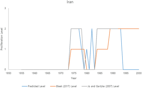
The differences in the results are likely due to differing understandings of a nuclear weapons program by the authors. These differences highlight the difficulty of interpreting a country’s intentions for activities that are, after all, quite often secret and designed to be plausibly deniable. While Jo and Gartzke^[5] only coded whether a state had an active nuclear weapons development program in a given year and did not code whether a state was interested in a nuclear program, this study indicates that deep learning models can predict a country’s active nuclear program, although the coded data may have uncertainty.

V. CONCLUSION

This paper examined the extent of prediction capability by integrating identified variables in the existing literature to explain nuclear proliferation. We presented a deep learning framework, specifically MLP, and applied it to the historical proliferation timelines of over 100 countries. We used 41 variables that were found to be significant determinants in previous studies for explaining the country’s proliferation. To classify the country’s historical nuclear program progression, 60%, 20%, and 20% of the collected data set were used as a training set, validation set, and testing set, respectively. We also employed cross validation to compare with machine learning tools and different MLP layers.

By employing a deep learning algorithm, this study improved the modeling-based prediction capability relative to previous econometrics-based studies. Previous studies pointed out that the determinants of proliferation identified as significant do not provide an improved ability to predict proliferation levels, although they were generally able to explain proliferation with varying degrees of success. However, the classification model developed in this study, which integrates the identified proliferation determinants from previous studies, distinguishes the levels of proliferation activity of a country with over 90% accuracy compared with historical data, suggesting that existing proliferation determinants are appropriate but may benefit from the application of a deep learning model. Compared to previous models, the deep learning model showed outstanding and robust prediction accuracy. In terms of using MLP models to project the proliferation-related behavior of a country, the additional use of the tacit knowledge and nuclear fuel cycle capability variables in the proliferation-assessing models could be considered to effectively predict a country’s nuclear proliferation–related behavior.

The classification model provides positive evidence to strengthen nuclear security by moving beyond the existing limitations that previous studies faced with proliferation prediction. This study highlights that the nonparametric prediction method made the best classification results compared with previous statistical prediction analyses. Although this deep learning method cannot explain the causality of proliferation causes and consequences, this study sheds light on the possibility of developing a tool to predict and prevent future nuclear programs of aspiring/civilian nuclear countries.

Disclosure Statement

No potential conflict of interest was reported by the authors.

Additional information

Funding

Yim acknowledges the financial support from the National Research Foundation of Korea (NRF-2022M2C7A1A02063817).

Notes

^a Acquire level observations of North Korea are not included in this data set because North Korea conducted its first nuclear weapons test after 2000.

^b The confusion matrix gives the detailed results of what the MLP model predicted on the test set. The confusion matrix of our test set prediction results is shown in the Appendix.

APPENDIX

CONFUSION MATRIX

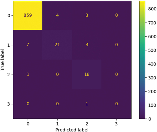
Figure A.1 presents the confusion matrix of the test set prediction results. In a confusion matrix, the true output level of proliferation is on one axis, and the predicted level of proliferation is on the other. It shows the comparison between the true label and the predicted label in the test set. The number of correct classifications is on the diagonal of each confusion matrix.

Fig. A.1. Confusion matrix of the test results.

References

- R. S. KEMP, “The Nonproliferation Emperor Has No Clothes: The Gas Centrifuge, Supply-Side Controls, and the Future of Nuclear Proliferation,” Int. Secur., 38, 4, 39 (2014); http://dx.doi.org/10.1162/ISEC_a_00159.
- S. M. MEYER, The Dynamics of Nuclear Proliferation, University of Chicago Press (1986).
- S. D. SAGAN, “Why Do States Build Nuclear Weapons? Three Models in Search of a Bomb,” Int. Secur., 21, 3, 54 (1996); http://dx.doi.org/10.2307/2539273.
- S. SINGH and C. R. WAY, “The Correlates of Nuclear Proliferation: A Quantitative Test,” J. Conflict Resolut., 48, 6, 859 (2004); http://dx.doi.org/10.1177/0022002704269655.
- D. JO and E. GARTZKE, “Determinants of Nuclear Weapons Proliferation,” J. Conflict Resolut., 51, 1, 167 (2007); http://dx.doi.org/10.1177/0022002706296158.
- M. FUHRMANN, “Spreading Temptation: Proliferation and Peaceful Nuclear Cooperation Agreements,” Int. Secur., 34, 7, 7 (2009); http://dx.doi.org/10.7591/cornell/9780801450907.003.0008.
- M. KROENIG, “Importing the Bomb: Sensitive Nuclear Assistance and Nuclear Proliferation,” J. Conflict Resolut., 53, 2, 161 (2009); http://dx.doi.org/10.1177/0022002708330287.
- J. LI, M. S. YIM, and D. N. MCNELIS, “Model-Based Calculations of the Probability of a Country’s Nuclear Proliferation Decisions,” Prog. Nucl. Energy, 52, 8, 789 (2010); http://dx.doi.org/10.1016/j.pnucene.2010.07.001.
- R. L. BROWN and J. M. KAPLOW, “Talking Peace, Making Weapons: IAEA Technical Cooperation and Nuclear Proliferation,” J. Conflict Resolut., 58, 3, 402 (2014); http://dx.doi.org/10.1177/0022002713509052.
- M. S. BELL, “Examining Explanations for Nuclear Proliferation,” Int. Stud. Q., 60, 3, 520 (2016); http://dx.doi.org/10.1093/isq/sqv007.
- M. S. YIM and J. LI, “Examining Relationship Between Nuclear Proliferation and Civilian Nuclear Power Development,” Prog. Nucl. Energy, 66, 108 (2013); http://dx.doi.org/10.1016/j.pnucene.2013.03.005.
- M. FUHRMANN, Atomic Assistance: How “Atoms for Peace” Programs Cause Nuclear Insecurity, Cornell University Press (2012).
- J. V. HASTINGS, A. N. STULBERG, and P. BAXTER, “Technology, Materials, and Knowledge Transfer in Nuclear Proliferation Networks: Findings and Implications,” University of Sydney (2015).
- P. BAXTER et al., “Mapping the Development of North Korea’s Domestic Nuclear Research Networks,” Rev. Policy Res., 39, 2, 219 (2022); http://dx.doi.org/10.1111/ropr.12462.
- J. E. C. HYMANS, Achieving Nuclear Ambitions: Scientists, Politicians, and Proliferation, Cambridge University Press (2012).
- A. H. MONTGOMERY, “Stop Helping Me: When Nuclear Assistance Impedes Nuclear Programs,” in The Nuclear Renaissance and International Security, A. STULBERG and M. FUHRMANN Eds., pp. 177–202, Stanford University Press (2013).
- P. M. BAXTER, “Nuclear Communities: Epistemic Community Structure and Nuclear Proliferation Latency,” Georgia Institute of Technology (2021).
- J. M. KAPLOW and E. GARTZKE, “Predicting Proliferation: High Reliability Forecasting Models of Nuclear Proliferation as a Policy and Analytical Aid,” Center on Contemporary Conflict (CCC) Project on Advanced Systems and Concepts for Countering Weapons of Mass Destruction (PASCC). Reports (2016).
- P. C. BLEEK, “When Did (and Didn’t) States Proliferate? Chronicling the Spread of Nuclear Weapons,” Belfer Center for Science and International Affairs (2017).
- J. D. SINGER, “Reconstructing the Correlates of War Dataset on Material Capabilities of States, 1816–1985,” Int. Interact., 14, 2, 115 (1988); http://dx.doi.org/10.1080/03050628808434695.
- M. FUHRMANN and B. TKACH, “Almost Nuclear: Introducing the Nuclear Latency Dataset,” Confl. Manag. Peace Sci., 32, 4, 443 (2015); http://dx.doi.org/10.1177/0738894214559672.
- M. KROENIG, “Exporting the Bomb: Why States Provide Sensitive Nuclear Assistance,” Am. Polit. Sci. Rev., 103, 1, 113 (2009); http://dx.doi.org/10.1017/S0003055409090017.
- “List of Member States,” International Atomic Energy Agency; https://www.iaea.org/about/governance/list-of-member-states ( current as of Mar. 20, 2020).
- P. KIM, J. KIM, and M. YIM, “Assessing Proliferation Uncertainty in Civilian Nuclear Cooperation Under New Power Dynamics of the International Nuclear Trade,” Energy Policy., 163, 112852 (Feb. 2022); http://dx.doi.org/10.1016/j.enpol.2022.112852.
- S. RAVICHANDIRAN, Hands-on Deep Learning Algorithms with Python: Master Deep Learning Algorithms with Extensive Math by Implementing Them Using Tensorflow, Packt Publishing Ltd (2019).
- A. GÉRON, Hands-on Machine Learning with Scikit-Learn, Keras, and TensorFlow: Concepts, Tools, and Techniques to Build Intelligent Systems, O’Reilly Media (2019).
- S. IOFFE and C. SZEGEDY, “Batch Normalization: Accelerating Deep Network Training by Reducing Internal Covariate Shift,” Proc. Int. Conf. on Machine Learning, p. 448, Proceedings of Machine Learning Research (2015).