A New Proof of the Asymptotic Diffusion Limit of the S_N Neutron Transport Equation

Abstract

It has been well known that the analytic neutron transport solution tends to the analytic solution of a diffusion problem for optically thick systems with small absorption and source. The standard technique for proving the asymptotic diffusion limit is constructing an asymptotic power series of the neutron angular flux in small positive parameter $\epsilon$, which is the ratio of a typical mean free path of a particle to a typical dimension of the problem domain. In this paper, first, we provide an analysis of the asymptotic properties of the S_N transport eigenvalues. Then, we show that the analytical S_N transport solution satisfies the diffusion equation in the asymptotic diffusion limit based on a recently obtained closed-form analytical solution to the one-dimensional monoenergetic S_N neutron transport equation. The boundary conditions for the diffusion equation are discussed.

Keywords:

• S_N transport equation
• transport eigenvalues
• analytical solution
• asymptotic diffusion limit

I. INTRODUCTION

The asymptotic analysis methodology originally developed by Larsen and others has proved to be a powerful technique to study transport problems^1–5 and analyze numerical methods.^6–9 The essential idea of the asymptotic analysis method is to assume a solution (the flux) that depends on a small parameter $\epsilon$ by a simple asymptotic expansion: $\psi =\sum _{i=0}^{\mathrm{\infty }}{\psi }^{\left(i\right)}{\epsilon }^i$. Larsen et al. used the asymptotic analysis to show the transition from analytic transport to analytic diffusion for the S_N transport equation.⁶ Most recently, to study the asymptotical properties of numerical schemes for the S_N transport equation, we proposed a different asymptotic analysis method that is based on the scaled Taylor expansion.¹⁰

In this paper, we present a direct proof to show that the analytical solution of the S_N transport equation satisfies the diffusion equation in the asymptotic diffusion limit. To facilitate the discussion, we first present a new closed-form analytical expression of the solution to the monoenergetic S_N transport equation in slab geometry,¹¹ which is essential for the proof. Then, the proof will follow naturally as the asymptotic properties of the S_N transport eigenvalues.

It should be noted that a number of analytical solutions and their numerical implementations have been proposed for the one-dimensional S_N transport equation.^12–17 Our solution is essentially similar to those matrix exponential formulations.^14,15,18 A comprehensive review of the matrix-exponential formalism in radiative transfer can be found in the literature.¹⁹ The S_N transport equation is decoupled by eigen decomposition. In general, we can consider the eigenvalues and eigenvectors as known since they can be easily obtained using a modern software with arbitrarily high precision.²⁰ The decoupled set of linear first-order ordinary differential equations is solved analytically in matrix form based on the classical method of characteristics. One can find the detailed derivation in Ref. 11. Here, we briefly summarize the solution as follows.

The steady monoenergetic S_N equation in slab geometry assuming isotropic scattering and constant neutron source is written as

(1) $\mu \frac{d}{dx}\mathbf{\Psi }+{\mathrm{\Sigma }}_t\mathbf{\Psi }=\frac{{\mathrm{\Sigma }}_s}{2}\mathbf{W}\mathbf{\Psi }+\frac{Q}{2}\mathbf{1},$(1)

where

(2) $\begin{array}{r}\mathbf{\Psi }={\left[\begin{array}{cccc}{\psi }_1& {\psi }_2& \hspace{0.17em}\dots \hspace{0.17em}& {\psi }_N\end{array}\right]}^{\mathit{T}}=\text{angular flux vector}\end{array}$(2)

(3) $\mu ={\left[\begin{array}{cc}\mu & \hspace{0.17em}\\ \hspace{0.17em}& -\mu \end{array}\right]}_{N\times N}=\text{rm{cosine of the neutron direction relative to}}x-\mathrm{a}\mathrm{x}\mathrm{i}\mathrm{s},$(3)

in which

(4) $\mu =\mathrm{d}\mathrm{i}\mathrm{a}\mathrm{g}\left({\mu }_n\right)>0,n=1,\dots ,\frac{N}{2}$(4)

(5) $\mathbf{W}={\left[\begin{array}{cc}\mathbf{w}& \mathbf{w}\\ \mathbf{w}& \mathbf{w}\end{array}\right]}_{N\times N}\text{rm{ = quadrature weights}},$(5)

in which

(6) $\mathbf{w}={\left[\begin{array}{cccc}{w}_1& w_2& \dots & w_{\frac{N}{2}}\\ w_1& w_2& \dots & w_{\frac{N}{2}}\\ ⋮& ⋮& \ddots & w_{\frac{N}{2}}\\ w_1& w_2& \dots & w_{\frac{N}{2}}\end{array}\right]}_{\frac{N}{2}\times \frac{N}{2}}$(6)

(7) $\sum _{n=1}^{\frac{N}{2}}{w}_n=1$(7)

(8) $\mathbf{1}={\left[\begin{array}{cccc}1& 1& \hspace{0.17em}\dots \hspace{0.17em}& 1\end{array}\right]}^{\mathit{T}}$(8)

${\mathrm{\Sigma }}_t=$ total macroscopic cross section

${\mathrm{\Sigma }}_s=$ macroscopic scattering cross section

$Q=$ constant neutron source.

Equation (1)(1) $\mu \frac{d}{dx}\mathbf{\Psi }+{\mathrm{\Sigma }}_t\mathbf{\Psi }=\frac{{\mathrm{\Sigma }}_s}{2}\mathbf{W}\mathbf{\Psi }+\frac{Q}{2}\mathbf{1},$(1) is a system of coupled first-order differential equations. Matrices $\mu$ and $\mathbf{W}$ contain the nodes and weights of a symmetric quadrature set (e.g., Gauss-Legendre quadrature).

We can write Eq. (1)(1) $\mu \frac{d}{dx}\mathbf{\Psi }+{\mathrm{\Sigma }}_t\mathbf{\Psi }=\frac{{\mathrm{\Sigma }}_s}{2}\mathbf{W}\mathbf{\Psi }+\frac{Q}{2}\mathbf{1},$(1) as

(9) $\frac{d}{dx}\mathbf{\Psi }+{\mathrm{\Sigma }}_t{\mu }^{-1}\left(\mathbf{I}-\frac{c}{2}\mathbf{W}\right)\mathbf{\Psi }=\mathbf{q},$(9)

where

(10) $c=\frac{{\mathrm{\Sigma }}_s}{{\mathrm{\Sigma }}_t}=\text{rm{scattering ratio}}$(10)

and

(11) $\mathbf{q}=\frac{Q}{2}{\mu }^{-1}\mathbf{1}.$(11)

The transport matrix ${\mathrm{\Sigma }}_t{\mu }^{-1}\left(\mathbf{I}-\frac{c}{2}\mathbf{W}\right)$ is diagonalizable, and we have

(12) ${\mathrm{\Sigma }}_t{\mu }^{-1}\left(\mathbf{I}-\frac{c}{2}\mathbf{W}\right)=\mathbf{R}\mathbf{\Lambda }{\mathbf{R}}^{-1},$(12)

where $\mathbf{\Lambda }$ is the diagonal matrix with the eigenvalues of the matrix ${\mathrm{\Sigma }}_t{\mu }^{-1}\left(\mathbf{I}-\frac{c}{2}\mathbf{W}\right)$ and $\mathbf{R}$ is the matrix with the columns consisting of eigenvectors. We can find $\mathbf{R}$ and $\mathbf{\Lambda }$ through eigen decomposition. If $c=0,$ the eigenvalues and eigenvectors are simply ${\mathrm{\Sigma }}_t{\mu }^{-1}$ and the identity matrix I, respectively.

We write $\mathbf{\Lambda }$ as

(13) $\mathbf{\Lambda }=\left[\begin{array}{cc}{\mathbf{\Lambda }}_{+}& \hspace{0.17em}\\ \hspace{0.17em}& {\mathbf{\Lambda }}_{-}\end{array}\right],$(13)

where

(14a) ${\mathbf{\Lambda }}_{+}=\mathrm{d}\mathrm{i}\mathrm{a}\mathrm{g}\left({\lambda }_n\right),n=1,\dots \frac{N}{2}$(14a)

and

(14b) ${\mathbf{\Lambda }}_{-}=\mathrm{d}\mathrm{i}\mathrm{a}\mathrm{g}\left({\lambda }_n\right),n=\frac{N}{2},\dots N.$(14b)

We will show in Sec. II that all the eigenvalues are real and that they occur in positive-negative pairs as

(15a) ${\mathbf{\Lambda }}_{+}>0$(15a)

and

(15b) ${\mathbf{\Lambda }}_{-}=-{\mathbf{\Lambda }}_{+}<0.$(15b)

The detailed solution process can be found in Ref. 11. We just give the final analytical solution for the angular flux as just

$\begin{array}{rl}\mathbf{\Psi }=& \frac{Q}{2}\frac{1}{{\mathrm{\Sigma }}_t\left(1-c\right)}\mathbf{1}-\mathbf{R}\left[\begin{array}{cc}{e}^{-x{\mathbf{\Lambda }}_{+}}& \hspace{0.17em}\\ \hspace{0.17em}& e^{\left(L-x\right){\mathbf{\Lambda }}_{-}}\end{array}\right]\\ & {\mathbf{R}}^{-1}\left(\frac{Q}{2}\frac{1}{{\mathrm{\Sigma }}_t\left(1-c\right)}\mathbf{1}-\mathbf{R}\left[\begin{array}{c}{\mathbb{Y}}_{+}^0\\ {\mathbb{Y}}_{-}^L\end{array}\right]\right).(16)\end{array}$

Then, the scalar flux can be calculated as

$\begin{array}{rl}\varphi =& {\mathbb{W}}^{\mathit{T}}\mathbf{\Psi }\\ =& \frac{Q}{{\mathrm{\Sigma }}_t\left(1-c\right)}-{\mathbb{W}}^T\mathbf{R}\left[\begin{array}{cc}{e}^{-x{\mathbf{\Lambda }}_{+}}& \hspace{0.17em}\\ \hspace{0.17em}& e^{\left(L-x\right){\mathbf{\Lambda }}_{-}}\end{array}\right]\\ & {\mathbf{R}}^{-1}\left(\frac{Q}{2}\frac{1}{{\mathrm{\Sigma }}_t\left(1-c\right)}\mathbf{1}-\mathbf{R}\left[\begin{array}{c}{\mathbb{Y}}_{+}^0\\ {\mathbb{Y}}_{-}^L\end{array}\right]\right),(17)\end{array}$

where

(18a) $\mathbb{W}={\left[\begin{array}{cccccccc}{w}_1& w_2& \cdots & w_{\frac{N}{2}}& w_1& w_2& \hspace{0.17em}\dots \hspace{0.17em}& w_{\frac{N}{2}}\end{array}\right]}^{\mathit{T}}$(18a)

(18b) $\begin{array}{rl}\left[\begin{array}{c}{\mathbb{Y}}_{+}^0\\ {\mathbb{Y}}_{-}^{\mathrm{L}}\end{array}\right]=& {\left[\begin{array}{cc}{\mathbf{R}}_{11}& {\mathbf{R}}_{12}{e}^{L{\mathbf{\Lambda }}_{-}}\\ {\mathbf{R}}_{21}{e}^{-L{\mathbf{\Lambda }}_{+}}& {\mathbf{R}}_{22}\end{array}\right]}^{-1}\left\{\left[\begin{array}{c}{\mathbf{\Psi }}_{+}^0\\ {\mathbf{\Psi }}_{-}^{\mathbf{L}}\end{array}\right]\right.\\ & -\left[\begin{array}{cc}\hspace{0.17em}& {\mathbf{R}}_{12}\left(\mathbf{I}-e^{L{\mathbf{\Lambda }}_{-}}\right)\\ {\mathbf{R}}_{21}\left(\mathbf{I}-e^{-L{\mathbf{\Lambda }}_{+}}\right)& \hspace{0.17em}\end{array}\right]\\ & -\left.\left[\begin{array}{c}{\mathbf{\Lambda }}_{+}^{-1}{\mathbf{b}}_{+}\\ {\mathbf{\Lambda }}_{-}^{-1}{\mathbf{b}}_{-}\end{array}\right]\right\}\end{array}$(18b)

(18c) $\mathbf{b}=\left[\begin{array}{c}{\mathbf{b}}_{+}\\ {\mathbf{b}}_{-}\end{array}\right]={\mathbf{R}}^{-1}\mathbf{q}$(18c)

(18d) ${\mathbf{\Psi }}_{+}^0\text{rm{ = incoming angular flux at}}x=0$(18d)

(18e) ${\mathbf{\Psi }}_{-}^{\mathbf{L}}\text{rm{ = incoming angular flux at}}x=L.$(18e)

Remark: We derived the general solution in a straightforward way by combining the left and right incoming angular flux vectors into a single vector as shown in Eq. (18b)(18b) $\begin{array}{rl}\left[\begin{array}{c}{\mathbb{Y}}_{+}^0\\ {\mathbb{Y}}_{-}^{\mathrm{L}}\end{array}\right]=& {\left[\begin{array}{cc}{\mathbf{R}}_{11}& {\mathbf{R}}_{12}{e}^{L{\mathbf{\Lambda }}_{-}}\\ {\mathbf{R}}_{21}{e}^{-L{\mathbf{\Lambda }}_{+}}& {\mathbf{R}}_{22}\end{array}\right]}^{-1}\left\{\left[\begin{array}{c}{\mathbf{\Psi }}_{+}^0\\ {\mathbf{\Psi }}_{-}^{\mathbf{L}}\end{array}\right]\right.\\ & -\left[\begin{array}{cc}\hspace{0.17em}& {\mathbf{R}}_{12}\left(\mathbf{I}-e^{L{\mathbf{\Lambda }}_{-}}\right)\\ {\mathbf{R}}_{21}\left(\mathbf{I}-e^{-L{\mathbf{\Lambda }}_{+}}\right)& \hspace{0.17em}\end{array}\right]\\ & -\left.\left[\begin{array}{c}{\mathbf{\Lambda }}_{+}^{-1}{\mathbf{b}}_{+}\\ {\mathbf{\Lambda }}_{-}^{-1}{\mathbf{b}}_{-}\end{array}\right]\right\}\end{array}$(18b) . The final solution is an explicit closed-form expression of eigen exponential functions, and it applies for $c\in \left[0,1\right)$. When the scattering ratio $c$ is extremely close to 1, there will be a loss of precision in the solution. To achieve high-precision solutions, one needs to use software with multiprecision capability.²⁰ Our solution does not apply for the case of conservative scattering ($c=1$), in which the smallest eigenvalues vanish and the transport matrix becomes singular. However, in numerical computation we can always calculate the conservative case with our solution by limiting $c\to 1$. It is worth noting that an analytical approach to overcoming the difficulty with the conservative scattering is described by Efremenko et al.¹⁹ In addition, the analytical solution can be extended to solve the anisotropic scattering case and handle heterogeneous geometry without iterating on surface fluxes.²¹ It is also worth mentioning that a novel analytical nodal discrete ordinates method has recently been developed for solving the S_N equation in two-dimensional Cartesian geometry based on the analytical solution derived for slab geometry.²²

The remainder of this paper is organized as follows. In Sec. II, we present an analysis of the eigenvalues of the S_N equation in the asymptotic diffusion limit. Section III presents the proof of diffusion theory; i.e., the analytical solution of the S_N equation asymptotically satisfies the diffusion equation in the diffusion limit. The boundary conditions (BCs) for the diffusion equation are discussed. A numerical example is given in Sec. IV to compare the difference between the S_N transport solution and its diffusion counterpart. Finally, conclusions are given in Sec. V.

II. TRANSPORT EIGENVALUES IN THE ASYMPTOTIC LIMIT

Before we present the proof to show that the solution of the S_N transport equation tends to that of the diffusion equation in the asymptotic diffusion limit, we need to investigate the asymptotic properties of the eigenvalues of the transport matrix ${\mathrm{\Sigma }}_t{\mu }^{-1}\left(\mathbf{I}-\frac{c}{2}\mathbf{W}\right).$

Let

(19) $\mathbf{A}={\mathrm{\Sigma }}_t{\mu }^{-1}\left(\mathbf{I}-\frac{c}{2}\mathbf{W}\right).$(19)

The matrix $\mathbf{A}$ can be rewritten as

(20) $\begin{array}{rl}\mathbf{A}& =\left[\begin{array}{cc}{\mathrm{\Sigma }}_t{\mu }^{-1}& 0\\ 0& -{\mathrm{\Sigma }}_t{\mu }^{-1}\end{array}\right]\left[\begin{array}{cc}\mathbf{I}-\frac{c}{2}\mathbf{w}& -\frac{c}{2}\mathbf{w}\\ -\frac{c}{2}\mathbf{w}& \mathbf{I}-\frac{c}{2}\mathbf{w}\end{array}\right]\\ & =\left[\begin{array}{cc}{\mathrm{\Sigma }}_t{\mu }^{-1}-\frac{{\mathrm{\Sigma }}_{t}c}{2}{\mu }^{-1}\mathbf{w}& -\frac{{\mathrm{\Sigma }}_{t}c}{2}{\mu }^{-1}\mathbf{w}\\ \frac{{\mathrm{\Sigma }}_{t}c}{2}{\mu }^{-1}\mathbf{w}& -{\mathrm{\Sigma }}_t{\mu }^{-1}+\frac{{\mathrm{\Sigma }}_{t}c}{2}{\mu }^{-1}\mathbf{w}\end{array}\right],\end{array}$(20)

where $\mu$, $\mu$, $\mathbf{W}$, and $\mathbf{w}$ are defined in Eqs. (3)(3) $\mu ={\left[\begin{array}{cc}\mu & \hspace{0.17em}\\ \hspace{0.17em}& -\mu \end{array}\right]}_{N\times N}=\text{rm{cosine of the neutron direction relative to}}x-\mathrm{a}\mathrm{x}\mathrm{i}\mathrm{s},$(3) through (6(6) $\mathbf{w}={\left[\begin{array}{cccc}{w}_1& w_2& \dots & w_{\frac{N}{2}}\\ w_1& w_2& \dots & w_{\frac{N}{2}}\\ ⋮& ⋮& \ddots & w_{\frac{N}{2}}\\ w_1& w_2& \dots & w_{\frac{N}{2}}\end{array}\right]}_{\frac{N}{2}\times \frac{N}{2}}$(6) ), respectively. $\mathbf{I}$ is the identity matrix.

We can obtain the eigenvalues $\lambda$ through the following determinant of the matrix:

(21) $\begin{array}{rl}& det\left(\mathbf{A}-\lambda \mathbf{I}\right)\\ & =\left|\text{openup}4pt\begin{array}{cc}{\mathrm{\Sigma }}_t{\mu }^{-1}-\frac{{\mathrm{\Sigma }}_{t}c}{2}{\mu }^{-1}\mathbf{w}-\lambda \mathbf{I}& -\frac{{\mathrm{\Sigma }}_{t}c}{2}{\mu }^{-1}\mathbf{w}\\ \frac{{\mathrm{\Sigma }}_{t}c}{2}{\mu }^{-1}\mathbf{w}& -{\mathrm{\Sigma }}_t{\mu }^{-1}+\frac{{\mathrm{\Sigma }}_{t}c}{2}{\mu }^{-1}\mathbf{w}-\lambda \mathbf{I}\end{array}\right|=0.\end{array}$(21)

The value of the determinant does not change by adding the second row to the first row:

(22) $det\left(\mathbf{A}-\lambda \mathbf{I}\right)=\left|\text{openup}4pt\begin{array}{cc}{\mathrm{\Sigma }}_t{\mu }^{-1}-\lambda \mathbf{I}& -{\mathrm{\Sigma }}_t{\mu }^{-1}-\lambda \mathbf{I}\\ \frac{{\mathrm{\Sigma }}_{t}c}{2}{\mu }^{-1}\mathbf{w}& -{\mathrm{\Sigma }}_t{\mu }^{-1}+\frac{{\mathrm{\Sigma }}_{t}c}{2}{\mu }^{-1}\mathbf{w}-\lambda \mathbf{I}\end{array}\right|.$(22)

The value of the determinant does not change by adding the first column to the second column:

(23) $det\left(\mathbf{A}-\lambda \mathbf{I}\right)=\left|\text{openup}4pt\begin{array}{cc}{\mathrm{\Sigma }}_t{\mu }^{-1}-\lambda \mathbf{I}& -2\lambda \mathbf{I}\\ \frac{{\mathrm{\Sigma }}_{t}c}{2}{\mu }^{-1}\mathbf{w}& -{\mathrm{\Sigma }}_t{\mu }^{-1}+{\mathrm{\Sigma }}_{t}c{\mu }^{-1}\mathbf{w}-\lambda \mathbf{I}\end{array}\right|.$(23)

The value of the determinant does not change by multiplying the second column with $-\frac{1}{2}$ and then adding it to the first column:

(24) $det\left(\mathbf{A}-\lambda \mathbf{I}\right)=\left|\text{openup}4pt\begin{array}{cc}{\mathrm{\Sigma }}_t{\mu }^{-1}& -2\lambda \mathbf{I}\\ \frac{{\mathrm{\Sigma }}_t}{2}{\mu }^{-1}+\frac{\lambda }{2}\mathbf{I}& -{\mathrm{\Sigma }}_t{\mu }^{-1}+{\mathrm{\Sigma }}_{t}c{\mu }^{-1}\mathbf{w}-\lambda \mathbf{I}\end{array}\right|.$(24)

The value of the determinant does not change by adding the ($-\frac{1}{2}$) multiple of the first row to the second row, and then we obtain

(25) $det\left(\mathbf{A}-\lambda \mathbf{I}\right)=\left|\text{openup}4pt\begin{array}{cc}{\mathrm{\Sigma }}_t{\mu }^{-1}& -2\lambda \mathbf{I}\\ \frac{\lambda }{2}\mathbf{I}& -{\mathrm{\Sigma }}_t{\mu }^{-1}+{\mathrm{\Sigma }}_{t}c{\mu }^{-1}\mathbf{w}\end{array}\right|.$(25)

Since ${\mathrm{\Sigma }}_t{\mu }^{-1}$ is a nonsingular matrix, the determinant can be expressed as

(26) $\begin{array}{rl}& det\left(\mathbf{A}-\lambda \mathbf{I}\right)\\ & =det\left({\mathrm{\Sigma }}_t{\mu }^{-1}\right)det\left(-{\mathrm{\Sigma }}_t{\mu }^{-1}+{\mathrm{\Sigma }}_{t}c{\mu }^{-1}\mathbf{w}+{\lambda }^2{\mathrm{\Sigma }}_t^{-1}\mu \right)\\ & ={\left[det\left({\mathrm{\Sigma }}_t{\mu }^{-1}\right)\right]}^2\mathrm{d}\mathrm{e}\mathrm{t}\left[-\mathbf{I}+c\mathbf{w}+\frac{{\lambda }^2}{{\mathrm{\Sigma }}_t^2}{\mu }^2\right]=0.\end{array}$(26)

Since $det\left({\mathrm{\Sigma }}_t{\mu }^{-1}\right)\ne 0$, we obtain

(27) $\mathrm{d}\mathrm{e}\mathrm{t}\left[-\mathbf{I}+c\mathbf{w}+\frac{{\lambda }^2}{{\mathrm{\Sigma }}_t^2}{\mu }^2\right]=0.$(27)

Using the Sherman-Morrison formula,²³ we obtain

(28) $\begin{array}{rl}& \mathrm{d}\mathrm{e}\mathrm{t}\left[-\mathbf{I}+c\mathbf{w}+\frac{{\lambda }^2}{{\mathrm{\Sigma }}_t^2}{\mu }^2\right]=\mathrm{d}\mathrm{e}\mathrm{t}\left[\frac{{\lambda }^2}{{\mathrm{\Sigma }}_t^2}{\mu }^2-\mathbf{I}+c{\mathbf{1}}_{\frac{N}{2}\times 1}{\mathbf{w}}_{1\times \frac{N}{2}}\right]\\ & =\mathrm{d}\mathrm{e}\mathrm{t}\left(\frac{{\lambda }^2}{{\mathrm{\Sigma }}_t^2}{\mu }^2-\mathbf{I}\right)\cdot \left(1+c{\mathbf{w}}_{1\times \frac{N}{2}}{\left(\frac{{\lambda }^2}{{\mathrm{\Sigma }}_t^2}{\mu }^2-\mathbf{I}\right)}^{-1}{\mathbf{1}}_{\frac{N}{2}\times 1}\right)=0,\end{array}$(28)

where

(29) ${\mathbf{w}}_{1\times \frac{N}{2}}=\left[\begin{array}{cccc}{w}_1& w_2& \cdots & w_{N/2}\end{array}\right]$(29)

and

(30) ${\mathbf{1}}_{\frac{N}{2}\times 1}=\left[\begin{array}{c}1\\ 1\\ ⋮\\ 1\end{array}\right].$(30)

If $c=0$, which is the purely absorbing case, then we have

(31) $\mathrm{d}\mathrm{e}\mathrm{t}\left(\frac{{\lambda }^2}{{\mathrm{\Sigma }}_t^2}{\mu }^2-\mathbf{I}\right)=0,$(31)

and thus,

(32) ${\lambda }_i=\frac{{\mathrm{\Sigma }}_t}{{\mu }_i},i=1,\dots ,\frac{N}{2}.$(32)

Here, we are interested in the case of $c\ne 0$. Now that $\mathrm{d}\mathrm{e}\mathrm{t}\left(\frac{{\lambda }^2}{{\mathrm{\Sigma }}_t^2}{\mu }^2-\mathbf{I}\right)\ne 0$, we have

(33) $\left(1+c{\mathbf{w}}_{1\times \frac{N}{2}}{\left(\frac{{\lambda }^2}{{\mathrm{\Sigma }}_t^2}{\mu }^2-\mathbf{I}\right)}^{-1}{\mathbf{1}}_{\frac{N}{2}\times 1}\right)=0.$(33)

Then, we have

(34) $\begin{array}{r}-{\mathbf{w}}_{1\times \frac{N}{2}}{\left(\frac{{\lambda }^2}{{\mathrm{\Sigma }}_t^2}{\mu }^2-\mathbf{I}\right)}^{-1}{\mathbf{1}}_{\frac{N}{2}\times 1}=\sum _{i=1}^{N/2}\frac{w_i}{1-\frac{{\lambda }^2{\mu }_i^2}{{\mathrm{\Sigma }}_t^2}}=\frac{1}{c}\end{array}.$(34)

The characteristic equation, Eq. (34(34) $\begin{array}{r}-{\mathbf{w}}_{1\times \frac{N}{2}}{\left(\frac{{\lambda }^2}{{\mathrm{\Sigma }}_t^2}{\mu }^2-\mathbf{I}\right)}^{-1}{\mathbf{1}}_{\frac{N}{2}\times 1}=\sum _{i=1}^{N/2}\frac{w_i}{1-\frac{{\lambda }^2{\mu }_i^2}{{\mathrm{\Sigma }}_t^2}}=\frac{1}{c}\end{array}.$(34) ), implies that all eigenvalues $\lambda$ are real and occur in positive-negative pairs for the case of $c<1$. If the roots of $\lambda$ were imaginary numbers, then $1-\frac{{\lambda }^2{\mu }_i^2}{{\mathrm{\Sigma }}_t^2}>1$, and we would have $\sum _{i=1}^{N/2}\frac{w_i}{1-\frac{{\lambda }^2{\mu }_i^2}{{\mathrm{\Sigma }}_t^2}}<1$ since $\sum _{i=1}^{N/2}{w}_i=1$, which is contradictory with $\frac{1}{c}>1$. The eigenvalues degenerate to zero in the limit of $c=1$, and they become imaginary roots for $c>1$. Here, we assume a symmetric quadrature with weights $w_i>0$ and $\left|{\mu }_i\right|<1$ for our argument. It should be noted that Davison deduced the same result for the monoenergetic S_N transport equation with isotropic scattering by using a heuristic approach.²⁴ A general proof on the spectrum of the transport operator was given by Kuscer and Vidav.²⁵

If $\frac{{\lambda }^2{\mu }_i^2}{{\mathrm{\Sigma }}_t^2}<1$ (it is shown later that the condition is satisfied for the smallest eigenvalue in the asymptotic diffusion limit), the above summation term can be expanded in a series of polynomials of ${\mu }_i$:

(35) $\begin{array}{rl}& \frac{w_i}{1-\frac{{\lambda }^2{\mu }_i^2}{{\mathrm{\Sigma }}_t^2}}\\ =& w_i\left[1+\left(\frac{{\lambda }^2}{{\mathrm{\Sigma }}_t^2}\right){\mu }_i^2+{\left(\frac{{\lambda }^2}{{\mathrm{\Sigma }}_t^2}\right)}^2{\mu }_i^4+{\left(\frac{{\lambda }^2}{{\mathrm{\Sigma }}_t^2}\right)}^3{\mu }_i^6+\cdots \right].\end{array}$(35)

It is known that the weights $w_i$ and nodes ${\mu }_i$ of the Gauss-Legendre quadrature can allow the quadrature rule to integrate degree $2N-1$ polynomials exactly. Therefore, for $N$ sufficiently large, the summation in Eq. (34)(34) $\begin{array}{r}-{\mathbf{w}}_{1\times \frac{N}{2}}{\left(\frac{{\lambda }^2}{{\mathrm{\Sigma }}_t^2}{\mu }^2-\mathbf{I}\right)}^{-1}{\mathbf{1}}_{\frac{N}{2}\times 1}=\sum _{i=1}^{N/2}\frac{w_i}{1-\frac{{\lambda }^2{\mu }_i^2}{{\mathrm{\Sigma }}_t^2}}=\frac{1}{c}\end{array}.$(34) is almost exactly equal to the following integral:

(36) $\sum _{i=1}^{N/2}\frac{w_i}{1-\frac{{\lambda }^2{\mu }_i^2}{{\mathrm{\Sigma }}_t^2}}\approx \underset{0}{\overset{1}{\int }}\frac{1}{1-\frac{{\lambda }^2{\mu }^2}{{\mathrm{\Sigma }}_t^2}}d\mu .$(36)

Then, we have

(37) $\underset{0}{\overset{1}{\int }}\frac{1}{1-\frac{{\lambda }^2{\mu }^2}{{\mathrm{\Sigma }}_t^2}}d\mu =\frac{{tanh}^{-1}\frac{\lambda }{{\mathrm{\Sigma }}_t}}{\frac{\lambda }{{\mathrm{\Sigma }}_t}}=\frac{1}{c}.$(37)

It is interesting to note that we arrive at the same formula as derived for the integrodifferential transport equation based on the singular eigenfunction method (separation of variables).²⁶

Now, we introduce the following scaling of cross sections:

(38) ${\mathrm{\Sigma }}_t=\frac{{\mathrm{\Sigma }}_{t0}}{\epsilon }$(38)

and

(39) ${\mathrm{\Sigma }}_a=\epsilon {\mathrm{\Sigma }}_{a0},$(39)

which implies

(40) ${\mathrm{\Sigma }}_s={\mathrm{\Sigma }}_t-{\mathrm{\Sigma }}_a=\frac{{\mathrm{\Sigma }}_{t0}}{\epsilon }-\epsilon {\mathrm{\Sigma }}_{a0}$(40)

and

(41) $c=\frac{{\mathrm{\Sigma }}_s}{{\mathrm{\Sigma }}_t}=1-{\epsilon }^2\frac{{\mathrm{\Sigma }}_{a0}}{{\mathrm{\Sigma }}_{t0}},$(41)

where $\epsilon$ is a small positive parameter and ${\mathrm{\Sigma }}_{t0}$ and ${\mathrm{\Sigma }}_{a0}$ are constants.

Substituting the scaling Eqs. (38)(38) ${\mathrm{\Sigma }}_t=\frac{{\mathrm{\Sigma }}_{t0}}{\epsilon }$(38) and (41(41) $c=\frac{{\mathrm{\Sigma }}_s}{{\mathrm{\Sigma }}_t}=1-{\epsilon }^2\frac{{\mathrm{\Sigma }}_{a0}}{{\mathrm{\Sigma }}_{t0}},$(41) ) into Eq. (37)(37) $\underset{0}{\overset{1}{\int }}\frac{1}{1-\frac{{\lambda }^2{\mu }^2}{{\mathrm{\Sigma }}_t^2}}d\mu =\frac{{tanh}^{-1}\frac{\lambda }{{\mathrm{\Sigma }}_t}}{\frac{\lambda }{{\mathrm{\Sigma }}_t}}=\frac{1}{c}.$(37) and letting $\epsilon \to 0$, we can find the two roots for $\lambda$, which are denoted by ${\lambda }_1$:

(42) ${\lambda }_1\to \pm \sqrt{3{\mathrm{\Sigma }}_{t0}{\mathrm{\Sigma }}_{a0}}=\pm \sqrt{3{\mathrm{\Sigma }}_t{\mathrm{\Sigma }}_a}.$(42)

It shows that in the asymptotic diffusion limit, the absolute value of ${\lambda }_1$ tends to a constant, which corresponds to the inverse of the diffusion length in reactor physics. Now, we verify $\frac{{\lambda }_1^2{\mu }_i^2}{{\mathrm{\Sigma }}_t^2}<1$. Since ${\mu }_i\le 1$, we only need to have $\frac{{\lambda }_1^2}{{\mathrm{\Sigma }}_t^2}<1$. We have $\frac{{\lambda }_1^2}{{\mathrm{\Sigma }}_t^2}=\frac{3{\mathrm{\Sigma }}_{t0}{\mathrm{\Sigma }}_{a0}}{{\left({\mathrm{\Sigma }}_{t0}/\epsilon \right)}^2}=3{\epsilon }^2\frac{{\mathrm{\Sigma }}_{a0}}{{\mathrm{\Sigma }}_{t0}}\ll 1$, which goes to zero quickly as $\epsilon \to 0$.

Next, we investigate the properties of other eigenvalues in the asymptotic diffusion limit. Since ${\lambda }_1$ are the two eigenvalues of the transport matrix, they should satisfy Eq. (34)(34) $\begin{array}{r}-{\mathbf{w}}_{1\times \frac{N}{2}}{\left(\frac{{\lambda }^2}{{\mathrm{\Sigma }}_t^2}{\mu }^2-\mathbf{I}\right)}^{-1}{\mathbf{1}}_{\frac{N}{2}\times 1}=\sum _{i=1}^{N/2}\frac{w_i}{1-\frac{{\lambda }^2{\mu }_i^2}{{\mathrm{\Sigma }}_t^2}}=\frac{1}{c}\end{array}.$(34) as

(43) $\sum _{i=1}^{N/2}\frac{w_i}{1-\frac{{\lambda }_1^2{\mu }_i^2}{{\mathrm{\Sigma }}_t^2}}=\frac{1}{c}.$(43)

Subtracting Eq. (43)(43) $\sum _{i=1}^{N/2}\frac{w_i}{1-\frac{{\lambda }_1^2{\mu }_i^2}{{\mathrm{\Sigma }}_t^2}}=\frac{1}{c}.$(43) from Eq. (34(34) $\begin{array}{r}-{\mathbf{w}}_{1\times \frac{N}{2}}{\left(\frac{{\lambda }^2}{{\mathrm{\Sigma }}_t^2}{\mu }^2-\mathbf{I}\right)}^{-1}{\mathbf{1}}_{\frac{N}{2}\times 1}=\sum _{i=1}^{N/2}\frac{w_i}{1-\frac{{\lambda }^2{\mu }_i^2}{{\mathrm{\Sigma }}_t^2}}=\frac{1}{c}\end{array}.$(34) ), we obtain

(44) $\sum _{i=1}^{N/2}\left(\frac{w_i}{1-\frac{{\lambda }^2{\mu }_i^2}{{\mathrm{\Sigma }}_t^2}}-\frac{w_i}{1-\frac{{\lambda }_1^2{\mu }_i^2}{{\mathrm{\Sigma }}_t^2}}\right)=\sum _{i=1}^{N/2}\frac{w_i{\mu }_i^2\left({\lambda }^2-{\lambda }_1^2\right)}{\left(1-\frac{{\lambda }^2{\mu }_i^2}{{\mathrm{\Sigma }}_t^2}\right)\left(1-\frac{{\lambda }_1^2{\mu }_i^2}{{\mathrm{\Sigma }}_t^2}\right)}=0.$(44)

Since $\left({\lambda }^2-{\lambda }_1^2\right)\ne 0$, we have

(45) $\sum _{i=1}^{N/2}\frac{w_i{\mu }_i^2}{\left(1-\frac{{\lambda }^2{\mu }_i^2}{{\mathrm{\Sigma }}_t^2}\right)\left(1-\frac{{\lambda }_1^2{\mu }_i^2}{{\mathrm{\Sigma }}_t^2}\right)}=0.$(45)

Applying the cross-section scaling by substituting Eq. (38)(38) ${\mathrm{\Sigma }}_t=\frac{{\mathrm{\Sigma }}_{t0}}{\epsilon }$(38) into Eq. (45(45) $\sum _{i=1}^{N/2}\frac{w_i{\mu }_i^2}{\left(1-\frac{{\lambda }^2{\mu }_i^2}{{\mathrm{\Sigma }}_t^2}\right)\left(1-\frac{{\lambda }_1^2{\mu }_i^2}{{\mathrm{\Sigma }}_t^2}\right)}=0.$(45) ), we obtain

(46) $\sum _{i=1}^{N/2}\frac{w_i{\mu }_i^2}{\left(1-\frac{{\epsilon }^2{\lambda }^2{\mu }_i^2}{{\mathrm{\Sigma }}_{t0}^2}\right)\left(1-\frac{{\epsilon }^2{\lambda }_1^2{\mu }_i^2}{{\mathrm{\Sigma }}_{t0}^2}\right)}=0.$(46)

As $\epsilon \to 0$, $\left(1-\frac{{\epsilon }^2{\lambda }_1^2{\mu }_i^2}{{\mathrm{\Sigma }}_{t0}^2}\right)\to 1$. Then, Eq. (46)(46) $\sum _{i=1}^{N/2}\frac{w_i{\mu }_i^2}{\left(1-\frac{{\epsilon }^2{\lambda }^2{\mu }_i^2}{{\mathrm{\Sigma }}_{t0}^2}\right)\left(1-\frac{{\epsilon }^2{\lambda }_1^2{\mu }_i^2}{{\mathrm{\Sigma }}_{t0}^2}\right)}=0.$(46) can be simplified as

(47) $\sum _{i=1}^{N/2}\frac{w_i{\mu }_i^2}{1-\frac{{\epsilon }^2{\lambda }^2{\mu }_i^2}{{\mathrm{\Sigma }}_{t0}^2}}=0.$(47)

From Eq. (47(47) $\sum _{i=1}^{N/2}\frac{w_i{\mu }_i^2}{1-\frac{{\epsilon }^2{\lambda }^2{\mu }_i^2}{{\mathrm{\Sigma }}_{t0}^2}}=0.$(47) ), we can see that if $\frac{{\epsilon }^2{\lambda }^2{\mu }_i^2}{{\mathrm{\Sigma }}_{t0}^2}\to 0$, then $\sum _{i=1}^{N/2}{w}_i{\mu }_i^2\to 0$, which is contradictory to $\sum _{i=1}^{N/2}{w}_i{\mu }_i^2=\underset{0}{\overset{1}{\int }}{\mu }^{2}d\mu =\frac{1}{3}$. Thus, we must have

(48) $\frac{\epsilon {\lambda }_i}{{\mathrm{\Sigma }}_{t0}}=O\left(1\right)$(48)

or

(49) ${\lambda }_i=O\left(\frac{{\mathrm{\Sigma }}_{t0}}{\epsilon }\right),$(49)

where $i=2,\dots ,N/2$.

Take the S12 Gauss Legendre quadrature as an example. Six positive eigenvalues are given in Table I, for $\epsilon =0.01$, 0.001 and 0.0001, respectively. It shows that $\lambda \to \varrho$ when $\epsilon \to 0$. The eigenvalue ${\lambda }_1$ is almost the same as the theoretical one calculated by Eq. (37(37) $\underset{0}{\overset{1}{\int }}\frac{1}{1-\frac{{\lambda }^2{\mu }^2}{{\mathrm{\Sigma }}_t^2}}d\mu =\frac{{tanh}^{-1}\frac{\lambda }{{\mathrm{\Sigma }}_t}}{\frac{\lambda }{{\mathrm{\Sigma }}_t}}=\frac{1}{c}.$(37) ), and it tends to the inverse of the diffusion length as well. It can also be seen that all the other eigenvalues increase inversely with $\epsilon$ on the order of $O\left(\frac{1}{\epsilon }\right)$, which confirms our analysis in Sec. II.

Remark: The eigenvalues of the S_N transport equation in the diffusion limit are separated into two groups. The first group contains only two eigenvalues with the same absolute value, which is limited to a constant (i.e., the inverse of the diffusion length), while the second group contains all the rest of the eigenvalues, which also appear in positive/negative pairs and are proportional to $1/\epsilon$. The properties of these discrete eigenvalues in the diffusion limit are indeed consistent with those for the continuous integrodifferential transport equation.

TABLE I Eigenvalues of the S12 Gauss Legendre Quadrature*

$\epsilon$	$\sqrt{3{\mathrm{\Sigma }}_t{\mathrm{\Sigma }}_a},$Eq. (42)	$\lambda$, Eq. (37)	Eigenvalues of ${\mathrm{\Sigma }}_t{\mu }^{-1}\left(\mathbf{I}-\frac{c}{2}\mathbf{W}\right)$
			${\lambda }_1$	${\lambda }_2$	${\lambda }_3$	${\lambda }_4$	${\lambda }_5$	${\lambda }_6$
0.01	1.549193	1.549143	1.549143	103.863341	118.318367	151.916040	239.421708	698.797818
0.001	1.549193	1.549192	1.549192	1038.632370	1183.1795710	1519.150373	2394.194436	6987.900279
0.0001	1.549193	1.549193	1.549193	10386.323596	11831.7953000	15191.502734	23941.942097	69878.995006

*${\mathrm{\Sigma }}_t=\frac{1}{\epsilon }$; ${\mathrm{\Sigma }}_a=0.8\epsilon .$

III. PROOF OF DIFFUSION THEORY

Given the asymptotic properties of the transport eigenvalues, now we complete the final proof for which the analytical S_N solution satisfies the diffusion equation in the diffusion limit. The analytical scalar flux given by Eq. (17)$\begin{array}{rl}\varphi =& {\mathbb{W}}^{\mathit{T}}\mathbf{\Psi }\\ =& \frac{Q}{{\mathrm{\Sigma }}_t\left(1-c\right)}-{\mathbb{W}}^T\mathbf{R}\left[\begin{array}{cc}{e}^{-x{\mathbf{\Lambda }}_{+}}& \hspace{0.17em}\\ \hspace{0.17em}& e^{\left(L-x\right){\mathbf{\Lambda }}_{-}}\end{array}\right]\\ & {\mathbf{R}}^{-1}\left(\frac{Q}{2}\frac{1}{{\mathrm{\Sigma }}_t\left(1-c\right)}\mathbf{1}-\mathbf{R}\left[\begin{array}{c}{\mathbb{Y}}_{+}^0\\ {\mathbb{Y}}_{-}^L\end{array}\right]\right),(17)\end{array}$ allows us to show that the asymptotic flux satisfies a diffusion solution. We differentiate the scalar flux as

(50) $\begin{array}{rl}\frac{d\varphi }{dx}=& -{\mathbb{W}}^T\mathbf{R}\left[\begin{array}{cc}-{\mathbf{\Lambda }}_{+}{e}^{-x{\mathbf{\Lambda }}_{+}}& \hspace{0.17em}\\ \hspace{0.17em}& -{\mathbf{\Lambda }}_{-}{e}^{\left(L-x\right){\mathbf{\Lambda }}_{-}}\end{array}\right]\\ & {\mathbf{R}}^{-1}\left(\frac{Q}{2}\frac{1}{{\mathrm{\Sigma }}_t\left(1-c\right)}\mathbf{1}-\mathbf{R}\left[\begin{array}{c}{\mathbb{Y}}_{+}^0\\ {\mathbb{Y}}_{-}^L\end{array}\right]\right)\end{array}$(50)

and

(51) $\begin{array}{rl}\frac{d^2\varphi }{d{x}^2}=& -{\mathbb{W}}^T\mathbf{R}\left[\begin{array}{cc}{\mathbf{\Lambda }}_{+}^2{e}^{-x{\mathbf{\Lambda }}_{+}}& \hspace{0.17em}\\ \hspace{0.17em}& {\mathbf{\Lambda }}_{-}^2{e}^{\left(L-x\right){\mathbf{\Lambda }}_{-}}\end{array}\right]\\ & {\mathbf{R}}^{-1}\left(\frac{Q}{2}\frac{1}{{\mathrm{\Sigma }}_t\left(1-c\right)}\mathbf{1}-\mathbf{R}\left[\begin{array}{c}{\mathbb{Y}}_{+}^0\\ {\mathbb{Y}}_{-}^L\end{array}\right]\right)\\ =& -{\mathbb{W}}^T\mathbf{R}\left[\begin{array}{cc}{\mathbf{\Lambda }}_{+}^2& \hspace{0.17em}\\ \hspace{0.17em}& {\mathbf{\Lambda }}_{-}^2\end{array}\right]\left[\begin{array}{cc}{e}^{-x{\mathbf{\Lambda }}_{+}}& \hspace{0.17em}\\ \hspace{0.17em}& e^{\left(L-x\right){\mathbf{\Lambda }}_{-}}\end{array}\right]\\ & {\mathbf{R}}^{-1}\left(\frac{Q}{2}\frac{1}{{\mathrm{\Sigma }}_t\left(1-c\right)}\mathbf{1}-\mathbf{R}\left[\begin{array}{c}{\mathbb{Y}}_{+}^0\\ {\mathbb{Y}}_{-}^L\end{array}\right]\right).& (51)\end{array}$(51)

Multiplying Eq. (17)$\begin{array}{rl}\varphi =& {\mathbb{W}}^{\mathit{T}}\mathbf{\Psi }\\ =& \frac{Q}{{\mathrm{\Sigma }}_t\left(1-c\right)}-{\mathbb{W}}^T\mathbf{R}\left[\begin{array}{cc}{e}^{-x{\mathbf{\Lambda }}_{+}}& \hspace{0.17em}\\ \hspace{0.17em}& e^{\left(L-x\right){\mathbf{\Lambda }}_{-}}\end{array}\right]\\ & {\mathbf{R}}^{-1}\left(\frac{Q}{2}\frac{1}{{\mathrm{\Sigma }}_t\left(1-c\right)}\mathbf{1}-\mathbf{R}\left[\begin{array}{c}{\mathbb{Y}}_{+}^0\\ {\mathbb{Y}}_{-}^L\end{array}\right]\right),(17)\end{array}$ with ${\varrho }^2$, we have

(52) $\begin{array}{rl}{\varrho }^2\varphi =& \frac{{\varrho }^{2}Q}{{\mathrm{\Sigma }}_t\left(1-c\right)}-{\varrho }^2{\mathbb{W}}^T\mathbf{R}\left[\begin{array}{cc}{e}^{-x{\mathbf{\Lambda }}_{+}}& \hspace{0.17em}\\ \hspace{0.17em}& e^{\left(L-x\right){\mathbf{\Lambda }}_{-}}\end{array}\right]\\ & {\mathbf{R}}^{-1}\left(\frac{Q}{2}\frac{1}{{\mathrm{\Sigma }}_t\left(1-c\right)}\mathbf{1}-\mathbf{R}\left[\begin{array}{c}{\mathbb{Y}}_{+}^0\\ {\mathbb{Y}}_{-}^L\end{array}\right]\right),& (52)\end{array}$(52)

where

(53) $\varrho =\sqrt{3{\mathrm{\Sigma }}_t{\mathrm{\Sigma }}_a}={\mathrm{\Sigma }}_t\sqrt{3\left(1-c\right)}$(53)

with

(54) ${\mathrm{\Sigma }}_a={\mathrm{\Sigma }}_t\left(1-c\right).$(54)

It can be seen that the parameter $\varrho$ is actually the inverse of the diffusion length.

Subtracting Eq. (52)(52) $\begin{array}{rl}{\varrho }^2\varphi =& \frac{{\varrho }^{2}Q}{{\mathrm{\Sigma }}_t\left(1-c\right)}-{\varrho }^2{\mathbb{W}}^T\mathbf{R}\left[\begin{array}{cc}{e}^{-x{\mathbf{\Lambda }}_{+}}& \hspace{0.17em}\\ \hspace{0.17em}& e^{\left(L-x\right){\mathbf{\Lambda }}_{-}}\end{array}\right]\\ & {\mathbf{R}}^{-1}\left(\frac{Q}{2}\frac{1}{{\mathrm{\Sigma }}_t\left(1-c\right)}\mathbf{1}-\mathbf{R}\left[\begin{array}{c}{\mathbb{Y}}_{+}^0\\ {\mathbb{Y}}_{-}^L\end{array}\right]\right),& (52)\end{array}$(52) from Eq. (51(51) $\begin{array}{rl}\frac{d^2\varphi }{d{x}^2}=& -{\mathbb{W}}^T\mathbf{R}\left[\begin{array}{cc}{\mathbf{\Lambda }}_{+}^2{e}^{-x{\mathbf{\Lambda }}_{+}}& \hspace{0.17em}\\ \hspace{0.17em}& {\mathbf{\Lambda }}_{-}^2{e}^{\left(L-x\right){\mathbf{\Lambda }}_{-}}\end{array}\right]\\ & {\mathbf{R}}^{-1}\left(\frac{Q}{2}\frac{1}{{\mathrm{\Sigma }}_t\left(1-c\right)}\mathbf{1}-\mathbf{R}\left[\begin{array}{c}{\mathbb{Y}}_{+}^0\\ {\mathbb{Y}}_{-}^L\end{array}\right]\right)\\ =& -{\mathbb{W}}^T\mathbf{R}\left[\begin{array}{cc}{\mathbf{\Lambda }}_{+}^2& \hspace{0.17em}\\ \hspace{0.17em}& {\mathbf{\Lambda }}_{-}^2\end{array}\right]\left[\begin{array}{cc}{e}^{-x{\mathbf{\Lambda }}_{+}}& \hspace{0.17em}\\ \hspace{0.17em}& e^{\left(L-x\right){\mathbf{\Lambda }}_{-}}\end{array}\right]\\ & {\mathbf{R}}^{-1}\left(\frac{Q}{2}\frac{1}{{\mathrm{\Sigma }}_t\left(1-c\right)}\mathbf{1}-\mathbf{R}\left[\begin{array}{c}{\mathbb{Y}}_{+}^0\\ {\mathbb{Y}}_{-}^L\end{array}\right]\right).& (51)\end{array}$(51) ), we obtain

(55) $\begin{array}{rl}\frac{d^2\varphi }{d{x}^2}-{\varrho }^2\varphi =& -{\mathbb{W}}^T\mathbf{R}\left[\begin{array}{cc}{\mathbf{\Lambda }}_{+}^2& \hspace{0.17em}\\ \hspace{0.17em}& {\mathbf{\Lambda }}_{-}^2\end{array}\right]\left[\begin{array}{cc}{e}^{-x{\mathbf{\Lambda }}_{+}}& \hspace{0.17em}\\ \hspace{0.17em}& e^{\left(L-x\right){\mathbf{\Lambda }}_{-}}\end{array}\right]\\ & {\mathbf{R}}^{-1}\left(\frac{Q}{2}\frac{1}{{\mathrm{\Sigma }}_t\left(1-c\right)}\mathbf{1}-\mathbf{R}\left[\begin{array}{c}{\mathbb{Y}}_{+}^0\\ {\mathbb{Y}}_{-}^L\end{array}\right]\right)\\ & -\frac{{\varrho }^{2}Q}{{\mathrm{\Sigma }}_t\left(1-c\right)}+{\varrho }^2{\mathbb{W}}^T\mathbf{R}\left[\begin{array}{cc}{e}^{-x{\mathbf{\Lambda }}_{+}}& \hspace{0.17em}\\ \hspace{0.17em}& e^{\left(L-x\right){\mathbf{\Lambda }}_{-}}\end{array}\right]\\ & {\mathbf{R}}^{-1}\left(\frac{Q}{2}\frac{1}{{\mathrm{\Sigma }}_t\left(1-c\right)}\mathbf{1}-\mathbf{R}\left[\begin{array}{c}{\mathbb{Y}}_{+}^0\\ {\mathbb{Y}}_{-}^L\end{array}\right]\right).\end{array}$(55)

Then, we can rewrite Eq. (55)(55) $\begin{array}{rl}\frac{d^2\varphi }{d{x}^2}-{\varrho }^2\varphi =& -{\mathbb{W}}^T\mathbf{R}\left[\begin{array}{cc}{\mathbf{\Lambda }}_{+}^2& \hspace{0.17em}\\ \hspace{0.17em}& {\mathbf{\Lambda }}_{-}^2\end{array}\right]\left[\begin{array}{cc}{e}^{-x{\mathbf{\Lambda }}_{+}}& \hspace{0.17em}\\ \hspace{0.17em}& e^{\left(L-x\right){\mathbf{\Lambda }}_{-}}\end{array}\right]\\ & {\mathbf{R}}^{-1}\left(\frac{Q}{2}\frac{1}{{\mathrm{\Sigma }}_t\left(1-c\right)}\mathbf{1}-\mathbf{R}\left[\begin{array}{c}{\mathbb{Y}}_{+}^0\\ {\mathbb{Y}}_{-}^L\end{array}\right]\right)\\ & -\frac{{\varrho }^{2}Q}{{\mathrm{\Sigma }}_t\left(1-c\right)}+{\varrho }^2{\mathbb{W}}^T\mathbf{R}\left[\begin{array}{cc}{e}^{-x{\mathbf{\Lambda }}_{+}}& \hspace{0.17em}\\ \hspace{0.17em}& e^{\left(L-x\right){\mathbf{\Lambda }}_{-}}\end{array}\right]\\ & {\mathbf{R}}^{-1}\left(\frac{Q}{2}\frac{1}{{\mathrm{\Sigma }}_t\left(1-c\right)}\mathbf{1}-\mathbf{R}\left[\begin{array}{c}{\mathbb{Y}}_{+}^0\\ {\mathbb{Y}}_{-}^L\end{array}\right]\right).\end{array}$(55) as

(56) $\frac{d^2\varphi }{d{x}^2}-{\varrho }^2\varphi =A-\frac{{\varrho }^{2}Q}{{\mathrm{\Sigma }}_t\left(1-c\right)},$(56)

where

(57) $A=\mathbf{B}{\mathbf{R}}^{-1}\left(\frac{Q}{2}\frac{1}{{\mathrm{\Sigma }}_t\left(1-c\right)}\mathbf{1}-\mathbf{R}\left[\begin{array}{c}{\mathbb{Y}}_{+}^0\\ {\mathbb{Y}}_{-}^L\end{array}\right]\right)$(57)

with

(58) $\mathbf{B}=\left({\varrho }^2{\mathbb{W}}^T\mathbf{R}-{\mathbb{W}}^T\mathbf{R}\left[\begin{array}{cc}{\mathbf{\Lambda }}_{+}^2& \hspace{0.17em}\\ \hspace{0.17em}& {\mathbf{\Lambda }}_{-}^2\end{array}\right]\right)\left[\begin{array}{cc}{e}^{-x{\mathbf{\Lambda }}_{+}}& \hspace{0.17em}\\ \hspace{0.17em}& e^{\left(L-x\right){\mathbf{\Lambda }}_{-}}\end{array}\right].$(58)

The eigenvalues are given in diagonal matrix (Eq. 59(59) $\mathbf{\Lambda }=\left[\begin{array}{cc}{\mathbf{\Lambda }}_{+}& \hspace{0.17em}\\ \hspace{0.17em}& {\mathbf{\Lambda }}_{-}\end{array}\right]=\left[\begin{array}{cccccc}{\lambda }_1& \hspace{0.17em}& \hspace{0.17em}& \hspace{0.17em}& \hspace{0.17em}& \hspace{0.17em}\\ \hspace{0.17em}& \ddots & \hspace{0.17em}& \hspace{0.17em}& \hspace{0.17em}& \hspace{0.17em}\\ \hspace{0.17em}& \hspace{0.17em}& {\lambda }_{N/2}& \hspace{0.17em}& \hspace{0.17em}& \hspace{0.17em}\\ \hspace{0.17em}& \hspace{0.17em}& \hspace{0.17em}& -{\lambda }_1& \hspace{0.17em}& \hspace{0.17em}\\ \hspace{0.17em}& \hspace{0.17em}& \hspace{0.17em}& \hspace{0.17em}& \ddots & \hspace{0.17em}\\ \hspace{0.17em}& \hspace{0.17em}& \hspace{0.17em}& \hspace{0.17em}& \hspace{0.17em}& -{\lambda }_{N/2}\end{array}\right],$(59) ):

(59) $\mathbf{\Lambda }=\left[\begin{array}{cc}{\mathbf{\Lambda }}_{+}& \hspace{0.17em}\\ \hspace{0.17em}& {\mathbf{\Lambda }}_{-}\end{array}\right]=\left[\begin{array}{cccccc}{\lambda }_1& \hspace{0.17em}& \hspace{0.17em}& \hspace{0.17em}& \hspace{0.17em}& \hspace{0.17em}\\ \hspace{0.17em}& \ddots & \hspace{0.17em}& \hspace{0.17em}& \hspace{0.17em}& \hspace{0.17em}\\ \hspace{0.17em}& \hspace{0.17em}& {\lambda }_{N/2}& \hspace{0.17em}& \hspace{0.17em}& \hspace{0.17em}\\ \hspace{0.17em}& \hspace{0.17em}& \hspace{0.17em}& -{\lambda }_1& \hspace{0.17em}& \hspace{0.17em}\\ \hspace{0.17em}& \hspace{0.17em}& \hspace{0.17em}& \hspace{0.17em}& \ddots & \hspace{0.17em}\\ \hspace{0.17em}& \hspace{0.17em}& \hspace{0.17em}& \hspace{0.17em}& \hspace{0.17em}& -{\lambda }_{N/2}\end{array}\right],$(59)

where ${\lambda }_1<{\lambda }_2<\dots <{\lambda }_{N/2}$. Note that we use a symmetric quadrature set for our analysis (e.g., Gauss-Legendre). It is shown in Sec. II that the eigenvalues in the diffusion limit are given as follows:

(60) ${\lambda }_1\approx \varrho =\sqrt{3{\mathrm{\Sigma }}_{t0}{\mathrm{\Sigma }}_{a0}}$(60)

and

(61) ${\lambda }_i\approx O\left(\frac{{\mathrm{\Sigma }}_{t0}}{\epsilon }\right),i=2,\dots ,\frac{N}{2}.$(61)

Thus, we have the following for $x$ away from the boundary (i.e., $x\ne 0,L$):

(62) $e^{-{\lambda }_{i}x}\to 0,e^{-{\lambda }_i\left(L-x\right)}\to 0,{\lambda }_i^2{e}^{-{\lambda }_{i}x}\to 0,\mathrm{a}\mathrm{n}\mathrm{d}{\lambda }_i^2{e}^{-{\lambda }_i\left(L-x\right)}\to 0$(62)

for $i=2,\dots ,\frac{N}{2}$.

Then, Eq. (58)(58) $\mathbf{B}=\left({\varrho }^2{\mathbb{W}}^T\mathbf{R}-{\mathbb{W}}^T\mathbf{R}\left[\begin{array}{cc}{\mathbf{\Lambda }}_{+}^2& \hspace{0.17em}\\ \hspace{0.17em}& {\mathbf{\Lambda }}_{-}^2\end{array}\right]\right)\left[\begin{array}{cc}{e}^{-x{\mathbf{\Lambda }}_{+}}& \hspace{0.17em}\\ \hspace{0.17em}& e^{\left(L-x\right){\mathbf{\Lambda }}_{-}}\end{array}\right].$(58) can be simplified as follows:

(63) $\begin{array}{rl}& \mathbf{B}={\varrho }^2{\mathbb{W}}^T\mathbf{R}\left[\begin{array}{cc}{e}^{-x{\mathbf{\Lambda }}_{+}}& \hspace{0.17em}\\ \hspace{0.17em}& e^{\left(L-x\right){\mathbf{\Lambda }}_{-}}\end{array}\right]\\ & -{\mathbb{W}}^T\mathbf{R}\left[\begin{array}{cc}{\mathbf{\Lambda }}_{+}^2{e}^{-x{\mathbf{\Lambda }}_{+}}& \hspace{0.17em}\\ \hspace{0.17em}& {\mathbf{\Lambda }}_{-}^2{e}^{\left(L-x\right){\mathbf{\Lambda }}_{-}}\end{array}\right]\\ & \approx {\varrho }^2{\mathbb{W}}^T\mathbf{R}\text{openup}-1pt\left[\begin{array}{cccccc}{\mathrm{e}}^{-{\lambda }_{1}x}& \hspace{0.17em}& \hspace{0.17em}& \hspace{0.17em}& \hspace{0.17em}& \hspace{0.17em}\\ \hspace{0.17em}& \ddots & \hspace{0.17em}& \hspace{0.17em}& \hspace{0.17em}& \hspace{0.17em}\\ \hspace{0.17em}& \hspace{0.17em}& 0& \hspace{0.17em}& \hspace{0.17em}& \hspace{0.17em}\\ \hspace{0.17em}& \hspace{0.17em}& \hspace{0.17em}& e^{-{\lambda }_1\left(L-x\right)}& \hspace{0.17em}& \hspace{0.17em}\\ \hspace{0.17em}& \hspace{0.17em}& \hspace{0.17em}& \hspace{0.17em}& \ddots & \hspace{0.17em}\\ \hspace{0.17em}& \hspace{0.17em}& \hspace{0.17em}& \hspace{0.17em}& \hspace{0.17em}& 0\end{array}\right]\\ & -{\mathbb{W}}^T\mathbf{R}\text{openup}-1pt\left[\begin{array}{cccccc}{\lambda }_1^2{e}^{-{\lambda }_{1}x}& \hspace{0.17em}& \hspace{0.17em}& \hspace{0.17em}& \hspace{0.17em}& \hspace{0.17em}\\ \hspace{0.17em}& \ddots & \hspace{0.17em}& \hspace{0.17em}& \hspace{0.17em}& \hspace{0.17em}\\ \hspace{0.17em}& \hspace{0.17em}& 0& \hspace{0.17em}& \hspace{0.17em}& \hspace{0.17em}\\ \hspace{0.17em}& \hspace{0.17em}& \hspace{0.17em}& {\lambda }_1^2{e}^{-{\lambda }_1\left(L-x\right)}& \hspace{0.17em}& \hspace{0.17em}\\ \hspace{0.17em}& \hspace{0.17em}& \hspace{0.17em}& \hspace{0.17em}& \ddots & \hspace{0.17em}\\ \hspace{0.17em}& \hspace{0.17em}& \hspace{0.17em}& \hspace{0.17em}& \hspace{0.17em}& 0\end{array}\right]\\ & =\left({\varrho }^2{\mathbb{W}}^T\mathbf{R}-{\lambda }_1^2{\mathbb{W}}^T\mathbf{R}\right)\text{openup}-1pt\left[\begin{array}{cccccc}{e}^{-{\lambda }_{1}x}& \hspace{0.17em}& \hspace{0.17em}& \hspace{0.17em}& \hspace{0.17em}& \hspace{0.17em}\\ \hspace{0.17em}& \ddots & \hspace{0.17em}& \hspace{0.17em}& \hspace{0.17em}& \hspace{0.17em}\\ \hspace{0.17em}& \hspace{0.17em}& 0& \hspace{0.17em}& \hspace{0.17em}& \hspace{0.17em}\\ \hspace{0.17em}& \hspace{0.17em}& \hspace{0.17em}& e^{-{\lambda }_1\left(L-x\right)}& \hspace{0.17em}& \hspace{0.17em}\\ \hspace{0.17em}& \hspace{0.17em}& \hspace{0.17em}& \hspace{0.17em}& \ddots & \hspace{0.17em}\\ \hspace{0.17em}& \hspace{0.17em}& \hspace{0.17em}& \hspace{0.17em}& \hspace{0.17em}& 0\end{array}\right]\end{array}$(63)

Since ${\lambda }_1\to \varrho$, we obtain $\mathbf{B}\to 0,$ and therefore, $A\to 0$. Then, Eq. (56)(56) $\frac{d^2\varphi }{d{x}^2}-{\varrho }^2\varphi =A-\frac{{\varrho }^{2}Q}{{\mathrm{\Sigma }}_t\left(1-c\right)},$(56) can be simplified as

(64) $\frac{d^2\varphi }{d{x}^2}-{\varrho }^2\varphi =-\frac{Q{\varrho }^2}{{\mathrm{\Sigma }}_t\left(1-c\right)}.$(64)

Substituting $\varrho =\sqrt{3{\mathrm{\Sigma }}_{t0}{\mathrm{\Sigma }}_{a0}}$, $Q=Q_0\epsilon$ (source scaling), $c=1-{\epsilon }^2\frac{{\mathrm{\Sigma }}_{a0}}{{\mathrm{\Sigma }}_{t0}}$, and ${\mathrm{\Sigma }}_t=\frac{{\mathrm{\Sigma }}_{t0}}{\epsilon }$ into Eq. (64(64) $\frac{d^2\varphi }{d{x}^2}-{\varrho }^2\varphi =-\frac{Q{\varrho }^2}{{\mathrm{\Sigma }}_t\left(1-c\right)}.$(64) ), we obtain inhomogeneous diffusion equation (65):

(65) $-\frac{1}{3{\mathrm{\Sigma }}_{t0}}\frac{d^2\varphi }{d{x}^2}+{\mathrm{\Sigma }}_{a0}\varphi =Q_0.$(65)

It is concluded that the analytical solution of the S_N transport equation satisfies the diffusion solution in the asymptotic diffusion limit.

Now, we neglect the terms containing $e^{-{\lambda }_{i}x}\mathrm{a}\mathrm{n}\mathrm{d}{e}^{-{\lambda }_i\left(L-x\right)}$, $i=2,\dots ,\frac{N}{2}$ in Eq. (17$\begin{array}{rl}\varphi =& {\mathbb{W}}^{\mathit{T}}\mathbf{\Psi }\\ =& \frac{Q}{{\mathrm{\Sigma }}_t\left(1-c\right)}-{\mathbb{W}}^T\mathbf{R}\left[\begin{array}{cc}{e}^{-x{\mathbf{\Lambda }}_{+}}& \hspace{0.17em}\\ \hspace{0.17em}& e^{\left(L-x\right){\mathbf{\Lambda }}_{-}}\end{array}\right]\\ & {\mathbf{R}}^{-1}\left(\frac{Q}{2}\frac{1}{{\mathrm{\Sigma }}_t\left(1-c\right)}\mathbf{1}-\mathbf{R}\left[\begin{array}{c}{\mathbb{Y}}_{+}^0\\ {\mathbb{Y}}_{-}^L\end{array}\right]\right),(17)\end{array}$), to find the BCs for the diffusion equation as

(66a) $\begin{array}{rl}\varphi \left(0\right)=& \frac{Q}{{\mathrm{\Sigma }}_t\left(1-c\right)}-{\mathbb{W}}^T\mathbf{R}\left[\begin{array}{cc}\mathbf{C}& \hspace{0.17em}\\ \hspace{0.17em}& \mathbf{D}\end{array}\right]\\ & {\mathbf{R}}^{-1}\left(\frac{Q}{2}\frac{1}{{\mathrm{\Sigma }}_t\left(1-c\right)}\mathbf{1}-\mathbf{R}\left[\begin{array}{c}{\mathbb{Y}}_{+}^0\\ {\mathbb{Y}}_{-}^L\end{array}\right]\right)\end{array}$(66a)

and

(66b) $\begin{array}{rl}\varphi \left(L\right)=& \frac{Q}{{\mathrm{\Sigma }}_t\left(1-c\right)}-{\mathbb{W}}^T\mathbf{R}\left[\begin{array}{cc}\mathbf{D}& \hspace{0.17em}\\ \hspace{0.17em}& \mathbf{C}\end{array}\right]\\ & {\mathbf{R}}^{-1}\left(\frac{Q}{2}\frac{1}{{\mathrm{\Sigma }}_t\left(1-c\right)}\mathbf{1}-\mathbf{R}\left[\begin{array}{c}{\mathbb{Y}}_{+}^0\\ {\mathbb{Y}}_{-}^L\end{array}\right]\right),\end{array}$(66b)

where

(66c) $\begin{array}{rl}& \left[\begin{array}{c}{\mathbb{Y}}_{+}^0\\ {\mathbb{Y}}_{-}^L\end{array}\right]={\left[\begin{array}{cc}{\mathbf{R}}_{11}& {\mathbf{R}}_{12}\mathbf{D}\\ {\mathbf{R}}_{21}\mathbf{D}& {\mathbf{R}}_{22}\end{array}\right]}^{-1}\\ & \left\{\left[\begin{array}{c}{\mathbf{\Psi }}_{+}^0\\ {\mathbf{\Psi }}_{-}^{\mathbf{L}}\end{array}\right]-\left[\begin{array}{cc}\hspace{0.17em}& {\mathbf{R}}_{12}\left(\mathbf{I}-\mathbf{D}\right)\\ {\mathbf{R}}_{21}\left(\mathbf{I}-\mathbf{D}\right)& \hspace{0.17em}\end{array}\right]\left[\begin{array}{c}{\mathbf{\Lambda }}_{+}^{-1}{\mathbf{b}}_{+}\\ {\mathbf{\Lambda }}_{-}^{-1}{\mathbf{b}}_{-}\end{array}\right]\right\},\end{array}$(66c)

(66d) $\mathbf{C}={\left[\begin{array}{ccc}1& \hspace{0.17em}& \hspace{0.17em}\\ \hspace{0.17em}& \ddots & \hspace{0.17em}\\ \hspace{0.17em}& \hspace{0.17em}& 0\end{array}\right]}_{N/2\times N/2},$(66d)

and

(66e) $\mathbf{D}={\left[\begin{array}{ccc}{\mathrm{e}}^{-{\lambda }_{1}L}& \hspace{0.17em}& \hspace{0.17em}\\ \hspace{0.17em}& \ddots & \hspace{0.17em}\\ \hspace{0.17em}& \hspace{0.17em}& 0\end{array}\right]}_{N/2\times N/2}.$(66e)

It can be seen that the diffusion BCs depend on the transport BCs on both sides of the slab. Only when the slab thickness becomes relatively large will the influence from the opposite side be negligible.

By employing the boundary layer analysis, Habetler and Matkowsky derived the following diffusion BCs for slab geometry²:

(67a) $\varphi \left(0\right)=2\underset{0}{\overset{1}{\int }}W\left(\mu \right)f\left(\mu \right)d\mu$(67a)

and

(67b) $\varphi \left(L\right)=2\underset{0}{\overset{1}{\int }}W\left(-\mu \right)g\left(\mu \right)d\mu ,$(67b)

where

$f\left(\mu \right)=$ incoming angular flux at $x=0$

$g\left(\mu \right)=$ incoming angular flux at $x=L$

(67c) $W\left(\mu \right)=\frac{\mu }{X\left(-\mu \right)}{\left[\underset{0}{\overset{1}{\int }}\frac{s}{X\left(-s\right)}ds\right]}^{-1}\approx 0.956\mu +1.565{\mu }^2.$(67c)

Note that $X\left(-\mu \right)$ is tabulated for $0\le \mu \le 1$ in Ref. 27. The function $W\left(\mu \right)$ is smooth and well approximated by the polynomial⁷

(68) $\tilde{W}\left(\mu \right)=0.956\mu +1.565{\mu }^2,$(68)

where

$\underset{0\le \mu \le 1}{sup}\left|W\left(\mu \right)-\tilde{W}\left(\mu \right)\right|=0.0035.$

It should be pointed out that the diffusion BCs of Habetler and Matkowsky are valid only for half-space problems with the external source $Q=0$ and that they would be inappropriate for a finite slab since the derived BCs do not account for the effects from the transport BC on the other side of the slab as shown in Eqs. (66a)(66a) $\begin{array}{rl}\varphi \left(0\right)=& \frac{Q}{{\mathrm{\Sigma }}_t\left(1-c\right)}-{\mathbb{W}}^T\mathbf{R}\left[\begin{array}{cc}\mathbf{C}& \hspace{0.17em}\\ \hspace{0.17em}& \mathbf{D}\end{array}\right]\\ & {\mathbf{R}}^{-1}\left(\frac{Q}{2}\frac{1}{{\mathrm{\Sigma }}_t\left(1-c\right)}\mathbf{1}-\mathbf{R}\left[\begin{array}{c}{\mathbb{Y}}_{+}^0\\ {\mathbb{Y}}_{-}^L\end{array}\right]\right)\end{array}$(66a) and (66b(66b) $\begin{array}{rl}\varphi \left(L\right)=& \frac{Q}{{\mathrm{\Sigma }}_t\left(1-c\right)}-{\mathbb{W}}^T\mathbf{R}\left[\begin{array}{cc}\mathbf{D}& \hspace{0.17em}\\ \hspace{0.17em}& \mathbf{C}\end{array}\right]\\ & {\mathbf{R}}^{-1}\left(\frac{Q}{2}\frac{1}{{\mathrm{\Sigma }}_t\left(1-c\right)}\mathbf{1}-\mathbf{R}\left[\begin{array}{c}{\mathbb{Y}}_{+}^0\\ {\mathbb{Y}}_{-}^L\end{array}\right]\right),\end{array}$(66b) ) for the S_N case.

For a half-space problem with the external source $Q=0$, Eq. (66a)(66a) $\begin{array}{rl}\varphi \left(0\right)=& \frac{Q}{{\mathrm{\Sigma }}_t\left(1-c\right)}-{\mathbb{W}}^T\mathbf{R}\left[\begin{array}{cc}\mathbf{C}& \hspace{0.17em}\\ \hspace{0.17em}& \mathbf{D}\end{array}\right]\\ & {\mathbf{R}}^{-1}\left(\frac{Q}{2}\frac{1}{{\mathrm{\Sigma }}_t\left(1-c\right)}\mathbf{1}-\mathbf{R}\left[\begin{array}{c}{\mathbb{Y}}_{+}^0\\ {\mathbb{Y}}_{-}^L\end{array}\right]\right)\end{array}$(66a) yields the diffusion BC at $x=0$ as

(69) $\varphi \left(0\right)={\mathbb{W}}^T\mathbf{R}\left[\begin{array}{cc}\mathbf{C}& \hspace{0.17em}\\ \hspace{0.17em}& 0\end{array}\right]{\left[\begin{array}{cc}{\mathbf{R}}_{11}& \hspace{0.17em}\\ \hspace{0.17em}& {\mathbf{R}}_{22}\end{array}\right]}^{-1}\left[\begin{array}{c}{\mathbf{\Psi }}_{+}^0\\ 0\end{array}\right],$(69)

where ${\mathbf{\Psi }}_{+}^0$ is the incoming angular flux at $x=0$ for the transport equation.

Now, we compare the S_N diffusion BCs with those given by Habetler and Matkowsky for a half-space test problem with the incoming flux $f\left(\mu \right)=1$ and $f\left(\mu \right)=\mu$, respectively. The results are summarized in Table II. It can be seen that when $\epsilon$ tends to zero (i.e., diffusion limit), the S_N diffusion BCs tend to those of Habetler and Matkowsky. However, for less diffusive cases (e.g., $\epsilon <0.001$), the S_N diffusion BCs would be better than those of Habetler and Matkowsky because their BCs were derived in the limit of $\epsilon \to 0$. In addition, it is interesting to notice that there are almost no appreciable differences between S₁₆ and S₅₁₂.

Remark: Larsen constructed an asymptotic diffusion solution from Case’s analytic solution for a simple source-free (i.e., the homogeneous transport equation with $Q=0$), half-space transport problem.⁴ A similar result was presented earlier by Case and Zweifel.²⁷ Most recently, we extended diffusion theory for inhomogeneous transport problems ($Q\ne 0$) in slab geometry based on Case’s analytic solution.²⁸ A direct proof for the stationary transport problem in the whole space is reported in Ref. 29, in which an analytical solution is obtained for an isotropic point source by using Fourier transformation.

TABLE II Comparison of Diffusion BCs*

$\epsilon$	SN, Eq. (69)				Habetler and Matkowsky, Eq. (67a)
	S16		S512
	${\psi }_i=1$ $\left(i=1,..,8\right)$	${\psi }_i={\mu }_i$ $\left(i=1,..,8\right)$	${\psi }_i=1$ $\left(i=1,..,256\right)$	${\psi }_i={\mu }_i$ $\left(i=1,..,256\right)$	$f\left(\mu \right)=1$	$f\left(\mu \right)=\mu$
0.1	1.792	1.274	1.792	1.276	1.999	1.420
0.01	1.978	1.404	1.978	1.405
0.001	1.998	1.418	1.998	1.419

*${\mathrm{\Sigma }}_t=\frac{1}{\epsilon };{\mathrm{\Sigma }}_a=0.8\epsilon$

IV. NUMERICAL RESULTS

Here, we give a numerical example to compare the analytical transport solutions with their diffusion solutions. The model problem is a slab problem. The Gauss-Legendre S₆₄ quadrature set is used for angular discretization. The specifications of the problem are given as

$L=1$, h = 0.1, ${\mathrm{\Sigma }}_t=\frac{1}{\epsilon }$,

${\mathrm{\Sigma }}_s=\frac{1}{\epsilon }-0.8\epsilon$, $Q=\epsilon$

BCs: ${\mathbf{\Psi }}_{+}^0=\text{openup}-2pt{\left[\begin{array}{c}5000\\ 0\\ ⋮\\ 0\end{array}\right]}_{32\times 1}$ at $x=0$, and ${\mathbf{\Psi }}_{+}^{\mathbf{L}}=\text{openup}-2pt{\left[\begin{array}{c}0\\ ⋮\\ 0\\ 1000\end{array}\right]}_{32\times 1}$ at $x=1$,

where $L$ is the slab thickness and h is the reference mesh size in units of centimeter; ${\mathrm{\Sigma }}_t$ and ${\mathrm{\Sigma }}_s$ are in units of inverse centimeter. The problem becomes thick and diffusive as $\epsilon$ decreases.

The S_N analytical solution is obtained using Eq. (17)$\begin{array}{rl}\varphi =& {\mathbb{W}}^{\mathit{T}}\mathbf{\Psi }\\ =& \frac{Q}{{\mathrm{\Sigma }}_t\left(1-c\right)}-{\mathbb{W}}^T\mathbf{R}\left[\begin{array}{cc}{e}^{-x{\mathbf{\Lambda }}_{+}}& \hspace{0.17em}\\ \hspace{0.17em}& e^{\left(L-x\right){\mathbf{\Lambda }}_{-}}\end{array}\right]\\ & {\mathbf{R}}^{-1}\left(\frac{Q}{2}\frac{1}{{\mathrm{\Sigma }}_t\left(1-c\right)}\mathbf{1}-\mathbf{R}\left[\begin{array}{c}{\mathbb{Y}}_{+}^0\\ {\mathbb{Y}}_{-}^L\end{array}\right]\right),(17)\end{array}$. The analytical solution of the asymptotic diffusion equation is given as

(70) $\begin{array}{rl}\varphi \left(x\right)=& \frac{Q}{{\mathrm{\Sigma }}_t\left(1-c\right)}-\frac{1}{e^{\varrho L}-e^{-\varrho L}}\\ & \text{openup}-2pt{\left[\begin{array}{c}-e^{-\varrho \left(L-x\right)}+e^{\varrho \left(L-x\right)}\\ e^{\varrho x}-e^{-\varrho x}\end{array}\right]}^T\left(\frac{Q}{{\mathrm{\Sigma }}_t\left(1-c\right)}\left[\begin{array}{c}1\\ 1\end{array}\right]-\left[\begin{array}{c}{\varphi }_0\\ {\varphi }_L\end{array}\right]\right),\end{array}$(70)

where

$\varrho ={\mathrm{\Sigma }}_t\sqrt{3\left(1-c\right)}$

${\mathrm{\Sigma }}_t=1\mathrm{c}{\mathrm{m}}^{-1}$

${\mathrm{\Sigma }}_a=0.8\mathrm{c}{\mathrm{m}}^{-1}$

$Q=1\mathrm{c}{\mathrm{m}}^{-1}.$

The diffusion BCs ${\varphi }_0$ and ${\varphi }_L$ are determined by Eqs. (66a)(66a) $\begin{array}{rl}\varphi \left(0\right)=& \frac{Q}{{\mathrm{\Sigma }}_t\left(1-c\right)}-{\mathbb{W}}^T\mathbf{R}\left[\begin{array}{cc}\mathbf{C}& \hspace{0.17em}\\ \hspace{0.17em}& \mathbf{D}\end{array}\right]\\ & {\mathbf{R}}^{-1}\left(\frac{Q}{2}\frac{1}{{\mathrm{\Sigma }}_t\left(1-c\right)}\mathbf{1}-\mathbf{R}\left[\begin{array}{c}{\mathbb{Y}}_{+}^0\\ {\mathbb{Y}}_{-}^L\end{array}\right]\right)\end{array}$(66a) and (66b)(66b) $\begin{array}{rl}\varphi \left(L\right)=& \frac{Q}{{\mathrm{\Sigma }}_t\left(1-c\right)}-{\mathbb{W}}^T\mathbf{R}\left[\begin{array}{cc}\mathbf{D}& \hspace{0.17em}\\ \hspace{0.17em}& \mathbf{C}\end{array}\right]\\ & {\mathbf{R}}^{-1}\left(\frac{Q}{2}\frac{1}{{\mathrm{\Sigma }}_t\left(1-c\right)}\mathbf{1}-\mathbf{R}\left[\begin{array}{c}{\mathbb{Y}}_{+}^0\\ {\mathbb{Y}}_{-}^L\end{array}\right]\right),\end{array}$(66b) .

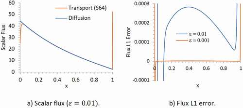
Figure 1 shows the results of the analytical solution and diffusion solution. Figure 1a plots the scalar flux for $\epsilon =0.01$ showing an excellent agreement between the two solutions in the interior region of the slab. The boundary layers develop in the transport solution on both sides of the slab due to the anisotropic BCs. Figure 1b shows that the flux L1 error (transport – diffusion) decreases with $\epsilon$. For the case of $\epsilon =0.001$, the flux L1 error is on the order of ${10}^{-6}$ in the interior region. This model problem demonstrates that the S_N analytical solution asymptotically tends to the diffusion solution in the diffusion limit, and the diffusion BCs calculated by Eqs. (66a)(66a) $\begin{array}{rl}\varphi \left(0\right)=& \frac{Q}{{\mathrm{\Sigma }}_t\left(1-c\right)}-{\mathbb{W}}^T\mathbf{R}\left[\begin{array}{cc}\mathbf{C}& \hspace{0.17em}\\ \hspace{0.17em}& \mathbf{D}\end{array}\right]\\ & {\mathbf{R}}^{-1}\left(\frac{Q}{2}\frac{1}{{\mathrm{\Sigma }}_t\left(1-c\right)}\mathbf{1}-\mathbf{R}\left[\begin{array}{c}{\mathbb{Y}}_{+}^0\\ {\mathbb{Y}}_{-}^L\end{array}\right]\right)\end{array}$(66a) and (66b(66b) $\begin{array}{rl}\varphi \left(L\right)=& \frac{Q}{{\mathrm{\Sigma }}_t\left(1-c\right)}-{\mathbb{W}}^T\mathbf{R}\left[\begin{array}{cc}\mathbf{D}& \hspace{0.17em}\\ \hspace{0.17em}& \mathbf{C}\end{array}\right]\\ & {\mathbf{R}}^{-1}\left(\frac{Q}{2}\frac{1}{{\mathrm{\Sigma }}_t\left(1-c\right)}\mathbf{1}-\mathbf{R}\left[\begin{array}{c}{\mathbb{Y}}_{+}^0\\ {\mathbb{Y}}_{-}^L\end{array}\right]\right),\end{array}$(66b) ) give a very accurate diffusion solution. However, the diffusion BCs proposed by Habetler and Matkowsky would give large differences for this case.

Fig. 1. Analytical solution vs. diffusion solution

V. CONCLUSIONS

We have presented a new proof of the asymptotic diffusion limit of the S_N transport equation by directly showing that the S_N analytical solution satisfies the diffusion equation in the asymptotic diffusion limit. The proof is made possible by showing that the smallest eigenvalue of the transport matrix tends to a constant (which is the inverse of the diffusion length), while other eigenvalues increase on the order of $O\left(1/\epsilon \right)$, and thus, their contribution to the diffusion solution in the interior of the domain can be neglected. It is natural to find the BCs for the diffusion equation when the analytical transport solution is available. It is noted that there is a deficiency in the BCs derived by Habetler and Matkowsky based on the boundary layer analysis technique. In the strict sense, they are valid only for half-space source-free transport problems in the diffusion limit (i.e., ε = 0) and would be inappropriate for inhomogeneous problems in a finite domain like slab geometry. We have demonstrated with a numerical example that the S_N analytical solution asymptotically tends to the diffusion solution.

Acknowledgments

We thank the anonymous reviewers whose comments/suggestions helped improve and clarify this manuscript.

References

- E. W. LARSEN and J. B. KELLER, “Asymptotic Solution of Neutron Transport Problems for Small Mean Free Paths,” J. Math. Phys., 15, 1, 75 (1974); https://doi.org/https://doi.org/10.1063/1.1666510.
- G. J. HABETLER and B. J. MATKOWSKY, “Uniform Asymptotic Expansion in Transport Theory with Small Mean Free Paths, and the Diffusion Approximation,” J. Math. Phys., 16, 846 (1974); https://doi.org/https://doi.org/10.1063/1.522618.
- G. C. PAPANICOLAOU, “Asymptotic Analysis of Transport Processes,” Bull. Am. Math. Soc., 81, 2, 330 (1975); https://doi.org/https://doi.org/10.1090/S0002-9904-1975-13744-X.
- E. W. LARSEN, “Diffusion Theory as an Asymptotic Limit of Transport Theory for Nearly Critical Systems with Small Mean Free Paths,” Ann. Nucl. Energy, 7, 4–5, 249 (1980); https://doi.org/https://doi.org/10.1016/0306-4549(80)90072-9.
- E. W. LARSEN, G. C. POMRANING, and V. C. BADHAM, “Asymptotic Analysis of Radiative Transfer Problems,” J. Quant. Spectrosc. Radiat. Transfer, 29, 4, 285 (1983); https://doi.org/https://doi.org/10.1016/0022-4073(83)90048-1.
- E. W. LARSEN, J. E. MOREL, and W. F. MILLER Jr., “Asymptotic Solutions of Numerical Transport Problems in Optically Thick, Diffusive Regimes,” J. Comput. Phys., 69, 2, 283 (1987); https://doi.org/https://doi.org/10.1016/0021-9991(87)90170-7.
- E. W. LARSEN and J. E. MOREL, “Asymptotic Solutions of Numerical Transport Problems in Optically Thick, Diffusive Regimes II,” J. Comput. Phys., 83, 1, 212 (1989); https://doi.org/https://doi.org/10.1016/0021-9991(89)90229-5.
- E. W. LARSEN, “The Asymptotic Diffusion Limit of Discretized Transport Problems,” Nucl. Sci. Eng., 112, 4, 336 (1992); https://doi.org/https://doi.org/10.13182/NSE92-A23982.
- M. L. ADAMS, “Discontinuous Finite Element Transport Solutions in Thick Diffusive Problems,” Nucl. Sci. Eng., 137, 3, 298 (2001); https://doi.org/https://doi.org/10.13182/NSE00-41.
- D. WANG, “The Asymptotic Diffusion Limit of Numerical Schemes for the SN Transport Equation,” Nucl. Sci. Eng., 193, 12, 1339 (2019); https://doi.org/https://doi.org/10.1080/00295639.2019.1638660.
- D. WANG and T. BYAMBAAKHUU, “A New Analytical SN Solution in Slab Geometry,” Trans. Am. Nucl. Soc., 117, 757 (2017).
- S. CHANDRASEKHAR, Radiative Transfer, Dover (1960).
- K. STAMNES and R. A. SWANSON, “A New Look at the Discrete Ordinate Method for Radiative Transfer Calculations in Anisotropically Scattering Atmospheres,” J. Atmos. Sci., 38, 387 (1981); https://doi.org/https://doi.org/10.1175/1520-0469(1981)038<0387:ANLATD>2.0.CO;2.
- K. STAMNES and P. CONKLIN, “A New Multi-Layer Discrete Ordinate Approach to Radiative Transfer in Vertically Inhomogeneous Atmospheres,” J. Quant. Spectrosc. Radiat. Transfer, 31, 3, 273 (1984); https://doi.org/https://doi.org/10.1016/0022-4073(84)90031-1.
- T. NAKAJIMA and M. TANAKA, “Matrix Formulation for the Transfer of Solar Radiation in a Plane-Parallel Scattering Atmosphere,” J. Quant. Spectrosc. Radiat. Transfer, 35, 1, 13 (1986); https://doi.org/https://doi.org/10.1016/0022-4073(86)90088-9.
- C. E. SIEWERT, “A Concise and Accurate Solution to Chandrasekhar’s Basic Problem in Radiative Transfer,” J. Quant. Spectrosc. Radiat. Transfer, 64, 2, 109 (2000); https://doi.org/https://doi.org/10.1016/S0022-4073(98)00144-7.
- J. S. WARSA, “Analytical SN Solutions in Heterogeneous Slabs Using Symbolic Algebra Computer Programs,” Ann. Nucl. Energy, 29, 7, 851 (2002); https://doi.org/https://doi.org/10.1016/S0306-4549(01)00080-9.
- B. D. GANAPOL, “The Response Matrix Discrete Ordinates Solution to the 1D Radiative Transfer Equation,” J. Quant. Spectrosc. Radiat. Transfer, 154, 72 (2015); https://doi.org/https://doi.org/10.1016/j.jqsrt.2014.11.006.
- D. S. EFREMENKO et al., “A Review of the Matrix-Exponential Formalism in Radiative Transfer,” J. Quant. Spectrosc. Radiat. Transfer, 196, 17 (2017); https://doi.org/https://doi.org/10.1016/j.jqsrt.2017.02.015.
- Multiprecision Computing Toolbox for MATLAB; https://www.advanpix.com ( current as of Oct. 11, 2020).
- Z. WU, “Extending Wang’s 1D Sn Analytic Solution to Heterogeneous Problems with No Iteration on Interfacial Fluxes,” Trans. Am. Nucl. Soc., 121 (2019); https://doi.org/https://doi.org/10.13182/T30953.
- J. ROCHELEAU and D. WANG, “A Novel Analytical Nodal Method for Solution of the SN Transport Equation,” Trans. Am. Nucl. Soc., 122, 375 (2020); https://doi.org/https://doi.org/10.13182/T122-31951.
- W. H. PRESS et al., “Sherman-Morrison Formula,” Numerical Recipes in FORTRAN: The Art of Scientific Computing, 2nd ed., Cambridge University Press (1992).
- B. DAVISON, Neutron Transport Theory, Oxford University Press, London (1957).
- I. KUSCER and I. VIDAV, “On the Spectrum of Relaxation Lengths of Neutron Distributions in a Moderator,” J. Math. Anal. Appl., 25, 80 (1969); https://doi.org/https://doi.org/10.1016/0022-247X(69)90214-5.
- K. M. CASE, “Elementary Solutions of the Transport Equation and Their Applications,” Ann. Phys., 9, 1, 1 (1960); https://doi.org/https://doi.org/10.1016/0003-4916(60)90060-9.
- K. M. CASE and P. F. ZWEIFEL, Linear Transport Theory, Addison-Wesley, Reading, Massachusetts (1967).
- D. WANG, “Diffusion Theory for Inhomogeneous Neutron Transport Problems in Slab Geometry,” Trans. Am. Nucl. Soc., 124, 196 (2021); https://doi.org/https://doi.org/10.13182/T124-34786.
- R. DAUTRAY and J.-L. LIONS, Mathematical Analysis and Numerical Methods for Science and Technology, Volume 6 Evolution Problems II, Springer-Verlag (2000).