Direct Comparison of High-Order/Low-Order Transient Methods on the 2D-LRA Benchmark Problem

Abstract

Transient simulations of nuclear systems face the computational challenge of resolving both space and time during reactivity changes. A common strategy for tackling this issue is to split the neutron flux into shape and amplitude functions. This split can be solved with high-order/low-order methods. In this paper, a direct comparison of commonly used approximations (e.g., adiabatic, omega, alpha eigenvalue, frequency transform, quasi-static) is performed on the two-dimensional Laboratorium für Reaktorregelung und Anlagensicherung (2D-LRA) benchmark problem using a diffusion solver as the high-order solver and point kinetics as the low-order solver. Additionally, a novel hybrid omega/alpha-eigenvalue solver that incorporates frequencies to model delayed neutrons is introduced. The goal of the comparison is to quantify the performance of each method on a common problem to help inform promising pathways for costly high-fidelity solvers. Overall, we show that exponential frequency approximations are an effective strategy for increasing the accuracy of transient simulations with no added cost. Root-mean-square error of the power distribution at the peak of the transient was consistently decreased by 20% by including frequencies. In particular, the hybrid omega/alpha-eigenvalue method shows improvement over existing eigenvalue solvers as a high-order method. However, in our implementation, the cost of solving for the alpha eigenmode is too costly to recommend over the omega method. While time-differencing schemes are more accurate, we believe the eigenvalue methods are more adaptable to further applications in Monte Carlo transients. Furthermore, they required fewer outer time steps, significantly reducing the computational cost.

Keywords:

• High-order/low-order methods
• transients
• alpha eigenvalue
• frequency transform
• improved quasi-static method

I. INTRODUCTION

Modern numerical methods have resulted in a large variety of accurate and efficient solvers for neutron transport steady-state calculations, each with their own approximations catered toward specific applications. Similarly, there exist many methods for computing time-dependent problems, as the nature of the transient impacts the accuracy of each approximation. In time-dependent problems, the biggest challenge is developing a good approximation to time derivative terms.

While Monte Carlo is an attractive method for high-fidelity calculations, it still encounters a prohibitive computational barrier for modeling transients due to the introduction of delayed neutron precursors. While the concept of taking steady-state Monte Carlo to transient is very straightforward, the implementation is so expensive that current time-dependent Monte Carlo methods are limited to transients of under 1 s (Refs. 1, 2, and 3). To resolve transients of more than 1 s with Monte Carlo, it is feasible to employ a high-order/low-order (HOLO) method. This category of solver pairs a high-fidelity solver with a more rudimentary one to accelerate the solution. Sometimes, HOLO methods are used at steady state to resolve fine mesh problems in a multigrid scheme.^4–7 In time-dependent problems, the high-order method is used periodically to resolve the details of the flux, including shape, while the low-order method advances the problem in time by approximating the flux shape and focusing instead on the amplitude. Despite the many varieties of HOLO transient methods available, there are not any comprehensive, direct comparisons between them. In this paper, several HOLO transient methods will be compared against each other on a common reactor benchmark.

Historically, alpha-eigenvalue methods have dominated transient methods as a way to model the time absorption of neutrons. However, most formulations of the alpha eigenvalue are not ideal for modeling delayed neutrons, which are essential to reactor-relevant transients. In this paper, a novel approach that uses frequencies to model delayed neutron precursors within the alpha-eigenvalue method is being proposed to bring an increased level of accuracy to alpha-eigenvalue methods for reactor transients.

The methods in this comparative study include several eigenvalue methods: a fixed shape method for illustration only; the adiabatic method, which is commonly used; the omega method, which is an improvement on the adiabatic method; and the alpha-eigenvalue method. The alpha-eigenvalue method is presented in different modes, including our novel hybrid mode where the omega and alpha-eigenvalue methods are combined to improve precursor resolution. We also compare several time-differencing methods: the frequency transform method (FTM), a coarse time integration, and the improved quasi-static (IQS) method. The goal is to directly compare the accuracy of these methods on a common problem and establish a clear flowchart of how these methods are related to each other. As such, the solvers chosen can be simple. The high-order solver selected is two-dimensional (2D) diffusion, and the low-order solver is point kinetics. The conclusions of this paper will aim to inform modern research applications, for example, by being extended to high-fidelity methods such as Monte Carlo using coarse mesh finite difference as the low-order method.^8,9

II. METHODS

II.A. Reference Solution

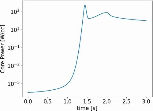
The comparison problem is the 2D Laboratorium für Reaktorregelung und Anlagensicherung LRA (2D-LRA) transient benchmark of a boiling water reactor (BWR) quarter-core in which a control rod is withdrawn.¹⁰ The geometry is a BWR quarter-core with assemblies that are 15 × 15 cm. The control rod is withdrawn in the region noted R in Fig. 1. As the control rod is removed, there is thermal feedback in the system that causes the power spike to stabilize, as illustrated in Fig. 2. See the full description of this numerical benchmark in Appendix A, along with an important note about values that differ from the original benchmark specification.

Fig. 1. 2D-LRA geometry.¹¹

Fig. 2. Example power evolution during the 2D-LRA transient on a 1 cm mesh.

II.A.1. Steady-State Solution

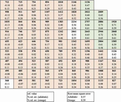
The steady-state problem must be solved to obtain initial values. Our steady-state two-group diffusion calculation was found to be spatially converged with a uniform 1 cm mesh. Our results are compared to computational results in the literature.¹² Our steady-state eigenvalue was within 4 pcm of the reference, and the maximum error in normalized assembly-averaged power was below 1% relative error as shown in Fig. 3. These results demonstrate that our code accurately depicts the geometry and steady-state solution of the benchmark.

Fig. 3. Assembly power densities normalized to 1 W/cm³ at steady state, error with respect to results by Smith.¹²

II.A.2. Transient Solution

The two-group time-dependent diffusion equations, coupled with the precursor balance equations, are discretized in space and time and solved using the previously listed HOLO methods. There is little information in the literature about transient benchmark results for fine spatial mesh solutions of the 2D-LRA benchmark. Most transient reference solutions utilize coarse mesh nodal methods, mostly on 15 cm meshes. While nodal methods can finely resolve flux, the feedback effects and cell details are assembly-averaged throughout the transient, which does not make a sufficiently detailed reference solution compared to finite difference. Therefore, our reference for the transient problem is a highly refined run of our own fully implicit solver.¹³

Our code uses an implicit time scheme with first-order temporal differencing. Since the transient cross sections are prescribed, it is possible to update the cross sections before solving for ${\mathrm{\Psi }}^{n+1}$. However, since the cross-section change induced by Doppler feedback relies on the new temperature (see Appendix A), and therefore the new fission reaction rate, there is a lag. It is minor enough to avoid needing a leapfrog method given small time steps (0.01 s or smaller).

Some problems are conducive to using higher-order differencing methods such as backward differencing of the second order (BD2, otherwise known as Crank-Nicolson). However, proof of higher-order convergence is limited to cases with constant matrix properties. In a transient problem, where the matrix changes at every time step, higher-order convergence is rarely observed; thus, a backward differencing of the first order (BD1) approach will be used:

(1) $\frac{df}{dt}=\frac{1}{\mathrm{\Delta }t}\left(f^{n+1}-f^n\right)+O\left(\mathrm{\Delta }t\right).$(1)

The diffusion equation, in mesh-centered finite difference with cell-averaged properties, discretized in time in an implicit scheme is

(2) $\begin{array}{rl}& \frac{1}{v_g}\frac{{\mathrm{\Psi }}_g^{n+1}-{\mathrm{\Psi }}_g^n}{\mathrm{\Delta }t}=\mathrm{\nabla }\cdot D_g^{n+1}\mathrm{\nabla }{\mathrm{\Psi }}_g^{n+1}-\left[{\mathrm{\Sigma }}_{rg}^{n+1}\right]{\mathrm{\Psi }}_g^{n+1}\\ & \hspace{0.17em}\hspace{0.17em}\hspace{0.17em}\hspace{0.17em}\hspace{0.17em}\hspace{0.17em}\hspace{0.17em}\hspace{0.17em}\hspace{0.17em}\hspace{0.17em}\hspace{0.17em}\hspace{0.17em}\hspace{0.17em}\hspace{0.17em}+\sum _{g^{\prime }\ne g}{\mathrm{\Sigma }}_{s{g}^{\prime }\to g}^{n+1}{\mathrm{\Psi }}_{g^{\prime }}^{n+1}+\left(1-{\beta }_{tot}\right)\frac{{\chi }_g^P}{k_{crit}}\hspace{0.17em}\hspace{0.17em}\hspace{0.17em}\hspace{0.17em}\hspace{0.17em}\hspace{0.17em}\hspace{0.17em}\hspace{0.17em}\hspace{0.17em}\sum _{g^{\prime }}{\nu }_{g^{\prime }}{\mathrm{\Sigma }}_{f{g}^{\prime }}^{n+1}{\mathrm{\Psi }}_{g^{\prime }}^{n+1}\hspace{0.17em}\hspace{0.17em}\hspace{0.17em}\hspace{0.17em}\hspace{0.17em}\\ & \hspace{0.17em}\hspace{0.17em}\hspace{0.17em}+\sum _i{\chi }_g^D{\lambda }_i{C}_i^{n+1},& (2)\end{array}$(2)

with

(3) $\begin{array}{c}\frac{d{C}_i\left(t\right)}{dt}=-{\lambda }_i{C}_i\left(t\right)+\frac{{\beta }_i}{k_{crit}}\sum _{g^{\prime }}{\nu }_{g{ }^{\mathrm{\prime }}}{\mathrm{\Sigma }}_{fg{ }^{\mathrm{\prime }}}\left(t\right){\mathrm{\Psi }}_{g^{\prime }}\left(t\right).\end{array}$(3)

The constant k_crit represents the value of k_eff in the initial state of the reactor. Since reactor models are not necessarily exactly critical, the transient equations must scale by k_crit to guarantee that a steady-state solution can be maintained if no perturbations are made.

By assuming that the flux shape changes linearly over the time step, the precursor equation has an analytic solution that removes much of the error associated with the time discretization of the precursor concentrations. This derivation is detailed in Appendix B for the FTM. To apply those equations to the implicit method, set $\omega =0$ to obtain Eq. (4$\begin{array}{rl}& C_i^{n+1}=C_i^n{e}^{-{\lambda }_i\mathrm{\Delta }t}+\frac{{\beta }_i}{k_{crit}{\lambda }_i}\sum _{g^{\prime }}{\nu }_{g^{\prime }}{\mathrm{\Sigma }}_{f{g}^{\prime }}\\ & \left[{\mathrm{\Psi }}_{g^{\prime }}^n\left(-e^{-{\lambda }_i\mathrm{\Delta }t}+\frac{1-e^{-{\lambda }_i\mathrm{\Delta }t}}{{\lambda }_i\mathrm{\Delta }t}\right)\right.\\ & \left.+{\mathrm{\Psi }}_{g^{\prime }}^{n+1}\left(1-\frac{1-e^{-{\lambda }_i\mathrm{\Delta }t}}{{\lambda }_i\mathrm{\Delta }t}\right)\right].(4)\end{array}$), which matches Bandini’s equation (5.7) (Ref. 14):

$\begin{array}{rl}& C_i^{n+1}=C_i^n{e}^{-{\lambda }_i\mathrm{\Delta }t}+\frac{{\beta }_i}{k_{crit}{\lambda }_i}\sum _{g^{\prime }}{\nu }_{g^{\prime }}{\mathrm{\Sigma }}_{f{g}^{\prime }}\\ & \left[{\mathrm{\Psi }}_{g^{\prime }}^n\left(-e^{-{\lambda }_i\mathrm{\Delta }t}+\frac{1-e^{-{\lambda }_i\mathrm{\Delta }t}}{{\lambda }_i\mathrm{\Delta }t}\right)\right.\\ & \left.+{\mathrm{\Psi }}_{g^{\prime }}^{n+1}\left(1-\frac{1-e^{-{\lambda }_i\mathrm{\Delta }t}}{{\lambda }_i\mathrm{\Delta }t}\right)\right].(4)\end{array}$

Substituting into the diffusion Eqs. (2)(2) $\begin{array}{rl}& \frac{1}{v_g}\frac{{\mathrm{\Psi }}_g^{n+1}-{\mathrm{\Psi }}_g^n}{\mathrm{\Delta }t}=\mathrm{\nabla }\cdot D_g^{n+1}\mathrm{\nabla }{\mathrm{\Psi }}_g^{n+1}-\left[{\mathrm{\Sigma }}_{rg}^{n+1}\right]{\mathrm{\Psi }}_g^{n+1}\\ & \hspace{0.17em}\hspace{0.17em}\hspace{0.17em}\hspace{0.17em}\hspace{0.17em}\hspace{0.17em}\hspace{0.17em}\hspace{0.17em}\hspace{0.17em}\hspace{0.17em}\hspace{0.17em}\hspace{0.17em}\hspace{0.17em}\hspace{0.17em}+\sum _{g^{\prime }\ne g}{\mathrm{\Sigma }}_{s{g}^{\prime }\to g}^{n+1}{\mathrm{\Psi }}_{g^{\prime }}^{n+1}+\left(1-{\beta }_{tot}\right)\frac{{\chi }_g^P}{k_{crit}}\hspace{0.17em}\hspace{0.17em}\hspace{0.17em}\hspace{0.17em}\hspace{0.17em}\hspace{0.17em}\hspace{0.17em}\hspace{0.17em}\hspace{0.17em}\sum _{g^{\prime }}{\nu }_{g^{\prime }}{\mathrm{\Sigma }}_{f{g}^{\prime }}^{n+1}{\mathrm{\Psi }}_{g^{\prime }}^{n+1}\hspace{0.17em}\hspace{0.17em}\hspace{0.17em}\hspace{0.17em}\hspace{0.17em}\\ & \hspace{0.17em}\hspace{0.17em}\hspace{0.17em}+\sum _i{\chi }_g^D{\lambda }_i{C}_i^{n+1},& (2)\end{array}$(2) and (3(3) $\begin{array}{c}\frac{d{C}_i\left(t\right)}{dt}=-{\lambda }_i{C}_i\left(t\right)+\frac{{\beta }_i}{k_{crit}}\sum _{g^{\prime }}{\nu }_{g{ }^{\mathrm{\prime }}}{\mathrm{\Sigma }}_{fg{ }^{\mathrm{\prime }}}\left(t\right){\mathrm{\Psi }}_{g^{\prime }}\left(t\right).\end{array}$(3) ) and assuming two energy groups, the group 1 equation is

(5) $\begin{array}{rl}& -\mathrm{\nabla }\cdot D_1\mathrm{\nabla }{\mathrm{\Psi }}_1^{n+1}+[{\mathrm{\Sigma }}_{r1}+\frac{1}{v_1\mathrm{\Delta }t}]{\mathrm{\Psi }}_1^{n+1}\\ & -\left[\frac{\left(1-{\beta }_{tot}\right)}{k_{crit}}+\sum _i{\lambda }_i\frac{{\beta }_i}{k_{crit}{\lambda }_i}\left(1-\frac{1-e^{-{\lambda }_i\mathrm{\Delta }t}}{{\lambda }_i\mathrm{\Delta }t}\right)\right]\\ & \left[{\nu }_1{\mathrm{\Sigma }}_{f1}{\mathrm{\Psi }}_1^{n+1}+{\nu }_2{\mathrm{\Sigma }}_{f2}{\mathrm{\Psi }}_2^{n+1}\right]\\ & =\sum _i{\lambda }_i\frac{{\beta }_i}{k_{crit}{\lambda }_i}\left(-e^{-{\lambda }_i\mathrm{\Delta }t}+\frac{1-e^{-{\lambda }_i\mathrm{\Delta }t}}{{\lambda }_i\mathrm{\Delta }t}\right)\\ & \left[{\nu }_1{\mathrm{\Sigma }}_{f1}{\mathrm{\Psi }}_1^n+{\nu }_2{\mathrm{\Sigma }}_{f2}{\mathrm{\Psi }}_2^n\right]+\sum _i{\lambda }_i{C}_i^n{e}^{-{\lambda }_i\mathrm{\Delta }t}+\frac{{\mathrm{\Psi }}_1^n}{v_1\mathrm{\Delta }t},\end{array}$(5)

and the group 2 equation is

(6) $\begin{array}{c}-\mathrm{\nabla }\cdot D_2\mathrm{\nabla }{\mathrm{\Psi }}_2^{n+1}+\left[{\mathrm{\Sigma }}_{a2}+\frac{1}{v_2\mathrm{\Delta }t}\right]{\mathrm{\Psi }}_2^{n+1}-{\mathrm{\Sigma }}_{s1\to 2}{\mathrm{\Psi }}_1^{n+1}=\frac{{\mathrm{\Psi }}_2^n}{v_2\mathrm{\Delta }t},\end{array}$(6)

which can be rewritten as

(7) $\begin{array}{c}\left\{\begin{array}{c}-\mathrm{\nabla }\cdot D_1^{n+1}\mathrm{\nabla }{\mathrm{\Psi }}_1^{n+1}+\widehat{{\mathrm{\Sigma }}_{r1}^{n+1}}{\mathrm{\Psi }}_1^{n+1}-\sum _{g^{\prime }}\widehat{{\mathrm{\Sigma }}_{f{g}^{\prime }}^{n+1}}{\mathrm{\Psi }}_{g^{\prime }}^{n+1}=S_1\\ -\mathrm{\nabla }\cdot D_2^{n+1}\mathrm{\nabla }{\mathrm{\Psi }}_2^{n+1}+\widehat{{\mathrm{\Sigma }}_{r2}^{n+1}}{\mathrm{\Psi }}_2^{n+1}-{\mathrm{\Sigma }}_{s1\to 2}^{n+1}{\mathrm{\Psi }}_1^{n+1}=S_2\end{array}\right.,\end{array}$(7)

where the modified cross sections account for the additional terms including the time discretization terms and the analytic precursor terms. This form resembles steady-state equations, allowing us to solve each step in the transient problem similarly to a flux matrix inversion in fission source iteration. We use a Gauss-Seidel iteration scheme to do so with very tight convergence criterion of 10⁻¹⁰.

The transient problem on a 1 cm mesh was evaluated for temporal convergence using time steps of 10⁻⁵, 10⁻⁴, and 10⁻³ s. The sensitivities of the results to the time step size are presented in Table I. The finest run is used as the reference in this paper. These results support a linear convergence rate.

TABLE I Sensitivity of the Transient Results on Time Step Size: Comparison with a Fine-Time Solution

	10^−5 s Solution	10^−4 s (Percent Relative Difference)	10^−3 s (Percent Relative Difference)
Time to first peak (s)	1.44545	0.04	0.45
Power at first peak (W/cm^3)	5448.7	0.03	0.43
Power at second peak (W/cm^3)	792.80	0.05	0.16
Power at t = 3 s (W/cm^3)	98.06	0.02	0.12

The times and power values reported in Table I are the global comparison metrics that will be used throughout this paper to compare numerical methods against each other. A spatial comparison will also be performed on the normalized assembly-averaged power at the power peak and the assembly-averaged temperatures at 3 s.

II.B. Description of Point Kinetics as the Low-Order Method

In HOLO schemes, the high-order method is carried out over long outer time steps and the low-order method over short inner time steps (marked in blue and green in Fig. 4, respectively).

Fig. 4. Time stepping scheme for transient HOLO methods.

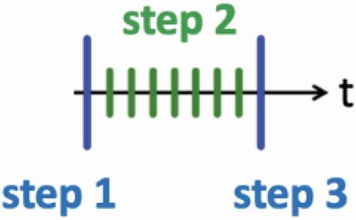
It is assumed that the flux shape is slowly changing, so it can be updated at the infrequent outer steps, while the amplitude is quickly changing, so it is updated often on the inner steps. Decomposing flux into shape and amplitude components,

(8) $\begin{array}{c}\mathrm{\Psi }\left(r,E,t\right)=\psi \left(r,E,t\right)\varphi \left(t\right),\end{array}$(8)

where

$\mathrm{\Psi }$	=	= full flux
$\psi$	=	= shape function
$\varphi$	=	= amplitude function.

The point kinetics equations (PKEs) assume that the amplitude is only a time-dependent scalar $\varphi \left(t\right)$, resulting in no spatial resolution on the amplitude. However, the shape function, which can be updated at every outer time step, can be used to calculate PKE parameters. In this paper, two outer time steps are solved, and the resulting shape functions are interpolated for increased accuracy and some spatial resolution on the inner time steps. In terms of Fig. 4, the procedure is the following:

1. Step 1: initial shape calculation

2. Step 2: amplitude calculation, assuming constant shape

3. Step 3: next-step shape calculation

4. Repeat Step 2: amplitude calculation, using interpolated shape.

In fact, this interpolation could be repeated in a loop until a converged result is achieved, but this is not implemented in order to compare methods fairly with a constant number of outer step iterations.

There are many ways to compute PKE parameters. In this work, they are derived from the two-group diffusion equations. The flux shape $\psi$ is from the most recent shape calculation or interpolated between outer steps while the amplitude $\varphi$ is from the previous inner time step. Additionally, an adjoint flux weighting $\psi \ast$ is used. In the eigenvalue methods below, the adjoint is updated every time the flux shape is updated, so the adjoint used is the adjoint of the new shape, as done by Wu et al.¹⁵ This differs from some implementations where only the beginning-of-life adjoint is used, which is a more arbitrary weighting factor.^16,17 However, in the time-differencing methods, the beginning-of-life adjoint weighting is used to avoid including an eigenvalue solver in addition to a time-differencing solver. Thus, the reactivity insertion at each inner step is computed as

(9) $\rho (t)=\frac{\begin{array}{c}\int dr{\psi }_1^{\ast }(r,t)\left\{-{\mathrm{\Sigma }}_{r1}(r,t){\psi }_1(r,t)\varphi (t)+{\sum }_{g^{\prime }=1}^2\hspace{0.17em}\right.\\ \left.\hspace{0.17em}{\nu }_{g^{\prime }}{\mathrm{\Sigma }}_{f{g}^{\prime }}(r,t){\psi }_{g^{\prime }}(r,t)\varphi (t)/k_{crit}\right\}\\ +\int dr{\mathrm{\Psi }}_2^{\ast }(r,t)\left\{-{\mathrm{\Sigma }}_{\alpha 2}(r,t){\psi }_2(r,t)\varphi (t)\right.\\ \left.+{\mathrm{\Sigma }}_{s1\to 2}(r,t){\psi }_2(r,t)\varphi (t)\right\}\end{array}}{\int dr{\psi }_1^{\ast }(r,t){\sum }_{g^{\prime }=1}^2{\nu }_{g^{\prime }}{\mathrm{\Sigma }}_{f{g}^{\prime }}(r,t){\psi }_{g^{\prime }}(r,t)/k_{crit}},\hspace{0.17em}$(9)

and the prompt neutron lifetime is computed as

(10) $\Lambda \left(t\right)={\displaystyle \int d}r\frac{1}{v_1}{\psi }_1\left(r,t\right){\psi }_1^{*}\left(r,t\right)+\frac{1}{v_2}{\psi }_2\left(r,t\right){\psi }_2^{*}\left(r,t\right){\displaystyle \int d}r{\psi }_1^{*}\left(r,t\right)\sum g\prime =12{\nu }_{g^{\prime }}{\Sigma }_{f{g}^{\prime }}\left(r,t\right){\psi }_{g^{\prime }}\left(r,t\right)/k_{crit}.$(10)

These terms are then inserted into the PKEs:

(11) $\begin{array}{c}\frac{d}{dt}\varphi \left(t\right)=\frac{\rho \left(t\right)-{\sum }_i{\beta }_i}{\mathrm{\Lambda }\left(t\right)}\varphi \left(t\right)+\sum _i{\lambda }_i{C}_i\left(t\right)+S\left(t\right)\end{array}$(11)

and

(12) $\begin{array}{c}\frac{d}{dt}{C}_i\left(t\right)=\frac{{\beta }_{\mathrm{i}}}{\mathrm{\Lambda }\left(t\right)}\varphi \left(t\right)-{\lambda }_i{C}_i\left(t\right).\end{array}$(12)

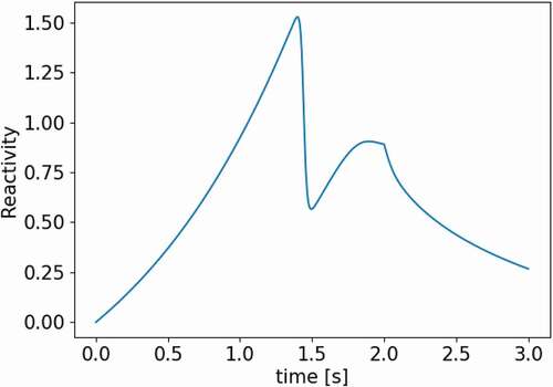
Defined in this way, the PKEs are then solved using a high-order Pade approximation exponential matrix function in the scipy.linalg library in Python.¹⁸ Figure 5 illustrates the reactivity change during the 2D-LRA transient.

Fig. 5. Example reactivity evolution during the 2D-LRA transient on a 1 cm mesh.

With two-group 2D diffusion as the high-order method and PKEs as the low-order method, we now present the list of HOLO methods used in this comparison study. Two broad categories are distinguished: eigenvalue methods and time-differencing methods. All methods are carried out on a variation of the time stepping scheme of Fig. 4. This summary of methods focuses on their differences, mostly revolving around approximations to time derivatives in the high-order method.

II.C. Eigenvalue Methods

The following methods employ some form of eigenvalue solver to calculate the flux shape updates. The PKEs are the main driver of the transient, occurring at every inner time step to update the power, calculate all feedback parameters, and compute a spatial distribution of precursor concentrations using the interpolation of the flux shape between outer time steps.

II.C.1. Fixed Shape Method

The fixed shape method is a very rudimentary method whereby the beginning-of-life flux shape is used throughout the PKE transient calculation without any updates. This method illustrates the importance of periodic shape function updates. The sole shape calculation is governed by the following k-eigenvalue equation, solved by power iteration, with all time-dependent terms at time step 0, hence the superscript. The time derivatives are absent because the equation is at steady-state

$\begin{array}{rl}& -\mathrm{\nabla }\cdot D_g^0\mathrm{\nabla }{\psi }_g^0+\left[{\mathrm{\Sigma }}_{rg}^0\right]{\psi }_g^0-\sum _{g^{\prime }\ne g}{\mathrm{\Sigma }}_{s{g}^{\prime }\to g}^0{\psi }_{g^{\prime }}^0\\ & =\frac{\mathbf{1}}{\mathit{k}}\left[\frac{\left(1-{\beta }_{tot}\right)}{k_{crit}}{\chi }_g^P+\sum _i\frac{{\chi }_g^D}{k_{crit}}\frac{{\beta }_i{\lambda }_i}{{\lambda }_i}\right]\\ & \sum _{g^{\prime }}{\nu }_{g^{\prime }}{\mathrm{\Sigma }}_{f{g}^{\prime }}^0{\psi }_{g^{\prime }}^0(13)\end{array}$

$\begin{array}{rl}& \Rightarrow -\mathrm{\nabla }\cdot D_g^0\mathrm{\nabla }{\psi }_g^0+\left[{\mathrm{\Sigma }}_{rg}^0\right]{\psi }_g^0-\sum _{g^{\prime }\ne g}{\mathrm{\Sigma }}_{s{g}^{\prime }\to g}^0{\psi }_{g^{\prime }}^0\\ & =\frac{{\chi }_g^{eq}}{\mathit{k}}\sum _{g^{\prime }}{\nu }_{g^{\prime }}{\mathrm{\Sigma }}_{f{g}^{\prime }}^0{\psi }_{g^{\prime }}^0.(14)\end{array}$

II.C.2. Adiabatic Method

In the adiabatic method, the transient is assumed to be slow enough to be approximated by instantaneous eigenstates.¹⁴ As such, the time derivatives for flux and precursor concentrations are zeroed out, much like the fixed shape method. In fact, the only difference between the fixed shape method and the adiabatic method is how often Eq. (14)$\begin{array}{rl}& -\mathrm{\nabla }\cdot D_g^0\mathrm{\nabla }{\psi }_g^0+\left[{\mathrm{\Sigma }}_{rg}^0\right]{\psi }_g^0-\sum _{g^{\prime }\ne g}{\mathrm{\Sigma }}_{s{g}^{\prime }\to g}^0{\psi }_{g^{\prime }}^0\\ & =\frac{\mathbf{1}}{\mathit{k}}\left[\frac{\left(1-{\beta }_{tot}\right)}{k_{crit}}{\chi }_g^P+\sum _i\frac{{\chi }_g^D}{k_{crit}}\frac{{\beta }_i{\lambda }_i}{{\lambda }_i}\right]\\ & \sum _{g^{\prime }}{\nu }_{g^{\prime }}{\mathrm{\Sigma }}_{f{g}^{\prime }}^0{\psi }_{g^{\prime }}^0(13)\end{array}$ is solved. In the adiabatic method, Eq. (14)$\begin{array}{rl}& -\mathrm{\nabla }\cdot D_g^0\mathrm{\nabla }{\psi }_g^0+\left[{\mathrm{\Sigma }}_{rg}^0\right]{\psi }_g^0-\sum _{g^{\prime }\ne g}{\mathrm{\Sigma }}_{s{g}^{\prime }\to g}^0{\psi }_{g^{\prime }}^0\\ & =\frac{\mathbf{1}}{\mathit{k}}\left[\frac{\left(1-{\beta }_{tot}\right)}{k_{crit}}{\chi }_g^P+\sum _i\frac{{\chi }_g^D}{k_{crit}}\frac{{\beta }_i{\lambda }_i}{{\lambda }_i}\right]\\ & \sum _{g^{\prime }}{\nu }_{g^{\prime }}{\mathrm{\Sigma }}_{f{g}^{\prime }}^0{\psi }_{g^{\prime }}^0(13)\end{array}$ changes slightly to reflect values at outer time step n + 1:

(15) $\begin{array}{rl}& -\mathrm{\nabla }\cdot D_g^{n+1}\mathrm{\nabla }{\psi }_g^{n+1}+\left[{\mathrm{\Sigma }}_{rg}^{n+1}\right]{\psi }_g^{n+1}-\sum _{g^{\prime }\ne g}{\mathrm{\Sigma }}_{s{g}^{\prime }\to g}^{n+1}{\psi }_{g^{\prime }}^{n+1}\\ & =\frac{\mathbf{1}}{\mathit{k}}\sum _{g^{\prime }}{\nu }_{g^{\prime }}{\mathrm{\Sigma }}_{f{g}^{\prime }}^{n+1}{\psi }_{g^{\prime }}^{n+1}.\end{array}$(15)

In between these shape updates, the PKEs advance the transient using interpolated shape information.

II.C.3. Omega Method

In the omega method, the shape calculation includes some time dependence. The amplitude function is approximated as an exponential:

(16) $\Psi \left(r,E,t\right)=\psi \left(r,E,t\right)e^{{\omega }^P\left(r,E,t\right)t}.$(16)

The frequency ${\omega }^P$ is computed as needed by the PKE when returning to the diffusion solver

(18) $e^{{\omega }^P\cdot \mathrm{\Delta }t}{\varphi }_{t_{n-1}}={\varphi }_{t_n}(17)\Rightarrow {\omega }^P=\frac{1}{\mathrm{\Delta }t}log\left(\frac{{\varphi }_{t_n}}{{\varphi }_{t_{n-1}}}\right).$(18)

As such, the frequencies are considered instantaneous, and therefore, their time dependence can be neglected (not because they are constant but because they are instantaneous). With this in mind, we differentiate Eq. (16)(16) $\Psi \left(r,E,t\right)=\psi \left(r,E,t\right)e^{{\omega }^P\left(r,E,t\right)t}.$(16) with respect to time:

(19) $\frac{\partial \Psi }{\partial t}=\frac{\partial \psi }{\partial t}{e}^{{\omega }^{P}t}+\psi \cdot {\omega }^P{e}^{{\omega }^{P}t}.$(19)

If the frequencies are properly chosen, the shape function is slowly varying relative to the amplitude function. In fact, since the frequencies are computed using the last inner time step before the shape calculation, they are considered quite accurate. Therefore, we approximate the derivative of the shape to be zero.^14,19 This leads to

(20) $\frac{\partial \Psi }{\partial t}=\psi \cdot {\omega }^P{e}^{{\omega }^{P}t}\Rightarrow \frac{1}{v}\frac{\partial \Psi }{\partial t}=\frac{1}{v}{\omega }^P\cdot \Psi .$(20)

Likewise, the precursor concentrations can be frequency transformed to yield

(21) $\frac{\partial C}{\partial t}={\omega }^D\cdot C,$(21)

where

(23) $e^{{\omega }^D\cdot \mathrm{\Delta }t}{C}_{t_{n-1}}=C_{t_n}(22)\Rightarrow {\omega }^D=\frac{1}{\mathrm{\Delta }t}log\left(\frac{C_{t_n}}{C_{t_{n-1}}}\right).$(23)

So, ${\omega }^{P,g}$ is the prompt neutron frequency for each energy group g, and ${\omega }^{D,i}$ is the delayed neutron frequency for each precursor group i. Both have units of inverse time and can be phase-space dependent, limited only by the precision of the low-order method. In this work, only a single prompt frequency is employed for both energy groups because we are using single-group PKEs. The prompt frequencies are not spatially distributed, which has been shown to have little impact on the accuracy of frequency-transformed problems.⁹ There is, however, much be gained from spatially distributed delayed frequencies. Therefore, the interpolated shape between outer time steps is used along with the amplitude change calculated by the PKEs to numerically integrate the precursor distribution at each inner time step. This step allows us to estimate the precursor distribution at every moment of the transient and provide spatially distributed delayed precursors to the k-eigenvalue solver at the shape updates:

(24) $-\nabla \cdot D_g{ }^{n+1}\nabla {\psi }_g{ }^{n+1}+\Sigma rgn+1+\frac{{\omega }^P(t)}{v_g}{\psi }_g{ }^{n+1}-\sum g^{\prime }\ne g\Sigma s{g}^{\prime }\to gn+1{\psi }_{g^{\prime }}{ }^{n+1}=\frac{1}{k}(1-{\beta }_{tot})k_{crit}{\chi }_g{ }^P+\sum i\frac{{\chi }_g{ }^P}{k_{crit}}{\beta }_i{\lambda }_i({\lambda }_i+{\omega }^{Di}(r,t)){\displaystyle \sum _{g^{\prime }}{\nu }_{g^{\prime }}}\Sigma f{g}^{\prime }n+1{\psi }_{g^{\prime }}{ }^{n+1}.$(24)

This form of the equation shows how the prompt frequency can be added to the removal cross section, akin to a time absorption factor as seen in alpha-eigenvalue literature. If all the frequencies are exact, the resulting value of k should be 1. We use the computed value of k and its difference from 1 to quantify the accuracy of the omega-mode implementation. As will be seen in the results, the k-balance of the omega method strays only a few pcm from 1 during the LRA transient with our selected time steps. If the frequencies are all set to 0, the method collapses to the adiabatic method.

II.C.4. Alpha-Eigenvalue Method

The alpha-eigenvalue method is of a slightly different nature than the adiabatic and omega methods but retains similarities. The alpha-eigenvalue method approximates the amplitude function as an exponential so that Eq. (16)(16) $\Psi \left(r,E,t\right)=\psi \left(r,E,t\right)e^{{\omega }^P\left(r,E,t\right)t}.$(16) becomes

(25) $\Psi \left(r,E,t\right)=\psi \left(r,E,t\right)e^{\alpha \left(t\right)\cdot t},$(25)

where $\alpha$ is very similar to ${\omega }^P$, having units of inverse time and acting as a time absorption term. Instead of calculating $\alpha$ from the PKE and passing it to the shape update, $\alpha$ is calculated during the shape update. A classic alpha-eigenvalue method is described in this work, as well as several modifications that can potentially increase accuracy in reactor-relevant transients.

II.C.4.a. Classic Alpha-Eigenvalue Method

Note that the formulation of the classic alpha-eigenvalue method neglects the role of delayed neutrons, therefore requiring prompt-only values of ${\nu }^P,{\chi }^P$ in the fission term.²⁰ This classic alpha-eigenvalue method is implemented in this work with ${\nu }^P=\nu \left(1-\beta \right)$:

$\begin{array}{rl}& -\mathrm{\nabla }\cdot D_g^{n+1}\mathrm{\nabla }{\psi }_g^{n+1}+\left[{\mathrm{\Sigma }}_{rg}^{n+1}+\frac{\mathit{\alpha }\left(\mathit{t}\right)}{v_g}\right]{\psi }_g^{n+1}\\ & -\sum _{g^{\prime }\ne g}{\mathrm{\Sigma }}_{s{g}^{\prime }\to g}^{n+1}{\psi }_{g^{\prime }}^{n+1}=\frac{{\chi }_g^P}{\mathit{k}}\sum _{g^{\prime }}{\nu }_{g^{\prime }}^P{\mathrm{\Sigma }}_{f{g}^{\prime }}^{n+1}{\psi }_{g^{\prime }}^{n+1}.(26)\end{array}$

The critical search method,²¹ as implemented by Ortega, can be used for the classic alpha-eigenvalue solver. This method has been shown to be unstable for very subcritical problems but works well otherwise. Using successive guesses for $\alpha$, values for k are found. The [$\alpha$,k] pairs are used to extrapolate to the true value of $\alpha$ such that k = 1. This method can be costly due to repeated k-eigenvalue calculations (especially when the problem is close to critical) and the need to have a very tightly converged k-eigenvalue. This k-eigenvalue can be used as a balance term to determine the accuracy of the $\alpha$ values like in the omega method.

II.C.4.b. Modified Alpha-Eigenvalue Method

In the presence of delayed neutrons, a modification must be made to the classic alpha-eigenvalue formulation. Here, we include $\alpha$ as a precursor frequency and solve for $\alpha$ using the same algorithm as above. Remember that k is forced to be 1 as described in the critical search method. A derivation of Eq. (27)(28) $-\nabla \cdot D_g{ }^{n+1}\nabla {\psi }_g{ }^{n+1}+\Sigma rgn+1+\frac{\alpha (t)}{v_g}{\psi }_g{ }^{n+1}-\sum g^{\prime }\ne g\Sigma s{g}^{\prime }\to gn+1{\psi }_{g^{\prime }}{ }^{n+1}=\frac{1}{k}(1-{\beta }_{tot})k_{crit}{\chi }_g{ }^P+\sum i\frac{{\chi }_g{ }^D}{k_{crit}}{\beta }_i{\lambda }_i({\lambda }_i+{\omega }^{Di}(r,t){\displaystyle \sum _{g^{\prime }}{\nu }_{g^{\prime }}}\Sigma f{g}^{\prime }n+1{\psi }_{g^{\prime }}{ }^{n+1}.$(28) has been published by Josey and Brown²²:

$-\nabla \cdot D_g{ }^{n+1}\nabla {\psi }_g{ }^{n+1}+\Sigma rgn+1+\frac{\alpha (t)}{v_g}{\psi }_g{ }^{n+1}-\sum g^{\prime }\ne g\Sigma s{g}^{\prime }\to gn+1{\psi }_{g^{\prime }}{ }^{n+1}=\frac{1}{k}(1-{\beta }_{tot})k_{crit}{\chi }_g{ }^P+\sum i\frac{{\chi }_g{ }^P}{k_{crit}}{\beta }_i{\lambda }_i({\lambda }_i+\alpha (t)){\displaystyle \sum _{g^{\prime }}{\nu }_{g^{\prime }}}\Sigma f{g}^{\prime }n+1{\psi }_{g^{\prime }}{ }^{n+1}.(27)$

In this case, the second appearance of $\alpha$ is a simplified version of the precursor frequencies in the omega method. It is not delayed group dependent nor is it spatially distributed.

II.C.4.c. Hybrid Omega/Alpha-Eigenvalue Method

A novel modification of the alpha-eigenvalue method includes the omega method precursor frequencies into the equation. These ${\omega }^{D,i}$ values are spatially distributed and calculated from the PKEs as input into the eigenvalue shape calculation, just like in the omega method. Then, the alpha-eigenvalue calculation is performed with the critical search method. Again, k is forced to be 1:

(28) $-\nabla \cdot D_g{ }^{n+1}\nabla {\psi }_g{ }^{n+1}+\Sigma rgn+1+\frac{\alpha (t)}{v_g}{\psi }_g{ }^{n+1}-\sum g^{\prime }\ne g\Sigma s{g}^{\prime }\to gn+1{\psi }_{g^{\prime }}{ }^{n+1}=\frac{1}{k}(1-{\beta }_{tot})k_{crit}{\chi }_g{ }^P+\sum i\frac{{\chi }_g{ }^D}{k_{crit}}{\beta }_i{\lambda }_i({\lambda }_i+{\omega }^{Di}(r,t){\displaystyle \sum _{g^{\prime }}{\nu }_{g^{\prime }}}\Sigma f{g}^{\prime }n+1{\psi }_{g^{\prime }}{ }^{n+1}.$(28)

If the spatial distribution and groupwise detail of the precursor concentration change is important in a problem, this hybrid alpha-omega method should improve accuracy.

II.D. Time-Differencing Methods

While eigenvalue methods can incorporate time-dependent terms, the shape function update remains a static calculation. On the other hand, time-differencing methods explicitly solve for the flux shape between outer time steps. Additionally, time differencing can allow for an analytic solution to the precursor equation. The following methods most closely resemble the implicit reference solution, with the exception that the time steps are larger, using the PKE to “fill the gaps” to save computational expense.

II.D.1. Coarse Time Integration

The coarse time integration method is achieved by adding a low-order solver to the implicit method and widening the time steps. Thus, the outer time steps drive the transient, and the role of the low-order method is to estimate the feedback effects at step n + 1. Additionally, the outer time steps are repeated twice to improve the linear interpolation of the shape used by the PKEs during the inner time steps.

II.D.2. IQS Method

The IQS method decomposes the flux into shape and amplitude. The IQS method performs a time differencing of both the shape and the amplitude function,^23,24 as opposed to the original quasi-static formulation, which ignores the time-dependence of the shape.^14,25 In the IQS method, the outer time steps drive the transient, and the low-order method estimates the feedback effects at step n + 1. The IQS method does not make assumptions about the amplitude function but calculates the time derivative of the amplitude and the integral of the precursors numerically. This amplitude derivative term can be taken over the entire outer time step (an average derivative between n and n + 1) or the latest inner time steps (an instantaneous derivative at n + 1):

(29) $-\nabla \cdot D_g{ }^{n+1}\nabla {\psi }_g{ }^{n+1}+\Sigma rgn+1+\frac{{\left(\frac{\partial {\varphi }_g}{\partial t}\right)}^{n+1}}{v_g{\varphi }_g^{n+1}}+\frac{1}{v_g\Delta t}{\psi }_g^{n+1}-\sum g^{\prime }\ne g\Sigma s{g}^{\prime }\to gn+1{\psi }_{g^{\prime }}{ }^{n+1}=\frac{\left(1-{\beta }_{tot}\right){\chi }_g^P}{k_{crit}}{\displaystyle \sum _{g^{\prime }}{\nu }_{g^{\prime }}}\Sigma f{g}^{\prime }n+1{\psi }_{g^{\prime }}{ }^{n+1}=\frac{{\psi }_g{ }^n}{{\nu }_g\Delta t}-\frac{1}{{\varphi }_g{ }^{n+1}}{\displaystyle \sum _i{\chi }_g^D{\lambda }_i{C}_i^{n+1}}.$(29)

In our implementation of the IQS method, instantaneous time derivatives are used. Additionally, the value of $C_i^{n+1}$ is computed by a numerical integration of the precursor equation over the PKE. This is a very flexible approach, but it does inhibit the use of an analytic solution to the precursors. Nonetheless, the numerical integration can be very accurate if used with small inner time steps and a sophisticated integration technique. In this work, a rectangular Riemann summing integration is employed.

II.D.3. Frequency Transform Method

The FTM is very similar to the omega-mode method because the time derivatives of the flux are frequency transformed in an identical way: $\mathrm{\Psi }=\psi e^{\omega t}.$ The precursor equation is not frequency transformed because it can be solved directly. Assuming the flux shape changes linearly over the time step (in fact, linear shape interpolation is used in all HOLO methods in this paper),

(30) $\frac{d{C}_i\left(t\right)}{dt}=-{\lambda }_i{C}_i\left(t\right)+e^{\omega t}\frac{{\beta }_i}{k_{crit}}{\displaystyle \sum _{g^{\prime }}{\nu }_{g^{\prime }}}{\Sigma }_{f{g}^{\prime }}{\psi }_{g^{\prime }}\left(t\right)$(30)

and

(31) $\psi \left(t\right)={\psi }^n+\frac{t-t^n}{\Delta t}\left[{\psi }^{n+1}-{\psi }^n\right]$(31)

yields the analytic solution:

(32) $\begin{array}{rl}& C_i^{n+1}=C_i^n{e}^{-{\lambda }_i\mathrm{\Delta }t}+\frac{{\beta }_i{e}^{\omega \mathrm{\Delta }t}}{k_{crit}\left({\lambda }_i+\omega \right)}\\ & \sum _{g^{\prime }}{\nu }_{g^{\prime }}{\mathrm{\Sigma }}_{f{g}^{\prime }}\left[\begin{array}{c}{\psi }_{g^{\prime }}^n\left(-e^{-\left({\lambda }_i+\omega \right)\mathrm{\Delta }t}+\frac{1-e^{-\left({\lambda }_i+\omega \right)\mathrm{\Delta }t}}{\left({\lambda }_i+\omega \right)\mathrm{\Delta }t}\right)\\ +{\psi }_{g^{\prime }}^{n+1}\left(1-\frac{1-e^{-\left({\lambda }_i+\omega \right)\mathrm{\Delta }t}}{\left({\lambda }_i+\omega \right)\mathrm{\Delta }t}\right)\end{array}\right].\end{array}$(32)

This form of the equation matches the SIMULATE-3K manual.²⁶ For full derivation details, see Appendix B.

The diffusion equation, in an implicit differencing scheme with frequency transformed flux, is

$\begin{array}{rl}& \frac{1}{v_g}\frac{{\psi }_g^{n+1}-{\psi }_g^n}{\mathrm{\Delta }t}=\mathrm{\nabla }\cdot D_g^{n+1}\mathrm{\nabla }{\psi }_g^{n+1}-\left[{\mathrm{\Sigma }}_{rg}^{n+1}+\frac{\omega }{v_g}\right]{\psi }_g^{n+1}\\ & +\sum _{g^{\prime }\ne g}{\mathrm{\Sigma }}_{s{g}^{\prime }\to g}^{n+1}{\psi }_{g^{\prime }}^{n+1}+\left(1-{\beta }_{tot}\right)\frac{{\chi }_g^P}{k_{crit}}\sum _{g^{\prime }}{\nu }_{g^{\prime }}{\mathrm{\Sigma }}_{f{g}^{\prime }}^{n+1}{\psi }_{g^{\prime }}^{n+1}\\ & +e^{-\omega \mathrm{\Delta }t}\sum {\chi }_g^D{\lambda }_i{C}_i^{n+1}.(33)\end{array}$

After substituting the analytic precursor solution, simplifying, and rearranging,

(34) $\begin{array}{rl}& -\mathrm{\nabla }\cdot D_g^{n+1}\mathrm{\nabla }{\psi }_g^{n+1}+\left[{\mathrm{\Sigma }}_{rg}^{n+1}+\frac{\omega }{v_g}+\frac{1}{v_g\mathrm{\Delta }t}\right]{\psi }_g^{n+1}\\ & -\sum _{g^{\prime }\ne g}{\mathrm{\Sigma }}_{s{g}^{\prime }\to g}^{n+1}{\psi }_g^{n+1}-\left[\left(1-{\beta }_{tot}\right)\frac{{\chi }_g^P}{k_{crit}}\right.\\ & \left.+\sum _i{\chi }_g^D{\lambda }_i\frac{{\beta }_i}{k_{crit}\left({\lambda }_i+\omega \right)}\left(1-\frac{1-e^{-\left({\lambda }_i+\omega \right)\mathrm{\Delta }t}}{\left({\lambda }_i+\omega \right)\mathrm{\Delta }t}\right)\right]\\ & \sum _{g^{\prime }}{\nu }_{g^{\prime }}{\mathrm{\Sigma }}_{f{g}^{\prime }}^{n+1}{\psi }_{g^{\prime }}^{n+1}=\sum _i{\chi }_g^D{\lambda }_i\frac{{\beta }_i}{k_{crit}\left({\lambda }_i+\omega \right)}\\ & \left(-e^{-\left({\lambda }_i+\omega \right)\mathrm{\Delta }t}+\frac{1-e^{-\left({\lambda }_i+\omega \right)\mathrm{\Delta }t}}{\left({\lambda }_i+\omega \right)\mathrm{\Delta }t}\right)\sum _{g^{\prime }}{\nu }_{g^{\prime }}{\mathrm{\Sigma }}_{f{g}^{\prime }}^{n+1}{\psi }_{g^{\prime }}^n\\ & +\sum _i{\chi }_g^D{\lambda }_i{C}_i^n{e}^{-\left({\lambda }_i+\omega \right)\mathrm{\Delta }t}+\frac{{\psi }_g^n}{v_g\mathrm{\Delta }t}.\end{array}$(34)

To obtain Eq. (4)$\begin{array}{rl}& C_i^{n+1}=C_i^n{e}^{-{\lambda }_i\mathrm{\Delta }t}+\frac{{\beta }_i}{k_{crit}{\lambda }_i}\sum _{g^{\prime }}{\nu }_{g^{\prime }}{\mathrm{\Sigma }}_{f{g}^{\prime }}\\ & \left[{\mathrm{\Psi }}_{g^{\prime }}^n\left(-e^{-{\lambda }_i\mathrm{\Delta }t}+\frac{1-e^{-{\lambda }_i\mathrm{\Delta }t}}{{\lambda }_i\mathrm{\Delta }t}\right)\right.\\ & \left.+{\mathrm{\Psi }}_{g^{\prime }}^{n+1}\left(1-\frac{1-e^{-{\lambda }_i\mathrm{\Delta }t}}{{\lambda }_i\mathrm{\Delta }t}\right)\right].(4)\end{array}$ used in the implicit method, set $\omega =0$. A similar form to Eq. (7)(7) $\begin{array}{c}\left\{\begin{array}{c}-\mathrm{\nabla }\cdot D_1^{n+1}\mathrm{\nabla }{\mathrm{\Psi }}_1^{n+1}+\widehat{{\mathrm{\Sigma }}_{r1}^{n+1}}{\mathrm{\Psi }}_1^{n+1}-\sum _{g^{\prime }}\widehat{{\mathrm{\Sigma }}_{f{g}^{\prime }}^{n+1}}{\mathrm{\Psi }}_{g^{\prime }}^{n+1}=S_1\\ -\mathrm{\nabla }\cdot D_2^{n+1}\mathrm{\nabla }{\mathrm{\Psi }}_2^{n+1}+\widehat{{\mathrm{\Sigma }}_{r2}^{n+1}}{\mathrm{\Psi }}_2^{n+1}-{\mathrm{\Sigma }}_{s1\to 2}^{n+1}{\mathrm{\Psi }}_1^{n+1}=S_2\end{array}\right.,\end{array}$(7) can be obtained here by defining modified cross sections appropriately, so the solvers for the two methods are identical

(35) $\begin{array}{c}\left\{\begin{array}{c}-\mathrm{\nabla }\cdot D_1^{n+1}\mathrm{\nabla }{\psi }_1^{n+1}+\widehat{{\mathrm{\Sigma }}_{r1}^{n+1}}{\psi }_1^{n+1}-\sum _{g{ }^{\mathrm{\prime }}}\stackrel{ˆ}{{\mathrm{\Sigma }}_{fg{ }^{\mathrm{\prime }}}^{n+1}}{\psi }_{g{ }^{\mathrm{\prime }}}^{n+1}=S_1\\ -\mathrm{\nabla }\cdot D_2^{n+1}\mathrm{\nabla }{\psi }_2^{n+1}+\widehat{{\mathrm{\Sigma }}_{r2}^{n+1}}{\psi }_2^{n+1}-{\mathrm{\Sigma }}_{s1\to 2}^{n+1}{\psi }_1^{n+1}=S_2\end{array}\right..\end{array}$(35)

When $\omega =0$, the method collapses to a coarse time integration method. The FTM is a more specific form of the IQS method. In Eq. (29(29) $-\nabla \cdot D_g{ }^{n+1}\nabla {\psi }_g{ }^{n+1}+\Sigma rgn+1+\frac{{\left(\frac{\partial {\varphi }_g}{\partial t}\right)}^{n+1}}{v_g{\varphi }_g^{n+1}}+\frac{1}{v_g\Delta t}{\psi }_g^{n+1}-\sum g^{\prime }\ne g\Sigma s{g}^{\prime }\to gn+1{\psi }_{g^{\prime }}{ }^{n+1}=\frac{\left(1-{\beta }_{tot}\right){\chi }_g^P}{k_{crit}}{\displaystyle \sum _{g^{\prime }}{\nu }_{g^{\prime }}}\Sigma f{g}^{\prime }n+1{\psi }_{g^{\prime }}{ }^{n+1}=\frac{{\psi }_g{ }^n}{{\nu }_g\Delta t}-\frac{1}{{\varphi }_g{ }^{n+1}}{\displaystyle \sum _i{\chi }_g^D{\lambda }_i{C}_i^{n+1}}.$(29) ), if $\varphi =e^{\omega t}$, $\frac{\mathrm{\partial }\varphi /\mathrm{\partial }t}{v\varphi }=\frac{\omega }{v_g}$, the equation collapses to the FTM. The frequency calculation can be taken over the entire outer time step (an average frequency between n and n + 1) or the latest inner time steps (an instantaneous frequency at n + 1). We use the instantaneous frequencies in this work.

II.E. Summary of Methods

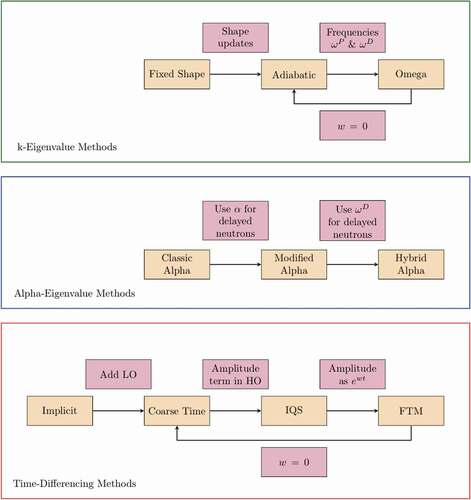
Figure 6 encapsulates the differences and similarities between methods in a single illustration.

Fig. 6. Summary of HOLO methods and their relationships.

III. RESULTS

Results obtained with the methods described will now be compared against each other. We expect the error of the eigenvalue methods to be worse than the time-differencing methods, which is supported by the results. Different eigenvalue methods will be compared against each other and likewise for the time-differencing methods. The reference solution in all cases is the fully implicit method with time steps of 10⁻⁵ s and no low-order method. PKEs will use inner time steps of 10⁻⁴ s, which showed no difference with 10⁻⁵ s or 10⁻⁶ s. A variety of outer time step sizes are tested to observe the convergence behavior of each method.

All methods use the same 1 cm mesh and the same convergence criterion of 10⁻¹⁰ for calculating flux. All methods employ a linear shape interpolation whereby the outer time steps are calculated twice to improve the interpolation of point kinetics parameters. Thanks to this, a full spatial precursor distribution can be computed at every inner time step, regardless of the method. This implies that when a $C^{n+1}$ term is used, it includes full spatial resolution.

III.A. Eigenvalue Methods

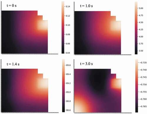
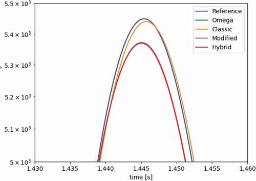
The fixed shape method is quickly determined to be erroneous by comparing the transient’s power profile in Fig. 7, where all curves are nearly overlapping except for the fixed shape method. This stresses the importance of flux shape updates. The error of the adiabatic and omega methods is more subtle. Figure 8 provides a close-up of the peak to visualize the differences. We look at the values of k-balance in Fig. 9 to determine the impact of frequencies in the omega method. If the frequencies are accurate, k-balance should be exactly 1. For the adiabatic method, on the other hand, we expect the change in k to follow the reactivity change of the problem. Figure 9 confirms both. Figures 10 and 11 show the evolution of the prompt and delayed frequencies throughout the transient. Figure 12 shows the spatial resolution of the delayed frequencies as the transient evolves. All these behave as expected.

Fig. 7. Power profile shows that the fixed shape method is inadequate.

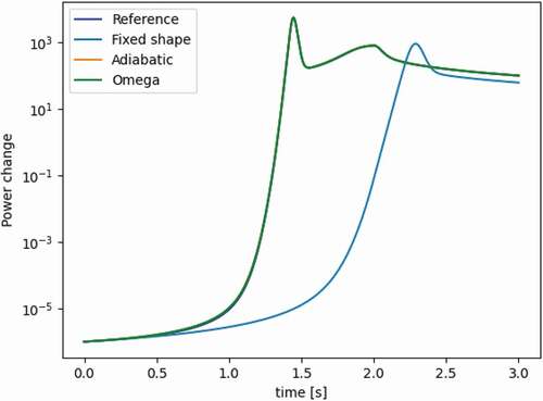
Fig. 8. Zoom-in to the first peak.

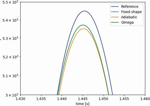
Fig. 9. Values of k-balance over time.

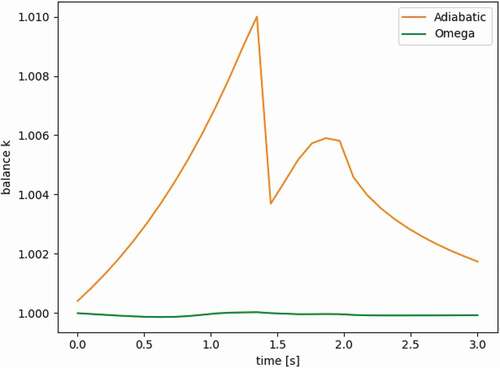
Fig. 10. Prompt frequencies as calculated by the omega method (in units of inverse seconds).

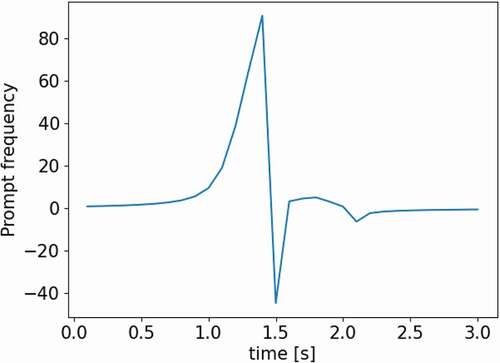
Fig. 11. Precursor frequencies for each delayed neutron group in the first cell of the geometry as calculated by the omega method (in units of inverse seconds).

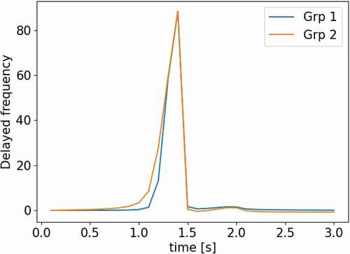
Fig. 12. Spatial distribution of delayed frequencies for precursor group 2 at different points in time, as calculated by the omega method (in units of inverse seconds).

The results in Tables II and III highlight that the omega method is better than the adiabatic method for predicting the transient peak. Errors fluctuate, sometimes improving, sometimes degrading with refined time steps. This suggests that a convergence plateau has been reached, likely at 0.1 s. The eigenvalue methods introduce an underlying error by assuming that a static update of the shape can characterize the transient. This inherently flawed approach prohibits the solution from converging to the correct answer, even at fine time steps. Results in Figs. 7 through 12 are shown for outer time steps of 0.1 s.

TABLE II Sensitivity of the Adiabatic Method to Outer Time Step Size

	Reference	0.01 s Outer Step Solution	0.01 s	0.05 s	0.1 s	0.5 s
			Percent Relative Difference from Reference
Time to first peak (s)	1.44545	1.4453	0.01	0.00	0.02	0.13
Power at first peak (W/cm^3)	5448.7	5338.6	2.02	1.37	1.80	0.41
Power at second peak (W/cm^3)	792.8	790.4	0.30	0.26	0.19	1.12
Power at t = 3 s (W/cm^3)	98.06	98.79	0.74	0.75	0.69	0.58

TABLE III Sensitivity of the Omega Method to Outer Time Step Size

	Reference	0.01 s Outer Step Solution	0.01 s	0.05 s	0.1 s	0.5 s
			Percent Relative Difference from Reference
Time to first peak (s)	1.44545	1.4452	0.02	0.02	0.02	0.16
Power at first peak (W/cm^3)	5448.7	5364.5	1.55	1.11	1.43	0.01
Power at second peak (W/cm^3)	792.8	792.2	0.08	0.06	0.04	1.01
Power at t = 3 s (W/cm^3)	98.06	98.90	0.86	0.87	0.84	0.61

The omega method is expected to have better spatial resolution because of the spatially dependent precursor frequencies. Figure 13 compares the shape of the assembly powers at the power peak. The omega method is confirmed to outperform the adiabatic method in this respect, with a 22% lower power error root-mean-square (RMS) for omega. Figure 14 compares the end-of-transient temperatures, which illustrates the cumulative effect of the power change during the transient. The region of the control rod movement has lower error with the omega method, but that is not true of the rest of the reactor. This suggests that the exponential frequencies work best in the extreme parts of the transient that can be characterized by an exponential change.

Fig. 13. Normalized assembly power densities at the peak for adiabatic versus omega. In green and red are errors that are lower and higher for omega method, respectively.

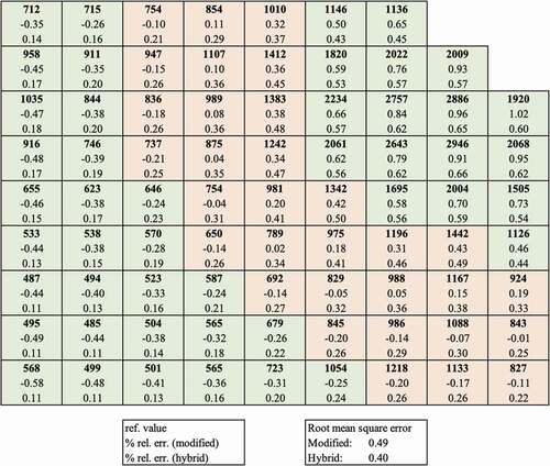
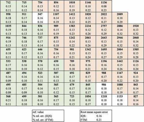
Fig. 14. Assembly temperatures at the end of transient for adiabatic versus omega. In green and red are errors that are lower and higher for omega method, respectively.

Next, we compare alpha-eigenvalue methods to the omega method. The classic alpha method is implemented for illustration: Although the start of the transient is well simulated in the absence of delayed neutron modeling, the peak is significantly different from the omega method and the other alpha-eigenvalue methods as seen in Fig. 15. The fact that it is very close to the reference solution is likely a coincidence. Table IV emphasizes that although the power at the first peak happens to be very accurate, the power at the second peak and at 3 s is significantly worse for the classic alpha-eigenvalue method.

TABLE IV Alpha Eigenvalue Results, Obtained with 0.1 s Outer Time Steps

	Reference	Classic	Modified	Hybrid
		Percent Relative Difference from Reference
Time to first peak (s)	1.44545	0.02	0.02	0.02
Power at first peak (W/cm^3)	5448.7	0.16	1.47	1.42
Power at second peak (W/cm^3)	792.8	0.98	0.29	0.05
Power at t = 3 s (W/cm^3)	98.06	1.78	0.50	0.84

Fig. 15. Power profile, zoomed-in.

The modified alpha method is a simple way to include delayed neutrons into the classic alpha-eigenvalue method. The hybrid alpha method is more sophisticated and includes spatial resolution. Figures 16 and 17 show that hybrid alpha is an improvement over modified alpha. Hybrid alpha even appears to outperform the omega method. The only difference between the omega and hybrid alpha methods is the prompt frequency. The omega method calculates a prompt frequency from the inner steps whereas hybrid alpha uses the critical search algorithm to determine alpha. This suggests that the alpha-eigenvalue search method is more robust than the prompt frequency calculation, although it is significantly more expensive because of the iterative methodology used to evaluate alpha. In Fig. 18, the power distribution at the peak clearly shows that the hybrid alpha method has better spatial resolution than the modified alpha method, as expected. The power error RMS is 17% lower for hybrid. In Fig. 19, the end-of-transient temperatures show a similar trend to the adiabatic and omega methods but less pronounced. In other words, the hybrid alpha method is a larger improvement on the modified alpha than omega is on adiabatic.

Fig. 16. Absolute error with respect to reference, in time, zoomed to the second peak.

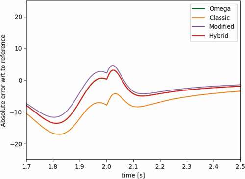
Fig. 17. Values of k-balance over time.

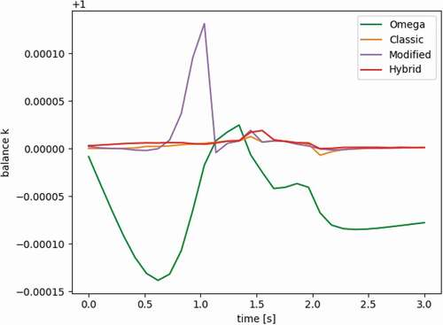
Fig. 18. Normalized assembly power densities at the peak for modified versus hybrid alpha. In green and red are errors that are lower or higher for hybrid, respectively.

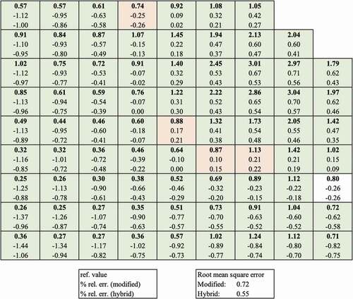
Fig. 19. Assembly temperatures at the end of transient for modified versus hybrid alpha. In green and red are errors that are lower or higher for hybrid, respectively.

III.B. Time-Differencing Methods

We now compare the coarse time integration, the IQS method, and the FTM against each other. Finer time steps are required for stability as discussed earlier. Table V assesses the temporal convergence of the coarse time-differencing method. We notice that it does not converge linearly the way the implicit method does. This is due to the effect of PKEs and linear shape interpolation between outer time steps. To prove this, we provide Table VI, a temporal convergence analysis of a “stripped down” version of the coarse time integration. This “strip down” includes removing linear interpolation and using lagging Doppler feedback, as opposed to the PKE-calculated values. By removing these elements, the PKE contributions are deleted, and the method retains only the time-differencing between outer steps. As seen in Table VI, the method now approaches linear convergence. Therefore, the addition of a low-order method impacts the temporal convergence properties of the high-order method but provides greater accuracy as the outer time steps are lengthened. Notice that the error of the stripped-down method at time steps of 10⁻³ s is similar to the implicit method. The addition of the low-order method allows the error to be reduced as the time steps get larger. Results in Table VII and all figures in this section are shown for outer time steps of 0.01 s.

TABLE V Sensitivity of the Coarse Time Integration Method to Outer Time Step Size

	Reference	0.001 s Outer Step Solution	0.001 s	0.005 s	0.01 s
			Percent Relative Difference from Reference
Time to first peak (s)	1.44545	1.4457	0.02	0.01	0.02
Power at first peak (W/cm^3)	5448.7	5389.9	1.08	1.20	1.55
Power at second peak (W/cm^3)	792.8	791.2	0.20	0.21	0.24
Power at t = 3 s (W/cm^3)	98.06	98.27	0.21	0.21	0.21

TABLE VI Sensitivity of the Stripped-Down Coarse Time Integration Method to Outer Time Step Size

	Reference	0.001 s Outer Step Solution	0.001 s	0.005 s	0.01 s
			Percent Relative Difference from Reference
Time to first peak (s)	1.44545	1.440	0.38	2.11	4.53
Power at first peak (W/cm^3)	5448.7	5425.1	0.43	2.03	3.56
Power at second peak (W/cm^3)	792.8	794.0	0.15	0.45	0.10
Power at t = 3 s (W/cm^3)	98.06	98.01	0.05	0.25	0.50

TABLE VII Time-Differencing Results, Obtained with 0.01 s Outer Time Steps

	Reference	Coarse	IQS	FTM
		Percent Relative Difference from Reference
Time to first peak (s)	1.44545	0.02	0.14	0.09
Power at first peak (W/cm^3)	5448.7	1.55	1.58	0.94
Power at second peak (W/cm^3)	792.8	0.24	0.16	0.32
Power at t = 3 s (W/cm^3)	98.06	0.21	0.10	0.13

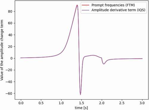
The FTM employs frequencies, and the IQS method employs amplitude derivatives, but both serve a similar purpose to approximate the amplitude change. These amplitude change terms were computed as instantaneous values based on the two most recent inner time steps. Figure 20 emphasizes the similarity of these terms, as their values overlap throughout the transient. It is conjectured therefore that the differences between the IQS method and the FTM results are mainly due to the formulation of the precursor equations, which is the major difference between the two methods. While the IQS method performs a numerical precursor integration, the FTM solves for the precursors analytically, as detailed in Sec. II.D.3.

Fig. 20. Comparing prompt frequencies in the FTM to the amplitude derivative term in the IQS method.

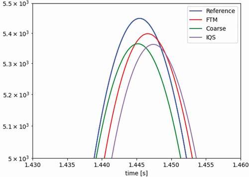
From Fig. 21 and Table VII, the FTM predicts the time and power of the peak better, but the IQS method performs better later in the transient.

Fig. 21. Zoomed-in power profile.

We next look at the spatial error. The FTM has a more accurate power distribution at the peak as shown in Fig. 22 with a RMS error of 27% lower for the FTM. For end-of-transient temperatures, the methods are more similar as shown in Fig. 23. In general, the IQS method and the FTM appear to have much in common. The precursor concentration calculation, which is the main difference between the two methods, carries much of the spatial distribution of the problem. Therefore, our conjecture about the use of a numerical precursor integration versus an analytic solution being the primary difference between the two methods is reinforced.

Fig. 22. Normalized assembly power densities at the peak for the IQS method versus the FTM. In green and red are errors that are lower and higher for FTM, respectively.

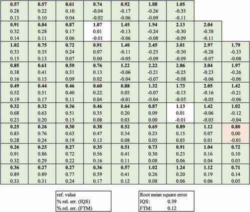
Fig. 23. Assembly temperatures at the end of transient for the IQS method versus the FTM. In green and red are errors that are lower and higher for FTM, respectively.

IV. CONCLUSIONS AND APPLICATIONS

Three categories of HOLO methods, specifically for transient analysis, were directly compared on a common benchmark for the first time.

In the category of k-eigenvalue methods, the fixed shape method illustrated the strong need for flux shape calculations throughout transient simulations. The errors associated with the adiabatic method and the omega method were analyzed to conclude that the omega method is more accurate thanks to the presence of a prompt frequency and spatially distributed precursor frequencies, increasing the spatial resolution of the transient through the frequency transform, which assumes exponential behavior.

For alpha-eigenvalue methods, two alternatives to the classic alpha-eigenvalue method were developed and tested. The hybrid alpha mode was much more effective than the modified alpha mode. We recommend using this hybrid mode for all alpha-eigenvalue simulations of reactor transients. The hybrid alpha-eigenvalue method even outperformed the omega method, although at a greater expense.

Finally, for time-differencing schemes, the coarse time integration was the least favorable method because it ignores the derivative of the amplitude when updating the flux shape. By adding frequencies, the coarse time integration method becomes the FTM, which showed large improvements. The IQS method and the FTM showed many similarities, especially in the behavior of the amplitude derivative terms. In fact, the IQS method can be considered a generalized form of the FTM. The relative accuracy of the IQS method compared to the FTM appears to be strongly problem dependent: If the power change cannot be characterized as exponential, the more general IQS method is recommended thanks to its flexibility. However, during exponential transients, the FTM is recommended for better precursor accuracy and therefore spatial resolution.

Overall, the use of exponential frequencies, especially spatially distributed precursor frequencies, has the largest impact in improving transient simulation accuracy when using HOLO methods. The RMS error in power distribution at the peak was consistently about 20% lower when using frequencies, as emphasized in Table VIII. These frequencies allow for two-way communication between the high-order and the low-order solvers. These results corroborate similar findings in high-fidelity scenarios where the omega method was shown to be more spatially accurate than the adiabatic method in a Monte Carlo/coarse mesh finite difference coupling scheme.⁹

TABLE VIII Impact of Frequencies on Peak Power RMS Error

	RMS Error in Absence of Frequencies	RMS Error in Presence of Frequencies	Difference in RMS Error
k-eigenvalue methods	Adiabatic	Omega	22%
	0.79	0.57
Alpha-eigenvalue methods	Modified alpha	Hybrid alpha	17%
	0.72	0.55
Time-differencing methods	IQS	FTM	27%
	0.39	0.12

The results of this work confirm the expected behavior of the methods presented for the 2D-LRA benchmark. Further work could be done to assess their accuracy in different power change regimes. For instance, if the power change is not exponential, then the use of exponential frequencies is not expected to be as robust.

Nomenclature

$C_i$	=	= group i delayed neutron precursor concentration
$D_g$	=	= group g diffusion coefficient
$k$	=	= neutron multiplication factor
$k_{crit}$	=	= neutron multiplication factor in the initial reactor state
$P$	=	= power
$S_g$	=	= group g source term
$T$	=	= temperature
$t$	=	= time
$v_g$	=	= group g neutron velocity
$\vec{x}$	=	= space

Greek

$\alpha$	=	= alpha eigenvalue
$\theta$	=	= temperature conversion factor
${\beta }_i$	=	= group i delayed neutron fraction
$\gamma$	=	= Doppler feedback coefficient
$\mathrm{\Delta }t$	=	= time step
$\kappa$	=	= thermal energy per fission
$\mathrm{\Lambda }$	=	= prompt neutron lifetime
${\lambda }_i$	=	= group i decay constant
${\nu }_g$	=	= group g fission yield
$\rho$	=	= reactivity
${\mathrm{\Sigma }}_{a,g}$	=	= group g macroscopic absorption cross section
${\mathrm{\Sigma }}_{a,g,R}$	=	= group g macroscopic absorption cross section in region R
${\mathrm{\Sigma }}_{f,g}$	=	= group g macroscopic fission cross section
${\mathrm{\Sigma }}_{r,g}$	=	= group g macroscopic removal cross section
${\mathrm{\Sigma }}_{s,g{ }^{\mathrm{\prime }}\to g}$	=	= group g macroscopic in-scatter cross section
${\varphi }_g$	=	= group g neutron flux shape amplitude
${\chi }_g^D$	=	= delayed fission neutron spectrum
${\chi }_g^{eq}$	=	= equilibrium fission neutron spectrum
${\chi }_g^P$	=	= prompt fission neutron spectrum
${\mathrm{\Psi }}_g$	=	= group g neutron flux
${\psi }_g$	=	= group g neutron flux shape
${\psi }_g^{\ast }$	=	= group g neutron adjoint flux shape
${\omega }^{D,i}$	=	= group i delayed frequency
${\omega }^{P,g}$	=	= group g prompt frequency

Acknowledgments

The first author was funded by the U.S. Department of Energy (DOE) Computational Science Graduate Fellowship under grant DE-FG02-97ER25308. This research was also partially supported by the Exascale Computing Project (17-SC-20-SC), a collaborative effort of the DOE Office of Science and the National Nuclear Security Administration.

APPENDIX A

DESCRIPTION OF THE 2D-LRA TRANSIENT BENCHMARK

The benchmark includes data for two energy groups and data for two delayed neutron precursor groups. Regions 1, 2, 3, and 4 in Fig. A.1 are fuel regions with different cross sections. The rod withdrawal is modeled by a linear reduction in the thermal absorption cross section in region R for the first 2 s of the transient [see Eq. (A.1)(34) $\begin{array}{rl}& -\mathrm{\nabla }\cdot D_g^{n+1}\mathrm{\nabla }{\psi }_g^{n+1}+\left[{\mathrm{\Sigma }}_{rg}^{n+1}+\frac{\omega }{v_g}+\frac{1}{v_g\mathrm{\Delta }t}\right]{\psi }_g^{n+1}\\ & -\sum _{g^{\prime }\ne g}{\mathrm{\Sigma }}_{s{g}^{\prime }\to g}^{n+1}{\psi }_g^{n+1}-\left[\left(1-{\beta }_{tot}\right)\frac{{\chi }_g^P}{k_{crit}}\right.\\ & \left.+\sum _i{\chi }_g^D{\lambda }_i\frac{{\beta }_i}{k_{crit}\left({\lambda }_i+\omega \right)}\left(1-\frac{1-e^{-\left({\lambda }_i+\omega \right)\mathrm{\Delta }t}}{\left({\lambda }_i+\omega \right)\mathrm{\Delta }t}\right)\right]\\ & \sum _{g^{\prime }}{\nu }_{g^{\prime }}{\mathrm{\Sigma }}_{f{g}^{\prime }}^{n+1}{\psi }_{g^{\prime }}^{n+1}=\sum _i{\chi }_g^D{\lambda }_i\frac{{\beta }_i}{k_{crit}\left({\lambda }_i+\omega \right)}\\ & \left(-e^{-\left({\lambda }_i+\omega \right)\mathrm{\Delta }t}+\frac{1-e^{-\left({\lambda }_i+\omega \right)\mathrm{\Delta }t}}{\left({\lambda }_i+\omega \right)\mathrm{\Delta }t}\right)\sum _{g^{\prime }}{\nu }_{g^{\prime }}{\mathrm{\Sigma }}_{f{g}^{\prime }}^{n+1}{\psi }_{g^{\prime }}^n\\ & +\sum _i{\chi }_g^D{\lambda }_i{C}_i^n{e}^{-\left({\lambda }_i+\omega \right)\mathrm{\Delta }t}+\frac{{\psi }_g^n}{v_g\mathrm{\Delta }t}.\end{array}$(34) ]. Adiabatic heatup is modeled based on the change in temperature and power [see Eqs. (A.2)(35) $\begin{array}{c}\left\{\begin{array}{c}-\mathrm{\nabla }\cdot D_1^{n+1}\mathrm{\nabla }{\psi }_1^{n+1}+\widehat{{\mathrm{\Sigma }}_{r1}^{n+1}}{\psi }_1^{n+1}-\sum _{g{ }^{\mathrm{\prime }}}\stackrel{ˆ}{{\mathrm{\Sigma }}_{fg{ }^{\mathrm{\prime }}}^{n+1}}{\psi }_{g{ }^{\mathrm{\prime }}}^{n+1}=S_1\\ -\mathrm{\nabla }\cdot D_2^{n+1}\mathrm{\nabla }{\psi }_2^{n+1}+\widehat{{\mathrm{\Sigma }}_{r2}^{n+1}}{\psi }_2^{n+1}-{\mathrm{\Sigma }}_{s1\to 2}^{n+1}{\psi }_1^{n+1}=S_2\end{array}\right..\end{array}$(35) and (A.3)(A.1) ${\Sigma }_{a2,R}\left(t\right)=\{{\Sigma }_{a2,3}^0\cdot \left(1-\left[0.0606184\cdot t\right]\right)\text{if}t\le 2s{\Sigma }_{a2,3}^0\cdot \left(1-\left[0.0606184\cdot 2\right]\right)\text{if}t2s.$(A.1) ]. Doppler feedback is simulated as a change in fast absorption cross section in all fuel regions [see Eq. (A.4)(A.2) $\frac{\partial T\left(t,\overrightarrow{x}\right)}{\partial t}=\theta \sum g\prime =12\Sigma fg\prime \Psi g\prime \left(t,\overrightarrow{x}\right)$(A.2) ]. The two inner sides of the geometry have reflective boundary conditions, and the two outer sides of the core have zero flux boundary conditions.

The rod withdrawal is prescribed as

(A.1) ${\Sigma }_{a2,R}\left(t\right)=\{{\Sigma }_{a2,3}^0\cdot \left(1-\left[0.0606184\cdot t\right]\right)\text{if}t\le 2s{\Sigma }_{a2,3}^0\cdot \left(1-\left[0.0606184\cdot 2\right]\right)\text{if}t2s.$(A.1)

The adiabatic heatup and power equations are

(A.2) $\frac{\partial T\left(t,\overrightarrow{x}\right)}{\partial t}=\theta \sum g\prime =12\Sigma fg\prime \Psi g\prime \left(t,\overrightarrow{x}\right)$(A.2)

and

(A.3) $\begin{array}{c}P\left(t,\vec{x}\right)=\kappa \sum _{g{ }^{\mathrm{\prime }}=1}^2{\mathrm{\Sigma }}_{fg{ }^{\mathrm{\prime }}}{\mathrm{\Psi }}_{g{ }^{\mathrm{\prime }}}\left(t,\vec{x}\right).\end{array}$(A.3)

The Doppler feedback is modeled as

(A.4) $\begin{array}{c}{\mathrm{\Sigma }}_{a,1}\left(T\right)={\mathrm{\Sigma }}_{a1}^0\left[1+\gamma \left(\sqrt{T}-\sqrt{T^0}\right)\right],\end{array}$(A.4)

where $\theta ,\kappa ,\mathrm{a}\mathrm{n}\mathrm{d}\gamma$ are specified in the benchmark along with other relevant reactor-wide parameters. Note that most published solutions use a slightly modified benchmark whereby the Doppler feedback coefficient $\gamma$ is 3.034 × 10⁻³ K^−1/2 (instead of 2.034 × 10⁻³ K^−1/2) and the decay constant for the first delayed neutron precursor group is 0.0654 s⁻¹ (instead of 0.00654 s⁻¹) (Ref. 27). These modified values are used in this paper for consistency with other published results.

Fig. A.1. 2D-LRA geometry.¹¹

APPENDIX B

DETAILED DERIVATION OF THE ANALYTIC PRECURSOR SOLUTION FOR THE FTM

The only assumption in the analytical solution to the precursor equation is that the time variation of the flux shape is linear over the time step

(B.1) $\frac{d{C}_i\left(t\right)}{dt}=-{\lambda }_i{C}_i\left(t\right)+e^{\omega t}\frac{{\beta }_i}{k_{crit}}{\displaystyle \sum _{g^{\prime }}{\nu }_{g^{\prime }}}{\Sigma }_{f{g}^{\prime }}{\psi }_{g^{\prime }}\left(t\right)$(B.1)

and

(B.2) $\psi \left(t\right)={\psi }^n+\frac{t-t^n}{\Delta t}\left[{\psi }^{n+1}-{\psi }^n\right].$(B.2)

Substituting the linear shape assumption into the precursor equation with $t^n=0,$

(B.3) $\begin{array}{rl}& \frac{d{C}_i\left(t\right)}{dt}=-{\lambda }_i{C}_i\left(t\right)+e^{\omega t}\frac{{\beta }_i}{k_{crit}}\\ & \sum _{g^{\prime }}{\nu }_{g^{\prime }}{\mathrm{\Sigma }}_{f{g}^{\prime }}\left[{\psi }_{g^{\prime }}^n+t\frac{{\psi }_{g^{\prime }}^{n+1}-{\psi }_{g^{\prime }}^n}{\mathrm{\Delta }t}\right].& (\mathrm{B}.3)\end{array}$(B.3)

Grouping terms together into intermediate variables a and b for readability,

(B.4) $\begin{array}{rl}& \frac{d{C}_i\left(t\right)}{dt}=-{\lambda }_i{C}_i\left(t\right)+e^{\omega t}\frac{{\beta }_{\mathit{i}}}{{\mathit{k}}_{\mathit{c}\mathit{r}\mathit{i}\mathit{t}}}\sum _{{\mathit{g}}^{\prime }}{\nu }_{{\mathit{g}}^{\prime }}{\mathrm{\Sigma }}_{{\mathit{f}\mathit{g}}^{\prime }}{\psi }_{{\mathit{g}}^{\prime }}^{\mathit{n}}+t{e}^{\omega t}\frac{{\beta }_{\mathbf{i}}}{{\mathit{k}}_{\mathit{c}\mathit{r}\mathit{i}\mathit{t}}}\sum _{{\mathit{g}}^{\prime }}{\nu }_{{\mathit{g}}^{\prime }}{\mathrm{\Sigma }}_{{\mathit{f}\mathit{g}}^{\prime }}\left[\frac{{\psi }_{{\mathit{g}}^{\prime }}^{\mathit{n}+\mathbf{1}}-{\psi }_{{\mathit{g}}^{\prime }}^{\mathit{n}}}{\mathrm{\Delta }\mathit{t}}\right]\end{array}$(B.4)

becomes

(B.5) $\begin{array}{c}{C}_i^{\prime }\left(t\right)=-{\lambda }_i{C}_i\left(t\right)+\mathit{a}{e}^{\omega t}+\mathit{b}t{e}^{\omega t}.\end{array}$(B.5)

Solving this ordinary differential equation with the initial condition $C_i\left(0\right)=C_i^n,$

(B.6) $C_i\left(t\right)=C_i^n{e}^{-{\lambda }_{i}t}+\frac{e^{-{\lambda }_{i}t}}{{\lambda }_i+\omega }\left[a{e}^{\left({\lambda }_i+\omega \right)t}-a+bt{e}^{\left({\lambda }_i+\omega \right)t}-b\frac{e^{\left({\lambda }_i+\omega \right)t}}{{\lambda }_i+\omega }+\frac{b}{{\lambda }_i+\omega }\right].$(B.6)

Replacing a and b with their original expressions, factoring out the common terms (${\beta }_i/k_{crit},{\nu }_g{\mathrm{\Sigma }}_{fg}$),

(B.7) $\begin{array}{rl}& C_i(t)+{C_i}^n{e}^{-{\lambda }_{i}t}+\frac{{\beta }_i{e}^{-{\lambda }_{i}t}}{k_{crit}({\lambda }_i+\omega )}\sum _{g^{\prime }\hspace{0.17em}}{\nu }_{g^{\prime }\hspace{0.17em}}{\mathrm{\Sigma }}_{f{g}^{\prime }\hspace{0.17em}}\\ & \left[{\psi }_{g\prime }^n{e}^{({\lambda }_i+\omega )t}-{\psi }_{g\prime \hspace{0.17em}}^n+\frac{{\psi }_{g\prime \hspace{0.17em}}^{n+1}-{\psi }_{g\prime \hspace{0.17em}}^n}{\mathrm{\Delta }t}t{e}^{({\lambda }_i+\omega )t}-\frac{{\psi }_{g\prime \hspace{0.17em}}^{n+1}-{\psi }_{g\prime \hspace{0.17em}}^n}{\mathrm{\Delta }t}\frac{e^{({\lambda }_i+\omega )t}}{{\lambda }_i+\omega }+\frac{{\psi }_{g\prime \hspace{0.17em}}^{n+1}-{\psi }_{g\prime \hspace{0.17em}}^n}{\mathrm{\Delta }t}\frac{1}{{\lambda }_i+\omega }\right].& (\mathrm{B}.7)\end{array}$(B.7)

Grouping together terms multiplied by ${\psi }_g^n$ and ${\psi }_g^{n+1},$ respectively,

(B.8) $\begin{array}{rl}& C_i\left(t\right)=C_i^n{e}^{-{\lambda }_{i}t}+\frac{{\beta }_i{e}^{-{\lambda }_{i}t}}{k_{crit}({\lambda }_i+\omega )}\sum _{g^{\prime }}{\nu }_{g^{\prime }}{\mathrm{\Sigma }}_{f{g}^{\prime }}\left[{\psi }_{g^{\prime }}^n\left(e^{({\lambda }_i+\omega )t}-1-\frac{t}{\mathrm{\Delta }t}{e}^{({\lambda }_i+\omega )t}+\frac{e^{({\lambda }_i+\omega )t}}{({\lambda }_i+\omega )\mathrm{\Delta }t}-\frac{1}{({\lambda }_i+\omega )\mathrm{\Delta }t}\right)\right.\\ & \left.+{\psi }_{g^{\prime }}^{n+1}\left(\frac{t{e}^{({\lambda }_i+\omega )t}}{\mathrm{\Delta }t}-\frac{e^{({\lambda }_i+\omega )t}}{({\lambda }_i+\omega )\mathrm{\Delta }t}+\frac{1}{({\lambda }_i+\omega )\mathrm{\Delta }t}\right)\right].& (\mathrm{B}.8)\end{array}$(B.8)

Multiplying through by $\frac{e^{\left({\lambda }_i+\omega \right)t}}{e^{\left({\lambda }_i+\omega \right)t}}$ to transform $e^{-{\lambda }_{i}t}$ into $e^{\omega t}$ as the common factor of the second term,

(B.9) $\begin{array}{rl}& C_i\left(t\right)=C_i^n{e}^{-{\lambda }_{i}t}+\frac{{\beta }_i{e}^{\omega t}}{k_{crit}({\lambda }_i+\omega )}\sum _{g^{\prime }}{{\nu }_g}^{\prime }\sum f{g}^{\prime }\\ & \left[{\psi }_{g^{\prime }}^n\left(1-e^{-({\lambda }_i+\omega )t}-\frac{t}{\mathrm{\Delta }t}+\frac{1}{({\lambda }_i+\omega )\mathrm{\Delta }t}-\frac{e^{-({\lambda }_i+\omega )t}}{({\lambda }_i+\omega )\mathrm{\Delta }t}\right)+{\psi }_{g^{\prime }}^{n+1}\left(\frac{t}{\mathrm{\Delta }t}-\frac{1}{({\lambda }_i+\omega )\mathrm{\Delta }t}+\frac{e^{-({\lambda }_i+\omega )t}}{({\lambda }_i+\omega )\mathrm{\Delta }t}\right)\right].& (\mathrm{B}.9)\end{array}$(B.9)

Evaluating the expression at $C_i\left(\mathrm{\Delta }t\right)=C^{n+1},$

(B.10) $C_i{ }^{n+1}=C_i^n{e}^{-{\lambda }_i\Delta t}+\frac{{\beta }_i{e}^{\omega \Delta t}}{k_{crit}({\lambda }_i+\omega )}{\displaystyle \sum _{g^{\prime }}{\nu }_{g^{\prime }}}{\displaystyle {\sum }_{f{g}^{\prime }} }\left[{\psi }_{g^{\prime }}^n\left(1-e^{-({\lambda }_i+\omega )\Delta t}-1+\frac{1}{({\lambda }_i+\omega )\Delta t}-\frac{e^{-({\lambda }_i+\omega )t}}{({\lambda }_i+\omega )\Delta t}\right)+{\psi }_{g^{\prime }}^{n+1}\left(1-\frac{1}{({\lambda }_i+\omega )\Delta t}+\frac{e^{-({\lambda }_i+\omega )t}}{({\lambda }_i+\omega )\Delta t}\right)\right].(\text{B}.\text{10})$(B.10)

Rearranging terms,

(B.11) $\begin{array}{rl}& C_i^{n+1}=C_i^n{e}^{-{\lambda }_i\mathrm{\Delta }t}+\frac{{\beta }_i{e}^{\omega \mathrm{\Delta }t}}{k_{crit}\left({\lambda }_i+\omega \right)}\sum _{g^{\prime }}{\nu }_{g^{\prime }}{\mathrm{\Sigma }}_{f{g}^{\prime }}\left[{\psi }_{g^{\prime }}^n\left(-e^{-\left({\lambda }_i+\omega \right)\mathrm{\Delta }t}+\frac{1-e^{-\left({\lambda }_i+\omega \right)\mathrm{\Delta }t}}{\left({\lambda }_i+\omega \right)\mathrm{\Delta }t}\right)+{\psi }_{g^{\prime }}^{n+1}\left(1-\frac{1-e^{-\left({\lambda }_i+\omega \right)\mathrm{\Delta }t}}{\left({\lambda }_i+\omega \right)\mathrm{\Delta }t}\right)\hspace{0.17em}\right].(\mathrm{B}.11)\end{array}$(B.11)

References

- B. SJENITZER and J. HOOGENBOOM, “General Purpose Dynamic Monte Carlo with Continuous Energy for Transient Analysis,” Proc. PHYSOR 2012, Knoxville, Tennessee, April 15–20, 2012, American Nuclear Society (2012).
- V. VALTAVIRTA, M. HESSAN, and J. LEPPÄNEN, “Delayed Neutron Emission Model for Time Dependent Simulations with the SERPENT 2 Monte Carlo Code—First Results,” Proc. PHYSOR 2016, Sun Valley, Idaho, May 1–5, 2016, American Nuclear Society (2016).
- D. FERRARO et al., “SERPENT and TRIPOLI-4 Transient Calculations Comparisons for Several Reactivity Insertion Scenarios in a 3D Minicore Benchmark,” Proc. Int. Conf. Mathematics and Computational Methods Applied to Nuclear Science and Engineering (M&C 2019), Portland, Oregon, August 25–29, 2019, American Nuclear Society (2019).
- L. LI, “A Low Order Acceleration Scheme for Solving the Neutron Transport Equation,” PhD Thesis, Massachusetts Institute of Technology, Nuclear Science & Engineering (2013).
- L. JAIN, R. KARTHIKEYAN, and U. KANNAN, “Multi-Grid Acceleration Scheme for Neutron Transport Calculations Using Optimally Diffusion CMFD Method,” Proc. Symp. Advanced Sensors and Modeling Techniques for Nuclear Reactor Safety, Bombay, India, December 15–19, 2018.
- B. CHANG et al., “Spatial Multigrid for Isotropic Neutron Transport,” SIAM J. Sci. Comput., 29, 5, 1900 (2007); https://doi.org/https://doi.org/10.1137/060661363.
- J. YOON and H. JOO, “Two-Level Coarse Mesh Finite Difference Formulation with Multigroup Source Expansion Nodal Kernels,” J. Nucl. Sci. Technol., 45, 7, 668 (2008); https://doi.org/https://doi.org/10.1080/18811248.2008.9711467.
- C. BENTLEY, “Improvements in a Hybrid Stochastic/Deterministic Method for Transient Three-Dimensional Neutron Transport,” PhD Thesis, University of Tennessee Knoxville, Nuclear Engineering (1996).
- S. SHANER, “Development of High Fidelity Methods for 3D Monte Carlo Analysis of Nuclear Reactors,” PhD Thesis, Massachusetts Institute of Technology, Nuclear Science & Engineering (2018).
- BENCHMARK PROBLEM COMMITTEE, “Argonne Code Center: Benchmark Problem Book,” ANL-7416 and Suppl. 2, Argonne National Laboratory (1977).
- M. ABDO, R. ELZOHERY, and J. ROBERT, “Analysis of the LRA Reactor Benchmark Using Dynamic Mode Decomposition,” Trans. Am. Nucl. Soc., 119, 683 (2018).
- K. SMITH, “An Analytical Nodal Method for Solving the Two Group, Multidimensional, Static and Transient Neutron Diffusion Equation,” Master Thesis, Massachusetts Institute of Technology, Nuclear Science & Engineering (1979).
- J. BANFIELD, “Semi-Implicit Direct Kinetics Methodology for Deterministic, Time-Dependent, Three-Dimensional, and Fine-Energy Neutron Transport Solutions,” PhD Thesis, University of Tennessee Knoxville, Nuclear Engineering (2013).
- B. BANDINI, “A Three-Dimensional Transient Neutronics Routine for the TRAC-PF1 Reactor Thermal Hydraulic Computer Code,” PhD Thesis, The Pennsylvania State University, Nuclear Engineering (1990).
- Q. WU et al., “Whole-Core Forward-Adjoint Neutron Transport Solutions with Coupled 2-D MOC and 1-D SN and Kinetics Parameter Calculation,” Prog. Nucl. Energy, 108, 310 (2018); https://doi.org/https://doi.org/10.1016/j.pnucene.2018.06.006.
- J. YASINSKY and A. HENRY, “Some Numerical Experiments Concerning Space-Time Reactor Kinetics Behavior,” Nucl. Sci. Eng., 22, 2, 171 (1965); https://doi.org/https://doi.org/10.13182/NSE65-A20236.
- Z. PRINCE and J. RAGUSA, “Multiphysics Reactor-Core Simulations Using the Improved Quasi-Static Method,” Ann. Nucl. Energy, 125, 186 (2019); https://doi.org/https://doi.org/10.1016/j.anucene.2018.10.056.
- A. AL-MOHY and N. HIGHAM, “A New Scaling and Squaring Algorithm for the Matrix Exponential,” SIAM J. Matrix Anal. Appl., 31, 3, 970 (2009); https://doi.org/https://doi.org/10.1137/09074721X.
- D. FERGUSON and K. HANSEN, “Solution of the Space-Dependent Reactor Kinetics Equations in Three Dimensions,” MIT-2903-4, U.S. Atomic Energy Commission (1971).
- M. ORTEGA, “A Rayleigh Quotient Fixed Point Method for Criticality Eigenvalue Problems in Neutron Transport,” PhD Thesis, University of California Berkeley, Nuclear Engineering (2019).
- T. HILL, “Efficient Methods for Time Absorption (α) Eigenvalue Calculations,” LA-9602-MS, Los Alamos National Laboratory (1983).
- C. JOSEY and F. BROWN, “A New Monte Carlo Alpha-Eigenvalue Estimator with Delayed Neutrons,” Trans. Am. Nucl. Soc., 118, 903 (2018).
- K. OTT and D. MENELEY, “Accuracy of the Quasistatic Treatment of Spatial Reactor Kinetics,” Nucl. Sci. Eng., 26, 563 (1969); https://doi.org/https://doi.org/10.13182/NSE36-402.
- Z. PRINCE, “Improved Quasi-Static Methods for Time-Dependent Neutron Diffusion and Implementation in Rattlesnake,” Master Thesis, Texas A&M University (2017).
- K. OTT, “Quasistatic Treatment of Spatial Phenomena in Reactor Dynamics,” Nucl. Sci. Eng., 26, 563 (1966); https://doi.org/https://doi.org/10.13182/NSE66-A18428.
- “SIMULATE-3K Models & Methodology Rev. 7,” Studsvik Scandpower (2011).
- T. SUTTON and B. AVILES, “Diffusion Theory Methods for Spatial Kinetics Calculations,” Prog. Nucl. Energy, 30, 2, 119 (1996); https://doi.org/https://doi.org/10.1016/0149-1970(95)00082-U.