High-Order Accurate Solutions of the Point Kinetics Equations with the Spectral Deferred Correction Method

Abstract

Solving initial value problems with high-order methods receives considerable attention in many fields because these methods can potentially improve the accuracy of the simulation results with lower computational cost than low-order methods. Most methods, however, are either complicated to implement or unstable when the order of accuracy is high. The spectral deferred correction (SDC) method is a stable, robust, and efficient high-order time-integration scheme capable of an arbitrary order of accuracy. In this paper, we apply the SDC method to solve the initial value problem of the point kinetics equations (PKEs). For our implementation, we show that SDC is $A$-stable for orders up to eight and the order of accuracy is verified for PKE problems with a range of different reactivities. A fifth-order SDC method was then implemented to solve the exact PKE in the transient multilevel method of MPACT. The error from solutions of the exact PKE with SDC is shown to be negligible. The investigations made here can provide the foundation for future investigations simulating the neutron transport problem using the high-order methods for both spatial discretization and time integration.

Keywords:

• High-order
• spectral deferred correction
• point kinetics equation
• MPACT

I. INTRODUCTION

Many numerical methods have been developed to solve initial value problems (IVPs). In the time-dependent neutron transport simulation, most methods used are simple, low-order implicit methods. The most widely used low-order method is the backward Euler (BE) method,¹ which is used as the time-integration method on each level of the transient multilevel (TML) method.^2,3 However, BE is just first-order accurate. Although ultra-fine time steps of 0.1 ms are used on the exact point kinetics equation (EPKE) time step in the default TML settings, the time step size is still not small enough, especially for super-prompt transients.

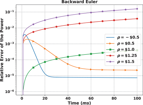
To motivate this point of view, a simple numerical study to show the limitation of the BE method was performed on a point kinetics equation (PKE) problem with delayed neutron data shown in Table I. The PKE problem was simulated with time steps of 0.1 ms for 0.1 s using the BE scheme. The reference solution was calculated analytically. The results are shown in Fig. 1. It can be seen that the relative error of the power at the end of the simulation is around 4%, when the initial reactivity is 1.25 $, and 16% when the reactivity is 1.5 $. Since the transport solution is eventually corrected by the PKE solutions in the TML method (or other improved quasistatic methods), it would be impossible for the pin power results to become more accurate than the amplitude correction from the PKE solution.

TABLE I Delayed Parameters of a PKE Problem*

Delay Group	Delayed Neutron Yields	Precursor Decay Constants	Prompt Neutron Generation
	$\beta$	$\lambda$ (s^−1)	Time $\mathrm{\Lambda }$ (s)
1	2.5840E-4	0.0128	2.57E-5
2	1.5200E-3	0.0318
3	1.3908E-3	0.119
4	3.0704E-3	0.3181
5	1.1020E-3	1.4027
6	2.5840E-4	3.9286

*All the PKE models analyzed in this paper use the parameters listed here unless stated otherwise. These parameters are from the Nuclear Energy Agency Committee on Reactor Physics (NECRP) benchmark.²¹

Fig. 1. Accuracy of the BE method in various problems. The PKE problem is simulated for 0.1 s with time steps of 0.1 ms. The relative errors of the power are calculated for each time step. It can be seen that if a reactivity of 1.5 $ is inserted into the system, the relative error at the end of the simulation can be as large as 16%. The reference solutions were generated analytically.

One motivation to introduce high-order methods is that high-order methods can potentially have higher accuracy and lower computational cost than low-order methods for a given time interval. A more important motivation is that in the foreseeable future, researchers in the neutronics community will apply high-order spatial discretization methods (mainly finite element methods) to the spatial kinetics problem (with a smoothly varying operator), and the neutronics problems and the feedback will be tightly coupled and solved together. In this case, high-order time-integration methods may be used. Otherwise, the error is highly likely to be determined by the temporal error rather than the spatial error.

The most popular high-order methods in the neutronics community are the $\theta$-method,^4–6 the backward differentiation formula⁷ (BDF), and the Runge-Kutta (RK) methods.⁸ A thorough review of these methods can be found in Ref. 9. The $\theta$-method can have at most second-order accuracy. When increasing the order of accuracy through the BDF or RK methods, the implementation becomes more complicated and the fundamental limits in the stability or efficiency of these methods also arise. For example, there exists no stable BDF method of order greater than six, and high-order implicit RK methods can be extremely computationally expensive.¹⁰

An alternative approach to constructing high-order methods is based on accelerating the convergence of low-order schemes.¹¹ A representative method of this kind, called the spectral deferred correction (SDC) method, was first proposed in Ref. 11. The method was developed from the classical deferred correction method.¹² Deferred correction methods can be arbitrary-order accurate theoretically, and extremely stable for stiff problems, even when the order of accuracy is very high. The deferred correction method consists of two parts, a prediction step and multiple correction steps to calculate the error. The most attractive feature of deferred correction methods is that the method is constructed based on a single low-order time-integration scheme [e.g., BE or forward Euler (FE)]. The difference between the SDC method and the classical deferred correction method is that spectral integration, discussed in Sec. II.B.2, is used. The method is straightforward to implement, and the order of accuracy can be adjusted readily without altering the implementation. This feature of the method also presents advantages to adaptive time-stepping schemes where an estimate of the truncation error of the step can be readily computed. In the field of nuclear engineering, some researchers have introduced SDC or other deferred correction methods to solve the PKE (Refs. 13 and 14). Researchers in related fields have introduced the SDC method and its variants to construct high-order stable solvers and have performed stable and efficient high-order simulations for radiation transport and multiphysics problems.^15–17

In this paper, we present the fundamental details of the SDC method and its application to solve PKEs, in general, and for the TML method in MPACT (Refs. 2 and 18). Compared to the research performed in Refs. 13 and 14, which is based on the Gauss Radau quadrature, the research performed here makes the following contributions. The implementation of the SDC method is based on the Gauss-Legendre quadrature. An effective way to obtain the integration matrix is derived and discussed in Sec. II.B.2. A new right endpoint evaluation approach is presented that can help the SDC method achieve 2M-th order accuracy when $M$ quadrature nodes are used. We also provide the derivation for implementing the SDC based on the low-order solver that is based on the commonly used analytical precursor integration approach. The application of the SDC method is then extended to the nonlinear PKE or PKE with linear energy feedback¹⁹ (PKE-EF), which is a simple low-order model for the neutronics problem coupled with feedback from thermal hydraulics (TH).

Though these problems are simple, the methodologies developed for solving the coupled precursor, feedback equations, and PKEs with SDC provide important insights, especially for practical considerations in the implementation. The stability of the SDC method is also shown. Numerical results support that SDC is effective in obtaining accurate results. This work is a necessary first step forward for investigations building on the methods developed here, particularly in the development of new, high-order, stable, and efficient solvers for transient neutron transport calculations.

The remainder of this paper is organized as follows. The description of the problems of interest and background about SDC are presented first in Sec. II. The various implementations of SDC for PKE and PKE-EF problems are shown in Sec. III. Numerical results, including the order of accuracy, stability, efficiency, and accuracy in the solution of EPKE for TML in MPACT, are shown in Sec. IV. A summary and areas of future work are provided in Sec. V. Finally, the work presented in this paper was extended from part of the PhD thesis of the first author.²⁰

II. THEORY AND METHODOLOGY

II.A. Problems of Interest

In this paper, we are interested in the point kinetics model and the nonlinear PKE-EF model.¹⁹ PKE-EF can be written as

(1) $\frac{dp(t)}{dt}=\frac{\rho (t)-\beta (t)}{\mathrm{\Lambda }(t)}p(t)+\frac{1}{{\mathrm{\Lambda }}_0}\sum _{k=1}^K{\lambda }_k(t){\xi }_k(t),$(1)

(2) $\begin{array}{rl}& \frac{d{\xi }_k(t)}{dt}=\frac{{\mathrm{\Lambda }}_0}{\mathrm{\Lambda }(t)}{\beta }_k(t)p(t)-{\lambda }_k(t){\xi }_k(t),k=1,2,\cdots K\end{array},$(2)

(3) $\rho (t)={\rho }^{ex}(t)+{\gamma }_{d}Q(t),$(3)

and

(4) $\frac{dQ(t)}{dt}=-{\lambda }_{H}Q(t)+p(t)-p(0),$(4)

where the notations are consistent with Ref. 19:

$p$	=	= power
$k$	=	= group index of the delayed neutron precursor with $K$ as the number of delayed neutron precursor groups
$\xi$	=	= neutron precursor density
$Q$	=	= total energy deposited
${\lambda }_H$	=	= heat release constant indicating the fraction of the total energy that is removed out of reactor per unit time
$\mathrm{\$}$	=	= unit of the reactivity (a reactivity in the amount of ${\sum }_{k=1}^K{\beta }_k$ is called 1 dollar)
$fp$	=	= full power
s	=	= second
${\rho }^{ex}$	=	= external reactivity.

A typical group of delayed parameters are shown in Table I. In Eq. (3)(3) $\rho (t)={\rho }^{ex}(t)+{\gamma }_{d}Q(t),$(3) , ${\gamma }_d$ is the feedback coefficient and

(5) ${\gamma }_d\approx -0.8\text{rdollar}/fp\cdot \mathrm{s}$(5)

is typical for “[fast breeder reactor] and [light water reactor] oxide-fueled power reactors.”¹⁹

The PKE model is a simplified form of the PKE-EF model with ${\gamma }_d=0$. Let the vector $\mathbf{P}(t)={\left[\begin{array}{c}p(t),{\xi }_1(t),\cdots {\xi }_K(t)\end{array}\right]}^T$ and define

(6) $\mathbf{E}(t)=\left(\begin{array}{cccccc}\frac{\rho (t)-\beta (t)}{\mathrm{\Lambda }(t)}& \frac{{\lambda }_1(t)}{{\mathrm{\Lambda }}_0}& \frac{{\lambda }_2(t)}{{\mathrm{\Lambda }}_0}& \cdots & \frac{{\lambda }_K(t)}{{\mathrm{\Lambda }}_0}& \hspace{0.17em}\\ \frac{{\mathrm{\Lambda }}_0}{\mathrm{\Lambda }(t)}{\beta }_1(t)& -{\lambda }_1(t)& \hspace{0.17em}& \hspace{0.17em}& \hspace{0.17em}& \hspace{0.17em}\\ \frac{{\mathrm{\Lambda }}_0}{\mathrm{\Lambda }(t)}{\beta }_2(t)& \hspace{0.17em}& -{\lambda }_2(t)& \hspace{0.17em}& \hspace{0.17em}& \hspace{0.17em}\\ ⋮& \hspace{0.17em}& \hspace{0.17em}& \ddots & \hspace{0.17em}& \hspace{0.17em}\\ \frac{{\mathrm{\Lambda }}_0}{\mathrm{\Lambda }(t)}{\beta }_K(t)& \hspace{0.17em}& \hspace{0.17em}& \cdots & -{\lambda }_K(t)& \hspace{0.17em}\end{array}\right).$(6)

The system of PKE now can be expressed in operator notation as

(7) $\frac{d\mathbf{P}(t)}{dt}=\mathbf{E}(t)\mathbf{P}(t).$(7)

II.B. Mathematical Preliminaries of SDC

In this section, we present the mathematical preliminaries for understanding the SDC method. Briefly, SDC is a method based on calculating the error of the solution from low-order time integrators, and then correcting the solution with the calculated errors. In Sec. II.B.1, we focus on how the error is defined and calculated.

II.B.1. Error Equation

The SDC method was developed based on the Picard integral equation. The governing equation of the IVP for the time interval $[a,b]$ is assumed to be of the following form:

(8) $\frac{d\mathrm{\Psi }}{dt}=F(t,\mathrm{\Psi }),t\in [a,b]$(8)

and

(9) $\mathrm{\Psi }(a)={\mathrm{\Psi }}_a,$(9)

where ${\mathrm{\Psi }}_a$ is the initial condition, and $\mathrm{\Psi }(t)$ is the solution we want to obtain; both exist in the $N$ dimension complex space ${\mathbb{C}}^N$. Also, $F:\mathbb{R}\times {\mathbb{C}}^N\to {\mathbb{C}}^N$. We also assume that $F\in C^{\mathrm{\infty }}(\mathbb{R}\times {\mathbb{C}}^N)$, i.e., $F$ is infinitely differentiable or sufficiently smooth. Given this, the solution $\mathrm{\Psi }$ may be written as

(10) $\mathrm{\Psi }(t)={\int }_a^{t}F(\tau ,\mathrm{\Psi }(\tau ))d\tau +{\mathrm{\Psi }}_a.$(10)

It should also be noted that the range $[a,b]$ is typically assumed to be a single time step.

Now, suppose that we have obtained the approximate solution $\tilde{\mathrm{\Psi }}(t)$ based on a simple time-integration technique like BE. Then we may write the error of the solution denoted by $\delta (t)$ as

(11) $\delta (t)=\mathrm{\Psi }(t)-\tilde{\mathrm{\Psi }}(t)={\int }_a^{t}F(\tau ,\mathrm{\Psi }(\tau ))d\tau +{\mathrm{\Psi }}_a-\tilde{\mathrm{\Psi }}(t).$(11)

This definition of the error can be substituted back into Eq. (11(11) $\delta (t)=\mathrm{\Psi }(t)-\tilde{\mathrm{\Psi }}(t)={\int }_a^{t}F(\tau ,\mathrm{\Psi }(\tau ))d\tau +{\mathrm{\Psi }}_a-\tilde{\mathrm{\Psi }}(t).$(11) ), leading to the following expression for the error given by Eq. (12)(12) $\delta (t)={\int }_a^{t}F(\tau ,\tilde{\mathrm{\Psi }}(\tau )+\delta (\tau ))d\tau +{\mathrm{\Psi }}_a-\tilde{\mathrm{\Psi }}(t).$(12) :

(12) $\delta (t)={\int }_a^{t}F(\tau ,\tilde{\mathrm{\Psi }}(\tau )+\delta (\tau ))d\tau +{\mathrm{\Psi }}_a-\tilde{\mathrm{\Psi }}(t).$(12)

Equation (12)(12) $\delta (t)={\int }_a^{t}F(\tau ,\tilde{\mathrm{\Psi }}(\tau )+\delta (\tau ))d\tau +{\mathrm{\Psi }}_a-\tilde{\mathrm{\Psi }}(t).$(12) is still quite complicated to evaluate, but it can be simplified by decoupling $\delta$ from $\tilde{\mathrm{\Psi }}$ with the following procedure. First, Eq. (12)(12) $\delta (t)={\int }_a^{t}F(\tau ,\tilde{\mathrm{\Psi }}(\tau )+\delta (\tau ))d\tau +{\mathrm{\Psi }}_a-\tilde{\mathrm{\Psi }}(t).$(12) for the error is rewritten as Eq. (13(13) $\delta (t)={\displaystyle {\int }_a^{t}F}(\tau ,\Psi (\tau )+\delta (\tau ))d\tau -{\displaystyle {\int }_a^{t}F}(\tau ,\Psi (\tau ))d\tau +ϵ(t),$(13) ),

(13) $\delta (t)={\displaystyle {\int }_a^{t}F}(\tau ,\Psi (\tau )+\delta (\tau ))d\tau -{\displaystyle {\int }_a^{t}F}(\tau ,\Psi (\tau ))d\tau +ϵ(t),$(13)

with

(14) $ϵ(t)={\displaystyle {\int }_a^{t}F}(\tau ,\Psi (\tau ))d\tau +{\Psi }_a-\Psi (t),$(14)

where $ϵ(t)$ is called the residual function.¹¹ The details of how it is evaluated are discussed next in Sec. II.B.2. Excluding the residual function, the remainder of the right side of Eq. (13)(13) $\delta (t)={\displaystyle {\int }_a^{t}F}(\tau ,\Psi (\tau )+\delta (\tau ))d\tau -{\displaystyle {\int }_a^{t}F}(\tau ,\Psi (\tau ))d\tau +ϵ(t),$(13) is composed of two integrals. By combining the integrals, we may define the function $G:\mathbb{R}\times {\mathbb{C}}^n\to {\mathbb{C}}^n$,

(15) $G(t,\delta )=F(t,\tilde{\mathrm{\Psi }}(t)+\delta (t))-F(t,\tilde{\mathrm{\Psi }}(t)),$(15)

as the argument of the integral. Substituting Eq. (15)(15) $G(t,\delta )=F(t,\tilde{\mathrm{\Psi }}(t)+\delta (t))-F(t,\tilde{\mathrm{\Psi }}(t)),$(15) into Eq. (13)(13) $\delta (t)={\displaystyle {\int }_a^{t}F}(\tau ,\Psi (\tau )+\delta (\tau ))d\tau -{\displaystyle {\int }_a^{t}F}(\tau ,\Psi (\tau ))d\tau +ϵ(t),$(13) yields

(16) $\delta (t)-{\int }_a^{t}G(\tau ,\delta (\tau ))d\tau =ϵ(t).$(16)

This is the governing equation for the error to correct in deferred correction methods. In differential form, Eq. (16)(16) $\delta (t)-{\int }_a^{t}G(\tau ,\delta (\tau ))d\tau =ϵ(t).$(16) is

(17) $\frac{d\delta (t)}{dt}=G(t,\delta (t))+\frac{dϵ(t)}{dt}.$(17)

For the linear problem with

(18) $F(t,{\mathrm{\Psi }}_1+{\mathrm{\Psi }}_2)=F(t,{\mathrm{\Psi }}_1)+F(t,{\mathrm{\Psi }}_2),$(18)

we have

(19) $G(t,\delta (t))=F(t,\delta (t)).$(19)

This results in equations for the error that have a form similar to Eq. (10)(10) $\mathrm{\Psi }(t)={\int }_a^{t}F(\tau ,\mathrm{\Psi }(\tau ))d\tau +{\mathrm{\Psi }}_a.$(10) or Eq. (8)(8) $\frac{d\mathrm{\Psi }}{dt}=F(t,\mathrm{\Psi }),t\in [a,b]$(8) . In recognizing this, the insight of deferred correction methods is that the error equations [Eqs. (16)(16) $\delta (t)-{\int }_a^{t}G(\tau ,\delta (\tau ))d\tau =ϵ(t).$(16) and (17(17) $\frac{d\delta (t)}{dt}=G(t,\delta (t))+\frac{dϵ(t)}{dt}.$(17) )] can also be solved using the same low-order method as the original IVP if we know the residual function $ϵ(t)$. Once $\delta$ is obtained, the corrected solution is readily calculated as

(20) $\mathrm{\Psi }(b)=\tilde{\mathrm{\Psi }}(b)+\delta (b).$(20)

Consequently, the goal of deferred correction methods is to calculate the residual function to obtain the correction for the error in Eq. (20)(20) $\mathrm{\Psi }(b)=\tilde{\mathrm{\Psi }}(b)+\delta (b).$(20) . In the next few sections, the details of how the residual function can be calculated and used to obtain the error correction are given.

II.B.2. Spectral Integration of the Residual Function

To calculate the residual function, Eq. (8)(8) $\frac{d\mathrm{\Psi }}{dt}=F(t,\mathrm{\Psi }),t\in [a,b]$(8) must be solved with multiple time steps. Therefore, a fine grid is introduced inside the time range $[a,b]$. For the remainder of this paper, the time points in $[a,b]$ are referred to as nodes following the convention used in Ref. 11. First, we define $M$ as the number of nodes used within the time interval $a=t_0<t_1<t_2<\cdots t<t_M<=t_{M+1}=b$. In the standard deferred correction method, the nodes are equally spaced. In the SDC method the nodes are positioned more advantageously via a spectral quadrature to avoid Runge’s phenomenon.

Next, assume that the approximated solution ${\tilde{\mathrm{\Psi }}}_m$ has been obtained at each fine grid point $m$ in time. $F(t_m,{\tilde{\mathrm{\Psi }}}_m)$ is calculated for $m=1,2,3\cdots M$ and is denoted as $F_m$ for brevity. The continuous derivative $F(t)$ can be obtained via high-order Lagrange interpolation. Then, the residual function can be obtained by integrating $F(t)$ analytically. To illustrate this, let the matrices

(21) $\mathbf{F}={\left[\begin{array}{c}{F}_1,\cdots ,F_m,\cdots ,F_M\end{array}\right]}^T\in {\mathbb{C}}^{M\times N}$(21)

and

(22) $\mathbf{I}={\left[\begin{array}{c}{\int }_a^{t_1}F(t)d\tau ,{\int }_a^{t_2}F(t)d\tau ,\cdots {\int }_a^{t_M}F(t)d\tau \end{array}\right]}^T\in {\mathbb{C}}^{M\times N}.$(22)

Here, $F_m$ is already a vector. It turns out that

(23) $\mathbf{I}=\mathbf{S}\mathbf{F}\in {\mathbb{C}}^{M\times N},$(23)

where $\mathbf{S}$ is the integration operator and $\mathbf{S}\in {\mathbb{C}}^{M\times M}$. The process of obtaining $\mathbf{I}$ from $\mathbf{F}$ is a linear mapping.¹¹ This is the general procedure of the deferred correction method. Since the Lagrange interpolation is affected by the size of the substeps or when $b-a$ changes, then $\mathbf{S}$ will change as a result.

Compared to the classical deferred correction method, the improvement from SDC is that time nodes for the SDC are obtained spectrally. Therefore, $\mathbf{S}$ can be efficiently evaluated via spectral integration.²²

The matrix $\mathbf{S}$ obtained via spectral integration in Eq. (23)(23) $\mathbf{I}=\mathbf{S}\mathbf{F}\in {\mathbb{C}}^{M\times N},$(23) is called the spectral integration matrix. The matrix can be very efficiently evaluated when the nodes are generated with the Gauss-Legendre quadrature set. For the remainder of this subsection, we provide one simple derivation to calculate the integration matrix.

To illustrate how this is calculated, suppose that we have obtained abscissas $\mathbf{x}$ and the weights $\mathbf{w}$ for the Gauss-Legendre quadrature set with $M$ points. The m-th internal node $t_m$ is determined by

(24) $t_m=\frac{b+a}{2}+\frac{b-a}{2}{x}_m=\frac{b+a}{2}+\frac{h}{2}{x}_m,$(24)

where $h$ is the step size, i.e., $b-a$, and $x_m$ is the m-th abscissa for the Gauss-Legendre quadrature. Next, let the vector $\mathbf{f}\in {\mathbb{C}}^M$ be a column vector of $F$. Then the Lagrange interpolation is written as

(25) $\hat{f}(t)=\sum _{l=0}^{M-1}{c}_l{\hat{P}}_l(t)=\sum _{l=0}^{M-1}{c}_l{P}_l(\frac{2t-(a+b)}{h}),$(25)

where $P_l$ is the Legendre polynomial of order $l$, and

(26) ${\hat{P}}_l(t)=P_l(\frac{2t-(a+b)}{h}).$(26)

The coefficients $c_l$ are

(27) $\begin{array}{cc}{c}_l& =\frac{2l+1}{2}{\int }_{-1}^1\hat{f}(\frac{h}{2}\tau +\frac{a+b}{2})P_l(\tau )d\tau \\ \hspace{0.17em}& =\frac{2l+1}{2}\sum _{m=1}^M{w}_m{f}_m{P}_l(x_m)=V_l^T\mathbf{f}.\end{array}$(27)

Here, the Gauss quadrature rule has been used and is accurate since the degree of the polynomial integrated is smaller than $2M-1$; $V_l$ is the column vector

(28) $V_l=\frac{2l+1}{2}[w_1{P}_l(x_1),w_2{P}_l(x_2),\cdots w_M{P}_l(x_M){]}^T\in {\mathbb{C}}^M,$(28)

and we define the matrix $\mathbf{V}$ as

(29) $\mathbf{V}=\left[\begin{array}{c}{V}_0,V_1,\cdots V_{M-1}\end{array}\right].$(29)

Substituting Eq. (27)(27) $\begin{array}{cc}{c}_l& =\frac{2l+1}{2}{\int }_{-1}^1\hat{f}(\frac{h}{2}\tau +\frac{a+b}{2})P_l(\tau )d\tau \\ \hspace{0.17em}& =\frac{2l+1}{2}\sum _{m=1}^M{w}_m{f}_m{P}_l(x_m)=V_l^T\mathbf{f}.\end{array}$(27) into Eq. (25(25) $\hat{f}(t)=\sum _{l=0}^{M-1}{c}_l{\hat{P}}_l(t)=\sum _{l=0}^{M-1}{c}_l{P}_l(\frac{2t-(a+b)}{h}),$(25) ), and letting the vector

(30) $\stackrel{\mathbf{ˆ}}{\mathbf{P}}(t)=\left[\begin{array}{c}{\hat{P}}_0(t),{\hat{P}}_1(t)\cdots {\hat{P}}_{M-1}(t)\end{array}\right]\in {\mathbb{C}}^{1\times M},$(30)

yields

(31) $\hat{f}(t)=\stackrel{\mathbf{ˆ}}{\mathbf{P}}(t){\mathbf{V}}^T\mathbf{f}.$(31)

Following this, we introduce the matrix $\bar{\mathbf{V}}\in {\mathbf{C}}^{M\times M}$ and its m-th row vector ${\bar{\mathbf{v}}}_m$. The component ${\bar{v}}_{l+1,m}$ is defined via the integral

(32) $\begin{array}{rl}& {\int }_a^{t_m}{\hat{P}}_l(\tau )d\tau =\frac{h}{2}{\int }_{-1}^{x_m}{P}_l(s)ds\\ & =\frac{x_m+1}{2}\frac{h}{2}{\int }_{-1}^1{P}_l((x_m+1)(s^{\mathrm{\prime }}+1)-1)d{s}^{\mathrm{\prime }}\\ & =\frac{x_m+1}{2}\frac{h}{2}\sum _{i=1}^M{P}_l((x_m+1)(x_i+1)-1)w_i\\ & =\frac{h}{2}{\bar{v}}_{l+1,m}.& (32)\end{array}$(32)

The integration term $i_m$ now becomes

(33) $i_m={\int }_a^{t_m}\hat{f}(\tau )d\tau =\frac{h}{2}{\bar{\mathbf{v}}}_m{\mathbf{V}}^T\mathbf{f}.$(33)

Next, we define the column vector

(34) $\mathbf{i}={\left[\begin{array}{c}{i}_1,i_2\cdots i_M\end{array}\right]}^T\in {\mathcal{C}}^{M\times 1},$(34)

which gives

(35) $\mathbf{i}=\frac{h}{2}\bar{\mathbf{V}}{\mathbf{V}}^T\mathbf{f}.$(35)

The $M\times M$ matrix ${\mathbf{S}}_b$ is denoted by

(36) ${\mathbf{S}}_b=\bar{\mathbf{V}}{\mathbf{V}}^T.$(36)

${\mathbf{S}}_b$ now only depends on $M$, thus it can be precomputed. From here, it should be straightforward to see that the integration matrix $\mathbf{S}$ is simply

(37) $\mathbf{S}=\frac{h}{2}{\mathbf{S}}_b.$(37)

Finally, Eq. (23)(23) $\mathbf{I}=\mathbf{S}\mathbf{F}\in {\mathbb{C}}^{M\times N},$(23) can be written as

(38) $\mathbf{I}=\frac{h}{2}{\mathbf{S}}_b\mathbf{F}.$(38)

Reference 10 provides a derivation for the spectral integration matrix that relies on matrix inversion (MI). However, this is relatively more complicated. Thus, the process presented here provides an alternative way to calculate the spectral integration matrix directly. As a result, this formulation has the advantage that $S$ can be readily obtained for cases with varying time steps and would not require multiple MIs.

Previously, we made use of the Gauss-Legendre quadrature to define the spectral nodes. However, other spectral quadrature sets exist, with some popular choices being the Chebyshev and Gauss-Lobatto quadrature sets.^10,17 The choice of quadrature set affects the derivation of the spectral integration matrix and slightly affects the stability region of the SDC. A detailed discussion on the use of various quadrature sets can be found in Ref. 10. For now, we proceed using the Gauss-Legendre quadrature sets because they are commonly used in the nuclear reactor physics field.

The (M-1)-th order approximation of the residual function given by Eq. (14)(14) $ϵ(t)={\displaystyle {\int }_a^{t}F}(\tau ,\Psi (\tau ))d\tau +{\Psi }_a-\Psi (t),$(14) at the spectral time nodes can be written as

(39) $\sigma (\bar{\mathrm{\Psi }})={\mathbf{F}}^{\mathbf{T}}{\mathbf{S}}^{\mathbf{T}}+{\bar{\mathrm{\Psi }}}_a-\bar{\mathrm{\Psi }},$(39)

with

$\bar{\mathrm{\Psi }}=\left[\begin{array}{c}\tilde{\mathrm{\Psi }}(t_1),\tilde{\mathrm{\Psi }}(t_2),\cdots ,\tilde{\mathrm{\Psi }}(t_M)\end{array}\right],$

${\bar{\mathrm{\Psi }}}_a=\left[\begin{array}{c}\tilde{\mathrm{\Psi }}(a),\tilde{\mathrm{\Psi }}(a),\cdots ,\tilde{\mathrm{\Psi }}(a)\end{array}\right]$

and

(40) $\sigma ,\bar{\mathrm{\Psi }},{\bar{\mathrm{\Psi }}}_a\in {\mathbb{C}}^{N\times M}.$(40)

Here, the notation $\sigma$ is the same as that in Ref. 11 to indicate that $\sigma$ is a higher-order approximation to the residual $ϵ.$

II.B.3. Error Correction

The error $\delta (t)$ needed to correct the approximate solution $\tilde{\mathrm{\Psi }}(t)$ is obtained by solving Eq. (16)(16) $\delta (t)-{\int }_a^{t}G(\tau ,\delta (\tau ))d\tau =ϵ(t).$(16) with a low-order method. It is recommended that the FE method (for nonstiff problems) or BE method (for stiff problems) be used.¹¹ The solution of Eq. (16)(16) $\delta (t)-{\int }_a^{t}G(\tau ,\delta (\tau ))d\tau =ϵ(t).$(16) with the FE method for nonstiff problems is given by the formula

(41) ${\delta }_{m+1}={\delta }_m+G(t_m,{\delta }_m)h_{m+1}+{\sigma }_{m+1}-{\sigma }_m,$(41)

and the BE method for stiff problems is

(42) ${\delta }_{m+1}={\delta }_m+G(t_{m+1},{\delta }_{m+1})h_{m+1}+{\sigma }_{m+1}-{\sigma }_m$(42)

for $m=1,2,\cdots M$ and $h_{m+1}=t_{m+1}-t_m$. $G$ has been defined in Eq. (15)(15) $G(t,\delta )=F(t,\tilde{\mathrm{\Psi }}(t)+\delta (t))-F(t,\tilde{\mathrm{\Psi }}(t)),$(15) . Furthermore, sometimes, $G$ can be partitioned as

(43) $G=G_I+G_E,$(43)

where $G_I$ is stiff and can be solved implicitly, and $G_E$ is nonstiff and can be solved explicitly. Then it is also possible to solve Eq. (16)(16) $\delta (t)-{\int }_a^{t}G(\tau ,\delta (\tau ))d\tau =ϵ(t).$(16) in the implicit-explicit (IMEX) way,¹⁵

(44) $\begin{array}{rl}& {\delta }_{m+1}={\delta }_m+G_I(t_{m+1},{\delta }_{m+1})h_{m+1}\\ & +G_E(t_m,{\delta }_m)h_{m+1}+{\sigma }_{m+1}-{\sigma }_m.\end{array}$(44)

II.B.4. SDC Algorithm

Now the overall procedure of the SDC is given. The algorithm for the SDC method is presented in Algorithm 1.

Table

Algorithm 1 General Procedure for SDC.

1: Input the number of corrections $\mathit{J}$ and initial condition for time $a$, i.e., ${\mathrm{\Psi }}_a$.

2: Prediction: Compute the initial estimate of ${\bar{\mathbf{\Psi }}}^{(0)}$ at the time nodes $t_1\cdots t_M$ and at b if needed with the low-order solver.

Correction:

3: for $j=1,2,\dots ,J$ do

4:     Compute the residual function ${\sigma }^{\left(j\right)}$ at each node via spectral integration.

5:     Compute the error ${\delta }^{\left(j\right)}$ via the low-order solvers.

6:     Update the solution for the j^th correction by ${\bar{\Psi }}^{(j)}\left(t_m\right)={\bar{\Psi }}^{(j-1)}\left(t_m\right)+{\delta }^{(j)}\left(t_m\right)$.

7: end for

8: Evaluation at b if needed.

The SDC for the solution of Eq. (8)(8) $\frac{d\mathrm{\Psi }}{dt}=F(t,\mathrm{\Psi }),t\in [a,b]$(8) is a prediction-correction process. During the prediction step, the solution is computed with a low-order numerical method at the spectral time nodes $t_0,t_1,\dots ,t_{M+1}$. This solution is denoted as ${\overline{\Psi }}^{\left(0\right)}$. During the correction step, there are $J$ correction “sweeps.” For the j-th correction, the residual ${\sigma }^{(j)}$ is calculated with ${\bar{\mathrm{\Psi }}}^{\left(j-1\right)}$ using Eq. (39)(39) $\sigma (\bar{\mathrm{\Psi }})={\mathbf{F}}^{\mathbf{T}}{\mathbf{S}}^{\mathbf{T}}+{\bar{\mathrm{\Psi }}}_a-\bar{\mathrm{\Psi }},$(39) . The error is then calculated with one of Eqs. (41)(41) ${\delta }_{m+1}={\delta }_m+G(t_m,{\delta }_m)h_{m+1}+{\sigma }_{m+1}-{\sigma }_m,$(41) , (42(42) ${\delta }_{m+1}={\delta }_m+G(t_{m+1},{\delta }_{m+1})h_{m+1}+{\sigma }_{m+1}-{\sigma }_m$(42) ), or (44(44) $\begin{array}{rl}& {\delta }_{m+1}={\delta }_m+G_I(t_{m+1},{\delta }_{m+1})h_{m+1}\\ & +G_E(t_m,{\delta }_m)h_{m+1}+{\sigma }_{m+1}-{\sigma }_m.\end{array}$(44) ), and is used to correct the solution ${\bar{\mathrm{\Psi }}}^{\left(j-1\right)}$ via Eq. (20)(20) $\mathrm{\Psi }(b)=\tilde{\mathrm{\Psi }}(b)+\delta (b).$(20) . The updated solution is then ${\bar{\mathrm{\Psi }}}^{\left(j\right)}$.

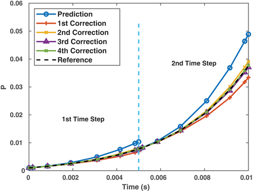
Additionally, Fig. 2 provides an illustration of the method. For each time step, the predicted solution has a relatively large error. Then multiple corrections are performed. The solution becomes more accurate with each correction performed. Eventually, after the last correction, the solution becomes very accurate.

Fig. 2. Illustration of the SDC scheme.

II.C. Right Endpoint Evaluation

It should also be noted that the error is not obtained directly for the time point $b$ as might be indicated by Algorithm 1. The reason is that $t_M$ should be smaller than $b$. There are multiple ways to calculate the error or the solution at $b$, and some are more advantageous than others. This is an important practical detail to implementing the SDC method. The right endpoint treatment also influences the stability region of the overall method. This aspect is investigated in more detail in Sec. IV.B. For now, we wish to briefly introduce some of the possible approaches to right endpoint evaluation:

1. Extrapolation (EP): The solution at $b$ is not calculated for both the prediction and correction. After $J$ corrections, the solution $\mathrm{\Psi }(b)$ is then obtained by extrapolating the Lagrange polynomials.^10,11 Instead of extrapolating with the Lagrange polynomials, it is also possible to use the spectral integration

(45) $\mathrm{\Psi }(b)={\bar{\psi }}^{\left(J\right)}\mathbf{V}\mathbf{1},$(45)

where $\mathbf{1}\in {\mathbb{C}}^M$ is a column vector with all the components equal to 1.

• 2. Right-hand approach¹⁰: If the time step size is $h=\frac{2}{1+x_M}(a-b)$, then $t_M=b$ and $\mathrm{\Psi }(b)={\mathrm{\Psi }}^{\left(J\right)}(t_m)$. This approach is not investigated here.

• 3. Gaussian integration (GI): The residual at $b$ is calculated via numerical integration using a Gauss quadrature

(46) ${\sigma }_{M+1}=\frac{h}{2}{\mathbf{F}}^T\mathbf{w},$(46)

where $\mathbf{w}$ is the column vector of the weights. Therefore, we have $M+1$ low-order solves per prediction and correction steps. Then the error at $b$ is solved with the residual.

When the problem is not that stiff, then it is possible to use the following:

(47) $\mathrm{\Psi }(b)=\mathrm{\Psi }(a)+{\sigma }_{M+1}.$(47)

However, this method is not stable for stiff problems, and we consider this method to better understand that limitation. Additionally, we consider the GI method because, so far, we have not found any other references that report this treatment. Although, since the GI method is straightforward to implement, we acknowledge it is possible that other researchers have investigated or adopted this method.

It should be noted that it is possible to have $t_M=b$ when other quadrature sets are used. For example, the right endpoint is included in the Gauss-Lobatto quadrature and the right-hand Gauss-Radau quadrature. Then there is no need for caring about the right endpoint treatment since we can have $\mathrm{\Psi }(b)={\mathrm{\Psi }}^{\left(J\right)}(t_m)$. But the maximum order of convergence allowed will be reduced, and the stability can be altered.¹¹

II.D. Other Remarks About SDC

Finally, it is worth acknowledging that there are a few other techniques that have been developed that we do not consider further here. In Ref. 15, the correction and solution processes are combined together to improve the stability and the convergence rate. Additionally, a trapezoidal method has also been investigated for the prediction and correction steps.²³ However, the improvement in this case was small because the time nodes were not equi-spaced, and the resulting SDC method was not $L$-stable. Multigrid methods and parareal algorithms can be applied together with SDC to further improve the accuracy and efficiency.^24,25

III. SDC FOR PKE AND PKE-EF

The procedures described in Sec. II.B.3 provide a skeleton for the implementation of the SDC method. The actual implementation of the SDC method depends on the choice of the low-order time-integration scheme and right-end evaluation technique. Here we provide implementation details of the SDC solver for the PKE-EF using three different low-order integrators.

III.A. Low-Order Time Integration

In this section, we introduce three different implementations of the low-order solvers for the solution of the prediction step and error of the correction sweeps in PKE.

The PKE is written in operator notation [Eq. (7)(7) $\frac{d\mathbf{P}(t)}{dt}=\mathbf{E}(t)\mathbf{P}(t).$(7) revisited]:

$\frac{d\mathbf{P}(t)}{dt}=\mathbf{E}(t)\mathbf{P}(t).$

The first low-order method is referred to as MI. Suppose that the PKE is solved implicitly. During the prediction step,

(48) ${\mathbf{P}}_{m+1}=(I-\mathbf{E}{h}_{m+1}{)}^{-1}{\mathbf{P}}_m.$(48)

For the correction, since the operator $\mathbf{E}$ in Eq. (7)(7) $\frac{d\mathbf{P}(t)}{dt}=\mathbf{E}(t)\mathbf{P}(t).$(7) is linear, $G(t_m,{\delta }_m)$ may be written as

(49) $G(t_m,{\delta }_m)=\mathbf{E}(t_m){\delta }_m.$(49)

The BE solution of Eq. (42)(42) ${\delta }_{m+1}={\delta }_m+G(t_{m+1},{\delta }_{m+1})h_{m+1}+{\sigma }_{m+1}-{\sigma }_m$(42) is

(50) ${\delta }_{m+1}=(\mathbf{I}-\mathbf{E}{h}_{m+1}{)}^{-1}({\delta }_m+{\sigma }_{m+1}-{\sigma }_m).$(50)

This is a direct solution process involving a MI.

The second method is based on the IMEX partitioning approach described in Ref. 15. Here we refer to this method as operator splitting (OS) since the power is calculated first with the lagged precursor density, then the precursor density is calculated with the power. In this variation, the prediction step is

(51a) $p^{\left(m+1\right)}=\frac{p^{\left(m\right)}+\frac{1}{{\mathrm{\Lambda }}_0}{h}^{\left(m+1\right)}{\sum }_{k=1}^K{\lambda }_k^{\left(m+1\right)}{\xi }_k^{\left(m\right)}}{1-\frac{{\rho }^{\left(m+1\right)}-{\beta }^{\left(m+1\right)}}{{\mathrm{\Lambda }}^{\left(m+1\right)}}{h}^{\left(m+1\right)}}$(51a)

and

(51b) ${\xi }_k^{\left(m+1\right)}=\frac{{\xi }_k^{\left(m\right)}+h^{\left(m+1\right)}{\beta }_k^{\left(m+1\right)}\frac{{\Lambda }_0}{{\Lambda }^{\left(m+1\right)}}{p}^{\left(m+1\right)}}{1+{\lambda }_k^{\left(m+1\right)}{h}^{\left(m+1\right)}}1pt,k=1,\cdots K1pt.$(51b)

For the correction sweeps, the following expressions are used:

(52a) ${\delta }^{\left(m+1\right)}(p)=\frac{{\delta }^{\left(m\right)}(p)+\frac{1}{{\mathrm{\Lambda }}_0}{h}^{\left(m+1\right)}{\sum }_{k=1}^K{\lambda }_k^{\left(m+1\right)}{\delta }^{\left(m\right)}({\xi }_k)+{\sigma }_p^{\left(m+1\right)}-{\sigma }_p^{\left(m\right)}\hspace{0.17em}}{1-\frac{{\rho }^{\left(m+1\right)}-{\beta }^{\left(m+1\right)}}{{\mathrm{\Lambda }}^{\left(m+1\right)}}{h}^{\left(m+1\right)}}$(52a)

and

(52b) ${\delta }^{\left(m+1\right)}({\xi }_k)=\frac{{\delta }^{\left(m\right)}({\xi }_k)+h^{\left(m+1\right)}{\beta }_k^{\left(m+1\right)}\frac{{\mathrm{\Lambda }}_0}{{\mathrm{\Lambda }}^{\left(m+1\right)}}{\delta }^{\left(m+1\right)}(p)+{\sigma }_k^{\left(m+1\right)}-{\sigma }_k^{\left(m\right)}\hspace{0.17em}}{1+{\lambda }_k^{\left(m+1\right)}{h}^{\left(m+1\right)}},k=1,\cdots ,K.\hspace{0.17em}$(52b)

The MI is avoided through separating the operator applied on $p$ and $\xi$. The OS approach can also be understood as

(53) $\begin{array}{r}{\mathbf{P}}^{\left(m+1\right)}={\mathbf{P}}^{\left(m\right)}+\left({\mathbf{E}}_I^{\left(m+1\right)}{\mathbf{P}}^{\left(m+1\right)}+{\mathbf{E}}_E^{\left(m\right)}{\mathbf{P}}^{\left(m\right)}\right)h^{(m+1)}\end{array},$(53)

where

(54) ${\mathbf{E}}_I(t)=\left(\begin{array}{cccccc}\frac{\rho (t)-\beta (t)}{\mathrm{\Lambda }(t)}& \hspace{0.17em}& \hspace{0.17em}& \hspace{0.17em}& \hspace{0.17em}& \hspace{0.17em}\\ \frac{{\mathrm{\Lambda }}_0}{\mathrm{\Lambda }(t)}{\beta }_1& -{\lambda }_1(t)& \hspace{0.17em}& \hspace{0.17em}& \hspace{0.17em}& \hspace{0.17em}\\ \frac{{\mathrm{\Lambda }}_0}{\mathrm{\Lambda }(t)}{\beta }_2& \hspace{0.17em}& -{\lambda }_2(t)& \hspace{0.17em}& \hspace{0.17em}& \hspace{0.17em}\\ ⋮& \hspace{0.17em}& \hspace{0.17em}& \ddots & \hspace{0.17em}& \hspace{0.17em}\\ \frac{{\mathrm{\Lambda }}_0}{\mathrm{\Lambda }(t)}{\beta }_K(t)& \hspace{0.17em}& \hspace{0.17em}& \cdots & -{\lambda }_K(t)& \hspace{0.17em}\end{array}\right)$(54)

and

(55) ${\mathbf{E}}_E(t)=\left(\begin{array}{cc}0& \frac{1}{{\mathrm{\Lambda }}_0}\lambda (t)\\ \mathbf{0}& \mathbf{0}\end{array}\right),$(55)

with $\lambda =\left[\begin{array}{c}{\lambda }_1(t),{\lambda }_2(t),\cdots ,{\lambda }_K(t)\end{array}\right]$. In this method ${\mathbf{E}}_{\mathbf{I}}\mathbf{P}$ is treated implicitly and ${\mathbf{E}}_{\mathbf{E}}\mathbf{P}$ is treated explicitly. Therefore, this treatment can also be described as an IMEX procedure.

The third method is denoted FP because it uses first-order precursor integration to avoid the MI. First- or second-order precursor (SP) integration techniques are commonly used, including in MPACT (Ref. 2) and PARCS (Ref. 4). To obtain the FP solution, Eq. (2)(2) $\begin{array}{rl}& \frac{d{\xi }_k(t)}{dt}=\frac{{\mathrm{\Lambda }}_0}{\mathrm{\Lambda }(t)}{\beta }_k(t)p(t)-{\lambda }_k(t){\xi }_k(t),k=1,2,\cdots K\end{array},$(2) is first rewritten as

(56) $\begin{array}{r}\frac{d{\xi }_k(t)e^{{\lambda }_k^{\left(m+1\right)}(t-t^{\left(m\right)})}}{dt}=[{\lambda }_k^{\left(m+1\right)}{\xi }_k(t)+\frac{d{\xi }_k(t)}{dt}]e^{{\lambda }_k^{\left(m+1\right)}(t-t^{\left(m\right)})}=\frac{{\mathrm{\Lambda }}_0}{\mathrm{\Lambda }(t)}{\beta }_k(t)p(t)e^{{\lambda }_k^{\left(m+1\right)}(t-t^{\left(m\right)}),}\end{array}$(56)

where $\left(m+1\right)$ is the superscript rather than the subscript used to index the time point since the subscript $k$ is used to index the delayed neutron precursor. The derivation of the SP integration method can be found in Ref. 26.

To be able to integrate Eq. (56)(56) $\begin{array}{r}\frac{d{\xi }_k(t)e^{{\lambda }_k^{\left(m+1\right)}(t-t^{\left(m\right)})}}{dt}=[{\lambda }_k^{\left(m+1\right)}{\xi }_k(t)+\frac{d{\xi }_k(t)}{dt}]e^{{\lambda }_k^{\left(m+1\right)}(t-t^{\left(m\right)})}=\frac{{\mathrm{\Lambda }}_0}{\mathrm{\Lambda }(t)}{\beta }_k(t)p(t)e^{{\lambda }_k^{\left(m+1\right)}(t-t^{\left(m\right)}),}\end{array}$(56) analytically, $\frac{\beta (t)p(t)}{\mathrm{\Lambda }(t)}$ in the interval $[t_m,t_{m+1}]$ is approximated by the linear function

(57) $\begin{array}{rl}& \frac{{\beta }_k(t)p(t)}{\mathrm{\Lambda }(t)}=\frac{{\beta }_k^{\left(m\right)}{p}^{\left(m\right)}}{{\mathrm{\Lambda }}^{\left(m\right)}}(1-\gamma )+\frac{{\beta }_k^{\left(m+1\right)}{p}^{\left(m+1\right)}}{{\mathrm{\Lambda }}^{\left(m+1\right)}}\gamma ,\\ & \gamma =\frac{t-t^{\left(m\right)}}{t^{\left(m+1\right)}-t^{\left(m\right)}}.\end{array}$(57)

Substituting Eq. (57)(57) $\begin{array}{rl}& \frac{{\beta }_k(t)p(t)}{\mathrm{\Lambda }(t)}=\frac{{\beta }_k^{\left(m\right)}{p}^{\left(m\right)}}{{\mathrm{\Lambda }}^{\left(m\right)}}(1-\gamma )+\frac{{\beta }_k^{\left(m+1\right)}{p}^{\left(m+1\right)}}{{\mathrm{\Lambda }}^{\left(m+1\right)}}\gamma ,\\ & \gamma =\frac{t-t^{\left(m\right)}}{t^{\left(m+1\right)}-t^{\left(m\right)}}.\end{array}$(57) into Eq. (56)(56) $\begin{array}{r}\frac{d{\xi }_k(t)e^{{\lambda }_k^{\left(m+1\right)}(t-t^{\left(m\right)})}}{dt}=[{\lambda }_k^{\left(m+1\right)}{\xi }_k(t)+\frac{d{\xi }_k(t)}{dt}]e^{{\lambda }_k^{\left(m+1\right)}(t-t^{\left(m\right)})}=\frac{{\mathrm{\Lambda }}_0}{\mathrm{\Lambda }(t)}{\beta }_k(t)p(t)e^{{\lambda }_k^{\left(m+1\right)}(t-t^{\left(m\right)}),}\end{array}$(56) allows Eq. (56)(56) $\begin{array}{r}\frac{d{\xi }_k(t)e^{{\lambda }_k^{\left(m+1\right)}(t-t^{\left(m\right)})}}{dt}=[{\lambda }_k^{\left(m+1\right)}{\xi }_k(t)+\frac{d{\xi }_k(t)}{dt}]e^{{\lambda }_k^{\left(m+1\right)}(t-t^{\left(m\right)})}=\frac{{\mathrm{\Lambda }}_0}{\mathrm{\Lambda }(t)}{\beta }_k(t)p(t)e^{{\lambda }_k^{\left(m+1\right)}(t-t^{\left(m\right)}),}\end{array}$(56) to be integrated over $[t^{\left(m\right)},t^{\left(m+1\right)}]$ by using integrating factors. This yields

(58) $\begin{array}{rl}& {\xi }_k^{\left(m+1\right)}-{\xi }_k^{\left(m\right)}{e}^{-{\lambda }_k^{\left(m+1\right)}{h}_{m+1}}={\mathrm{\Lambda }}_0[\frac{{\beta }_k^{\left(m\right)}{p}^{\left(m\right)}}{{\mathrm{\Lambda }}^{\left(m\right)}}\frac{{\kappa }_0({\tilde{\lambda }}_k^{\left(m+1\right)})}{{\lambda }_k^{\left(m+1\right)}}\\ & +\left(\frac{{\beta }_k^{(m+1)}{p}^{(m+1)}}{{\mathrm{\Lambda }}^{(m+1)}}-\frac{{\beta }_k^{(m)}{p}^{(m)}}{{\mathrm{\Lambda }}^{(m)}}\right)\\ & \frac{{\kappa }_1({\tilde{\lambda }}_k^{\left(m+1\right)})}{{\lambda }_k^{\left(m+1\right)}}],\end{array}$(58)

where ${\kappa }_0(x)=1-exp(-x)$, ${\kappa }_1(x)=\frac{1-{\kappa }_0(x)}{x}$, and ${\tilde{\lambda }}_k^{\left(m+1\right)}={\lambda }_k^{\left(m+1\right)}{h}^{(m+1)}$. This now lets us write a closed form expression for the total delayed neutron source as

$\frac{1}{{\Lambda }_0}{\displaystyle \sum _{k=1}^K{\lambda }_k^{\left(m+1\right)}}{\xi }_k^{\left(m+1\right)}={\displaystyle \sum _{k=1}^K{\lambda }_k^{\left(m+1\right)}}{\xi }_k^{\left(m\right)}e-\lambda k(m+1{\Lambda }_0+\frac{{\displaystyle \sum _{k=1}^K{\beta }_k^{\left(m\right)}}[{\kappa }_0({\lambda }_k^{\left(m+1\right)})-{\kappa }_1({\lambda }_k^{\left(m+1\right)})]}{{\Lambda }^{\left(m\right)}}{p}^{\left(m\right)}+\frac{{\displaystyle \sum _{k=1}^K{\beta }_k^{\left(m+1\right)}}{\kappa }_1({\lambda }_k^{\left(m+1\right)})}{{\Lambda }^{\left(m+1\right)}}{p}^{\left(m+1\right)}.(59)$

Substituting Eq. (59)$\frac{1}{{\Lambda }_0}{\displaystyle \sum _{k=1}^K{\lambda }_k^{\left(m+1\right)}}{\xi }_k^{\left(m+1\right)}={\displaystyle \sum _{k=1}^K{\lambda }_k^{\left(m+1\right)}}{\xi }_k^{\left(m\right)}e-\lambda k(m+1{\Lambda }_0+\frac{{\displaystyle \sum _{k=1}^K{\beta }_k^{\left(m\right)}}[{\kappa }_0({\lambda }_k^{\left(m+1\right)})-{\kappa }_1({\lambda }_k^{\left(m+1\right)})]}{{\Lambda }^{\left(m\right)}}{p}^{\left(m\right)}+\frac{{\displaystyle \sum _{k=1}^K{\beta }_k^{\left(m+1\right)}}{\kappa }_1({\lambda }_k^{\left(m+1\right)})}{{\Lambda }^{\left(m+1\right)}}{p}^{\left(m+1\right)}.(59)$ into Eq. (6(6) $\mathbf{E}(t)=\left(\begin{array}{cccccc}\frac{\rho (t)-\beta (t)}{\mathrm{\Lambda }(t)}& \frac{{\lambda }_1(t)}{{\mathrm{\Lambda }}_0}& \frac{{\lambda }_2(t)}{{\mathrm{\Lambda }}_0}& \cdots & \frac{{\lambda }_K(t)}{{\mathrm{\Lambda }}_0}& \hspace{0.17em}\\ \frac{{\mathrm{\Lambda }}_0}{\mathrm{\Lambda }(t)}{\beta }_1(t)& -{\lambda }_1(t)& \hspace{0.17em}& \hspace{0.17em}& \hspace{0.17em}& \hspace{0.17em}\\ \frac{{\mathrm{\Lambda }}_0}{\mathrm{\Lambda }(t)}{\beta }_2(t)& \hspace{0.17em}& -{\lambda }_2(t)& \hspace{0.17em}& \hspace{0.17em}& \hspace{0.17em}\\ ⋮& \hspace{0.17em}& \hspace{0.17em}& \ddots & \hspace{0.17em}& \hspace{0.17em}\\ \frac{{\mathrm{\Lambda }}_0}{\mathrm{\Lambda }(t)}{\beta }_K(t)& \hspace{0.17em}& \hspace{0.17em}& \cdots & -{\lambda }_K(t)& \hspace{0.17em}\end{array}\right).$(6) ), and applying the BE method, gives

(60) $\frac{p^{\left(m+1\right)}-p^{\left(m\right)}}{h_{m+1}}=\frac{{\rho }^{\left(m+1\right)}-{\beta }^{\left(m+1\right)}}{{\mathrm{\Lambda }}^{\left(m+1\right)}}{p}^{\left(m+1\right)}+\frac{1}{{\mathrm{\Lambda }}_0}\sum _{k=1}^K{\lambda }_k^{\left(m+1\right)}{\xi }_k^{\left(m+1\right)}.$(60)

Next, we define the following expressions to simplify the final form:

(61a) ${\mathrm{\Omega }}_k^{\left(m+1\right)}=\frac{{\beta }_k^{\left(m+1\right)}}{{\lambda }_k^{\left(m+1\right)}}\frac{{\mathrm{\Lambda }}_0}{{\mathrm{\Lambda }}^{\left(m+1\right)}}{\kappa }_1({\tilde{\lambda }}_k^{\left(m+1\right)}),$(61a)

(61b) $S^{\left(m+1\right)}=\sum k=1K{\lambda }_k^{\left(m+1\right)}{\xi }_k^{\left(m\right)}e-\lambda k(m+1{\Lambda }_0+\sum k=1K{\beta }_k^{\left(m\right)}[{\kappa }_0({\lambda }_k^{\left(m+1\right)})-{\kappa }_1(\lambda k(m+1)]{\Lambda }^{\left(m\right)}{p}^{\left(m\right)}1pt,$(61b)

and

(61c) ${\tau }^{\left(m+1\right)}=\frac{{\sum }_{k=1}^K{\lambda }_k^{\left(m+1\right)}{\mathrm{\Omega }}_k^{\left(m+1\right)}}{{\mathrm{\Lambda }}_0}.$(61c)

Finally, substituting Eq. (59)$\frac{1}{{\Lambda }_0}{\displaystyle \sum _{k=1}^K{\lambda }_k^{\left(m+1\right)}}{\xi }_k^{\left(m+1\right)}={\displaystyle \sum _{k=1}^K{\lambda }_k^{\left(m+1\right)}}{\xi }_k^{\left(m\right)}e-\lambda k(m+1{\Lambda }_0+\frac{{\displaystyle \sum _{k=1}^K{\beta }_k^{\left(m\right)}}[{\kappa }_0({\lambda }_k^{\left(m+1\right)})-{\kappa }_1({\lambda }_k^{\left(m+1\right)})]}{{\Lambda }^{\left(m\right)}}{p}^{\left(m\right)}+\frac{{\displaystyle \sum _{k=1}^K{\beta }_k^{\left(m+1\right)}}{\kappa }_1({\lambda }_k^{\left(m+1\right)})}{{\Lambda }^{\left(m+1\right)}}{p}^{\left(m+1\right)}.(59)$ into Eq. (60)(60) $\frac{p^{\left(m+1\right)}-p^{\left(m\right)}}{h_{m+1}}=\frac{{\rho }^{\left(m+1\right)}-{\beta }^{\left(m+1\right)}}{{\mathrm{\Lambda }}^{\left(m+1\right)}}{p}^{\left(m+1\right)}+\frac{1}{{\mathrm{\Lambda }}_0}\sum _{k=1}^K{\lambda }_k^{\left(m+1\right)}{\xi }_k^{\left(m+1\right)}.$(60) and making use of Eq. (61)$\frac{1}{{\Lambda }_0}{\displaystyle \sum _{k=1}^K{\lambda }_k^{\left(m+1\right)}}{\xi }_k^{\left(m+1\right)}={\displaystyle \sum _{k=1}^K{\lambda }_k^{\left(m+1\right)}}{\xi }_k^{\left(m\right)}e-\lambda k(m+1{\Lambda }_0+\frac{{\displaystyle \sum _{k=1}^K{\beta }_k^{\left(m\right)}}[{\kappa }_0({\lambda }_k^{\left(m+1\right)})-{\kappa }_1({\lambda }_k^{\left(m+1\right)})]}{{\Lambda }^{\left(m\right)}}{p}^{\left(m\right)}+\frac{{\displaystyle \sum _{k=1}^K{\beta }_k^{\left(m+1\right)}}{\kappa }_1({\lambda }_k^{\left(m+1\right)})}{{\Lambda }^{\left(m+1\right)}}{p}^{\left(m+1\right)}.(59)$, yields the equations for the prediction step of the FP method,

(62a) $p^{\left(m+1\right)}=\frac{p^{\left(m\right)}+S^{\left(m+1\right)}{h}^{\left(m+1\right)}}{1-\tau h^{\left(m+1\right)}-\frac{{\rho }^{\left(m+1\right)}-{\beta }^{\left(m+1\right)}}{{\mathrm{\Lambda }}^{\left(m+1\right)}}{h}^{\left(m+1\right)}}$(62a)

and

(62b) $\begin{array}{rl}{\xi }_k^{\left(m+1\right)}={\xi }_k^{\left(m\right)}{e}^{-{\lambda }_k^{\left(m+1\right)}{h}^{\left(m+1\right)}}+{\mathrm{\Omega }}_k^{\left(m+1\right)}{p}^{\left(m+1\right)}+\frac{{\beta }_k^{\left(m\right)}{p}^{\left(m\right)}{\mathrm{\Lambda }}_0}{{\lambda }_k^{\left(m+1\right)}{\mathrm{\Lambda }}^{\left(m\right)}}& \\ [{\kappa }_0({\tilde{\lambda }}_k^{\left(m+1\right)})-{\kappa }_1({\tilde{\lambda }}_k^{\left(m+1\right)})].\end{array}$(62b)

For the correction step, the FP method slightly complicates the process for integrating the error with the same low-order method. The differential form of Eq. (16)(16) $\delta (t)-{\int }_a^{t}G(\tau ,\delta (\tau ))d\tau =ϵ(t).$(16) is

(63) $\frac{d\delta (t)}{dt}=\mathbf{E}\delta (t)+\frac{dϵ(t)}{dt}.$(63)

The error of the delayed neutron precursors $\delta ({\xi }_k)$ can be approximated with

(64) $\frac{d}{dt}\left(\delta ({\xi }_k)e^{{\lambda }_{k}t}\right)=e^{{\lambda }_{k}t}\frac{d\delta ({\xi }_k)}{dt}+{\lambda }_k{e}^{{\lambda }_{k}t}\delta ({\xi }_k)=\frac{{\mathrm{\Lambda }}_0}{\mathrm{\Lambda }(t)}{\beta }_k(t)\delta (p)e^{{\lambda }_{k}t}+\frac{d{ϵ}_k(t)}{dt}{e}^{{\lambda }_{k}t},$(64)

and the first-order approximation in time is then applied to the residual as

(65) $\frac{d{ϵ}_k(t)}{dt}=\frac{{\sigma }_k^{\left(m+1\right)}-{\sigma }_k^{\left(m\right)}}{h^{\left(m+1\right)}}.$(65)

In this paragraph, we use superscript ${ }^{\left(m\right)}$ to indicate the variable at time $t_m$, ${\sigma }_k^{\left(m\right)}$ to indicate the residual of the ${\xi }_k(t_m)$, and ${\sigma }_p^{\left(m\right)}$ for the residual of $p(t_m)$. Then we have

(66a) $\begin{array}{rl}& {\delta }^{\left(m+1\right)}({\xi }_k)={\delta }^{\left(m\right)}({\xi }_k)e^{-{\tilde{\lambda }}_k^{\left(m+1\right)}}\\ & +{\mathrm{\Lambda }}_0\left[\begin{array}{c}\frac{{\beta }_k^{\left(m\right)}{\delta }^{\left(m\right)}(p)}{{\mathrm{\Lambda }}^{\left(m\right)}}\frac{{\kappa }_0({\tilde{\lambda }}_k^{\left(m+1\right)})-{\kappa }_1({\tilde{\lambda }}_k^{\left(m+1\right)})}{{\lambda }_k^{\left(m+1\right)}}\\ +\frac{{\beta }_k^{\left(m+1\right)}{\delta }^{\left(m+1\right)}(p)}{{\mathrm{\Lambda }}^{\left(m+1\right)}}\frac{{\kappa }_1({\tilde{\lambda }}_k^{\left(m+1\right)})}{{\lambda }_k^{\left(m+1\right)}}\end{array}\right]\\ & +({\sigma }_k^{\left(m+1\right)}-{\sigma }_k^{\left(m\right)})\frac{{\kappa }_0({\tilde{\lambda }}_k^{\left(m+1\right)})}{{\lambda }_k^{\left(m+1\right)}}\end{array}$(66a)

and

$\begin{array}{rl}& {\delta }^{\left(m+1\right)}(p)={\delta }^{\left(m\right)}(p)+\left[\begin{array}{c}\frac{{\rho }^{\left(m+1\right)}-{\beta }^{\left(m+1\right)}}{{\mathrm{\Lambda }}^{\left(m+1\right)}}{\delta }^{\left(m+1\right)}(p)\\ +\frac{1}{{\mathrm{\Lambda }}_0}\sum _{k=1}^K{\lambda }_k^{\left(m+1\right)}{\delta }^{\left(m+1\right)}({\xi }_k)\end{array}\right]\\ & +{\sigma }_p^{\left(m+1\right)}-{\sigma }_p^{\left(m\right)},(66\mathrm{b})\end{array}$

where ${\tilde{\lambda }}_k^{\left(m+1\right)}={\lambda }_k^{\left(m+1\right)}{h}^{\left(m+1\right)}$. Defining

(67a) ${\widehat{S}}_k^{\left(m+1\right)}(\delta )={\delta }^{\left(m\right)}({\xi }_k)e-\lambda k(m+1+\frac{{\Lambda }_0{\beta }_k^{\left(m\right)}{\delta }^{\left(m\right)}(p)}{{\Lambda }^{\left(m\right)}}{\kappa }_0(\lambda k(m+1)-{\kappa }_1(\lambda k(m+1){\lambda }_k^{\left(m+1\right)}+({\sigma }_k^{\left(m+1\right)}-{\sigma }_k^{\left(m\right)}){\kappa }_0(\lambda k(m+1){\lambda }_k^{\left(m+1\right)}$(67a)

and

(67b) ${\tilde{S}}^{\left(m+1\right)}(\delta )=\frac{1}{{\mathrm{\Lambda }}_0}\sum _{k=1}^K{\lambda }_k^{\left(m+1\right)}{\hat{S}}_k^{\left(m+1\right)}(\delta ),$(67b)

and substituting Eq. (67)(62b) $\begin{array}{rl}{\xi }_k^{\left(m+1\right)}={\xi }_k^{\left(m\right)}{e}^{-{\lambda }_k^{\left(m+1\right)}{h}^{\left(m+1\right)}}+{\mathrm{\Omega }}_k^{\left(m+1\right)}{p}^{\left(m+1\right)}+\frac{{\beta }_k^{\left(m\right)}{p}^{\left(m\right)}{\mathrm{\Lambda }}_0}{{\lambda }_k^{\left(m+1\right)}{\mathrm{\Lambda }}^{\left(m\right)}}& \\ [{\kappa }_0({\tilde{\lambda }}_k^{\left(m+1\right)})-{\kappa }_1({\tilde{\lambda }}_k^{\left(m+1\right)})].\end{array}$(62b) into Eq. (66)(62a) $p^{\left(m+1\right)}=\frac{p^{\left(m\right)}+S^{\left(m+1\right)}{h}^{\left(m+1\right)}}{1-\tau h^{\left(m+1\right)}-\frac{{\rho }^{\left(m+1\right)}-{\beta }^{\left(m+1\right)}}{{\mathrm{\Lambda }}^{\left(m+1\right)}}{h}^{\left(m+1\right)}}$(62a) yields the final form for the spectral integration of the error:

(68a) ${\delta }^{\left(m+1\right)}(p)=\frac{{\delta }^{\left(m\right)}(p)+h^{\left(m+1\right)}{\tilde{S}}^{\left(m+1\right)}(\delta )+{\sigma }_p^{\left(m+1\right)}-{\sigma }_p^{\left(m\right)}}{1-{\tau }^{\left(m+1\right)}{h}^{\left(m+1\right)}-\frac{{\rho }^{\left(m+1\right)}-{\beta }^{\left(m+1\right)}}{{\mathrm{\Lambda }}^{\left(m+1\right)}}{h}^{\left(m+1\right)}}$(68a)

and

(68b) $\begin{array}{r}{\delta }^{\left(m+1\right)}({\xi }_k)={\hat{S}}_k^{\left(m+1\right)}+{\mathrm{\Omega }}_k^{\left(m+1\right)}{\delta }^{\left(m+1\right)}(p),k=1,\cdots K\end{array},$(68b)

where $\mathrm{\Omega }$ has been defined in Eq. (61a)(61a) ${\mathrm{\Omega }}_k^{\left(m+1\right)}=\frac{{\beta }_k^{\left(m+1\right)}}{{\lambda }_k^{\left(m+1\right)}}\frac{{\mathrm{\Lambda }}_0}{{\mathrm{\Lambda }}^{\left(m+1\right)}}{\kappa }_1({\tilde{\lambda }}_k^{\left(m+1\right)}),$(61a) .

To summarize, three different time-integration schemes for the PKE and error corrections in SDC were derived. MI has the simplest expression, but requires a MI that we would like to avoid. In general, this inversion is fine if the system of equations is relatively small. To avoid the MI, we introduce the OS, which treats all terms implicitly except for the delayed neutron source, which is treated explicitly. The FP method is the most complex integration scheme, but follows the common tradition in the field of using an analytic precursor integration technique.

We show later in Sec. IV.C that once SDC is used, there is no longer a need to use analytic precursor integration. In the numerical results, we also observed that OS has sufficiently small errors for the test problem used and far less code complexity.

III.B. Algorithm of SDC for PKE

The algorithm of the SDC method applied to the PKE is listed in Algorithm 2, where $J$ is the number of correction sweeps.

Table

Algorithm 2 SDC for PKE.

1: Prediction: Compute the initial estimate of ${\mathbf{P}}^{(t)}$ at the time nodes $t_0,t_1\cdots t_M\mathrm{o}\mathrm{r}{t}_{M+1}$ with one of the methods in Section III.A.

Correction:

2: for $j=1,2,\dots ,J$ do

3:     Compute the residual function ${\sigma }^{(j)}$ at each node via spectral integration by Eq. (39)(39) $\sigma (\bar{\mathrm{\Psi }})={\mathbf{F}}^{\mathbf{T}}{\mathbf{S}}^{\mathbf{T}}+{\bar{\mathrm{\Psi }}}_a-\bar{\mathrm{\Psi }},$(39) . Gaussian integration (in Eq. (46)(46) ${\sigma }_{M+1}=\frac{h}{2}{\mathbf{F}}^T\mathbf{w},$(46) ) is used if the residual function at the right endpoint is needed.

4:    Compute the error ${\delta }^{(j)}$ via one of the methods in Section III.A.

5:    Update the solution for the j^th correction by ${\mathbf{P}}^{(j)}\left(t_m\right)={\mathbf{P}}^{(j-1)}\left(t_m\right)+{\delta }^{(j)}\left(t_m\right)$.

6: end for

III.C. SDC for PKE-EF

PKE-EF is a nonlinear problem for each step. For the prediction step, to calculate the energy deposition and reactivity feedback, we have

(69a) $Q^{\left(m+1\right)}=\frac{Q^{\left(m\right)}+\left(p^{(m)}-p(0)\right)h^{(m+1)}}{1+{\lambda }_H{h}^{(m+1)}}$(69a)

and

(69b) ${\rho }^{(m+1)}={\rho }^{ex}(t^{(m+1)})+{\gamma }_d{Q}^{\left(m+1\right)}.$(69b)

Then the precursor and the power are obtained with the OS method suggested by Eq. (51)(51a) $p^{\left(m+1\right)}=\frac{p^{\left(m\right)}+\frac{1}{{\mathrm{\Lambda }}_0}{h}^{\left(m+1\right)}{\sum }_{k=1}^K{\lambda }_k^{\left(m+1\right)}{\xi }_k^{\left(m\right)}}{1-\frac{{\rho }^{\left(m+1\right)}-{\beta }^{\left(m+1\right)}}{{\mathrm{\Lambda }}^{\left(m+1\right)}}{h}^{\left(m+1\right)}}$(51a) .

For the error calculation of the correction step, the method proposed in Ref. 11 may be used, where the Jacobian is required for establishing the governing equation of the error. Equation (15)(15) $G(t,\delta )=F(t,\tilde{\mathrm{\Psi }}(t)+\delta (t))-F(t,\tilde{\mathrm{\Psi }}(t)),$(15) can be approximated by

(70) $G(t,\delta )=F(t,\tilde{\mathrm{\Psi }}(t)+\delta (t))-F(t,\tilde{\mathrm{\Psi }}(t))\approx \mathbf{G}\text{deltaa},$(70)

where $\mathbf{G}$ is the Jacobian. For the PKE-EF problem, the expression of the Jacobian is

(71) $\mathbf{G}=\mathrm{\nabla }\mathbf{F}=\left(\begin{array}{cccccc}\frac{\rho (t)-\beta (t)}{\mathrm{\Lambda }(t)}& \frac{{\lambda }_1(t)}{{\mathrm{\Lambda }}_0}& \frac{{\lambda }_2(t)}{{\mathrm{\Lambda }}_0}& \cdots & \cdots & \frac{{\gamma }_{d}p(t)}{\mathrm{\Lambda }(t)}\\ \frac{{\mathrm{\Lambda }}_0}{{\displaystyle \mathrm{\Lambda }(t)}}{\beta }_1& -{\lambda }_1(t)& \hspace{0.17em}& \hspace{0.17em}& \hspace{0.17em}& \hspace{0.17em}\\ \frac{{\mathrm{\Lambda }}_0}{\mathrm{\Lambda }(t)}{\beta }_2& \hspace{0.17em}& -{\lambda }_2(t)& \hspace{0.17em}& \hspace{0.17em}& \hspace{0.17em}\\ ⋮& \hspace{0.17em}& \hspace{0.17em}& \ddots & \hspace{0.17em}& \hspace{0.17em}\\ \frac{{\mathrm{\Lambda }}_0}{\mathrm{\Lambda }(t)}{\beta }_K(t)& \hspace{0.17em}& \hspace{0.17em}& \cdots & -{\lambda }_K(t)& \hspace{0.17em}\\ 1& \hspace{0.17em}& \hspace{0.17em}& \hspace{0.17em}& \hspace{0.17em}& -{\lambda }_H\end{array}\right).$(71)

For the precursors and the power, the OS method given by Eq. (52)(51b) ${\xi }_k^{\left(m+1\right)}=\frac{{\xi }_k^{\left(m\right)}+h^{\left(m+1\right)}{\beta }_k^{\left(m+1\right)}\frac{{\Lambda }_0}{{\Lambda }^{\left(m+1\right)}}{p}^{\left(m+1\right)}}{1+{\lambda }_k^{\left(m+1\right)}{h}^{\left(m+1\right)}}1pt,k=1,\cdots K1pt.$(51b) is an IMEX treatment with neglecting the contribution from $Q$ by approximating Jacobian ${\mathbf{G}}_a$ as

(72) $\mathbf{G}\approx {\mathbf{G}}_a=\left(\begin{array}{cccccc}\frac{\rho (t)-\beta (t)}{\mathrm{\Lambda }(t)}& \frac{{\lambda }_1(t)}{{\mathrm{\Lambda }}_0}& \frac{{\lambda }_2(t)}{{\mathrm{\Lambda }}_0}& \cdots & \cdots & 0\\ \frac{{\mathrm{\Lambda }}_0}{\mathrm{\Lambda }(t)}{\beta }_1& -{\lambda }_1(t)& \hspace{0.17em}& \hspace{0.17em}& \hspace{0.17em}& \hspace{0.17em}\\ \frac{{\mathrm{\Lambda }}_0}{\mathrm{\Lambda }(t)}{\beta }_2& \hspace{0.17em}& -{\lambda }_2(t)& \hspace{0.17em}& \hspace{0.17em}& \hspace{0.17em}\\ ⋮& \hspace{0.17em}& \hspace{0.17em}& \ddots & \hspace{0.17em}& \hspace{0.17em}\\ \frac{{\mathrm{\Lambda }}_0}{\mathrm{\Lambda }(t)}{\beta }_K(t)& \hspace{0.17em}& \hspace{0.17em}& \cdots & -{\lambda }_K(t)& \hspace{0.17em}\\ 1& \hspace{0.17em}& \hspace{0.17em}& \hspace{0.17em}& \hspace{0.17em}& -{\lambda }_H\end{array}\right),$(72)

and the error of the energy deposition is calculated by

${\delta }^{\left(m+1\right)}(Q)=\frac{{\delta }^{\left(m\right)}(Q)+h^{(m+1)}{\delta }^{(m+1)}(p)+{\sigma }_Q^{\left(m+1\right)}-{\sigma }_Q^{\left(m\right)}}{1+{\lambda }_H{h}^{\left(m+1\right)}}$

and

(73) ${\rho }^{(m+1)}={\rho }^{ex}(t^{(m+1)})+{\gamma }_d[Q^{\left(m+1\right)}+{\delta }^{\left(m+1\right)}(Q)].$(73)

Once again, the superscript $\left(m\right)$ is used to index the time point since the subscript $k$ is used to index the delayed neutron precursor group.

If the full Jacobian $\mathbf{G}$ is used, the resulting expression for the correction sweeps of the power is

(74) ${\delta }^{\left(m+1\right)}(p)=\frac{{\displaystyle {\delta }^{\left(m\right)}(p)+\frac{h^{\left(m+1\right)}}{{\mathrm{\Lambda }}_0}{\sum }_{k=1}^K{\lambda }_k^{\left(m+1\right)}{\delta }^{\left(m\right)}({\xi }_k)+\frac{{\gamma }_d{h}^{(m+1)}{p}^{(m+1)}{\delta }^{(m)}(Q)}{{\mathrm{\Lambda }}^{\left(m+1\right)}}+{\sigma }_p^{\left(m+1\right)}-{\sigma }_p^{\left(m\right)}}}{{\displaystyle 1-\frac{{\rho }^{\left(m+1\right)}-{\beta }^{\left(m+1\right)}}{{\mathrm{\Lambda }}^{\left(m+1\right)}}{h}^{\left(m+1\right)}}},$(74)

and the IMEX treatment is still used. The process can be rewritten in vector form by defining the implicit and explicit parts of the time integration of the PKE-EF as

(75) $\begin{array}{rl}& {\mathbf{F}}_E(t,\mathbf{Y})=\left(\begin{array}{c}p(t)-p(0)\\ {\mathbf{E}}_E(t,Q)\mathbf{P}(t)\end{array}\right),\\ & {\mathbf{F}}_I(t,\mathbf{Y})=\left(\begin{array}{cc}-{\lambda }_{H}Q(t)& \hspace{0.17em}\\ {\mathbf{E}}_I(t,Q)\mathbf{P}(t)\end{array}\right).& (75)\end{array}$(75)

The solution is given by

(76) $\mathbf{Y}=\left[\begin{array}{c}Q(t)\\ \mathbf{P}\end{array}\right].$(76)

The equation to advance the time step by the IMEX method is

(77) ${\mathbf{Y}}_{m+1}={\mathbf{Y}}_m+{\mathbf{F}}_E(t_m,{\mathbf{Y}}_m)h_{m+1}+{\mathbf{F}}_I(t_{m+1},{\mathbf{Y}}_{m+1})h_{m+1}.$(77)

For the error of the integration, we introduce the Jacobian

${\mathbf{G}}_E={\mathbf{J}}_{F_E}$

and

(78) ${\mathbf{G}}_I={\mathbf{J}}_{F_I}.$(78)

This leads to the following equation for the error:

(79) ${\delta }_{m+1}(\mathbf{Y})={\delta }_m(\mathbf{Y})+{\mathbf{G}}_E^{(m)}(\mathbf{Y}){\delta }_{m+1}(\mathbf{Y})h_{m+1}+{\mathbf{G}}_I^{(m+1)}(\mathbf{Y}){\delta }_{m+1}(\mathbf{Y})h_{m+1}+{\sigma }_{m+1}(\mathbf{Y})-{\sigma }_m(\mathbf{Y}).$(79)

In this paper, we refer to this procedure as the full Jacobian method.

IV. NUMERICAL RESULTS

In this section we first establish the order of accuracy for the SDC method on the PKE. Then the stability regions for the various orders are presented. Following this, the effect of the choice of low-order solver is investigated. Next numerical results for the PKE-EF equations are presented. Finally, an assessment of the SDC method within the full TML scheme of MPACT is given, and the storage analysis and efficiency comparison are provided.

IV.A. Order of Accuracy for PKE

The order of accuracy of the SDC method for the PKE is evaluated by comparing to an analytic reference solution. We investigate the effect of various parameters in constructing the method, including the number of substeps $M$, the number of correction sweeps $J$, and the choice for calculating the endpoint integration.

The parameters from Table I are used to verify the accuracy of the SDC method in solving the PKE. The Gauss-Legendre quadrature set with four time nodes is used. Figure 3 shows the effect of the treatment of the solution at the endpoint. The dashed lines on the plot represent the fitted order of accuracy. In these cases, FP is used as the PKE integration scheme because it is the default method for the EPKE in MPACT.

Fig. 3. Effect of the endpoint calculation on order of convergence. A PKE problem with a step reactivity insertion of 1.5 $ is simulated for 0.4 s. The plot for M4J7 overlaps that of M4J5 and is very close to that of M4J3 when EP is used.

A theoretical proof in Refs. 11 and 13 and results in Ref. 10 show that when $F$ is sufficiently smooth, the solution computed by SDC converges to the exact solution with order $min(M,J+1)$ when an Euler method is used. This is consistent with our results for evaluating the endpoint residual by EP. Moreover, the plot for M4J7 overlaps that of M4J5 and is very close to that of M4J3, indicating that increasing the number of correction sweeps provides little improvement for reducing the error when $J>M-1$ and EP is used.

Our numerical results show that when GI is used for calculating the residual at the endpoint, the order of accuracy is $min(2M+1,J+2)$. The theoretical order convergence should be $(2M,J+1)$ and has been observed in other work.^27,28 The reason that we can have an additional order of convergence is that the power grows exponentially as no feedback is present. The global error is dominated by the local truncation error that has an additional order. Ultimately, these results are consistent with other work, and therefore verify the implementation is correct. Moreover, the results show that $M$ and $J$ must be chosen in a consistent manner to have a desired order of accuracy.

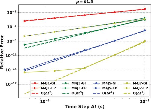
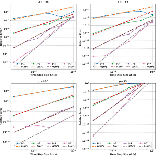
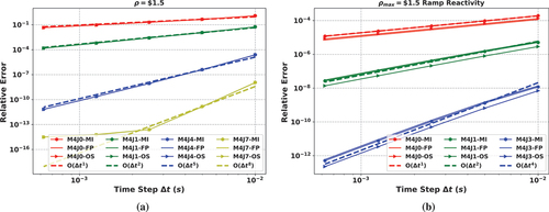
The SDC method is further verified in PKE problems with different reactivity insertions. These results are shown in Fig. 4. It can be seen that the desired order of convergence $(2M,J+1)$ is observed. Further, using a 1-ms step size for SDC achieves reasonably accurate results. Some curves are observed to deviate from the expected orders when the time step size is large. The reason for this is that the order of convergence is an asymptotic behavior, and these time steps are outside the asymptotic regime. Last, the error does not go below ${10}^{-16}$ due to machine precision of floating point arithmetic.

Fig. 4. Order of convergence of the SDC method for the PKE with different reactivities. GI is used for the residual at the right endpoint. $M$ is 4. The dashed line is the plot of the expected order of accuracy. It can be seen that the observed rate of convergence is around $J+1$.

IV.B. Stability Region

The $A$-stability investigation of the SDC method is performed for the problem

$y{ }^{\mathrm{\prime }}=-\lambda y,\lambda <0$

and

(80) $y(0)=1.$(80)

In this analysis, we suppose that the method performs a single step with step size $h$. Defining $z=\lambda h$, the value of $y$ at the next step is a function of $z$ and is denoted as $g(z)$. If $|g(z)|<1$ for $\mathrm{R}\mathrm{e}(z)<0$, then the method is $A$-stable. If $|g(z)|<1$ for $\pi -\alpha <arg(z)<\pi +\alpha$, the method is $A$-$(\alpha )$ stable. It is well known that BE is stable, but more specifically, this notion of stability is the $A$-stability.

The stability regions of SDC based on BE with EP and GI are shown in Fig. 5. They are the regions outside the lines. It can be seen that SDC is $A$-$(\alpha )$ stable for all the orders of accuracy investigated here. The approach to evaluating the endpoint value is also observed to affect the stability region. Using GI to calculate the endpoint value can make SDC $A$-stable for orders up to eight. Here for the $\mathrm{M}$-th order accurate SDC, the number of nodes used for EP is $M$ and $M/2$ for GI.

Fig. 5. Stability region of SDC: $|g(z)|<1$ for $z$ outside the lines. All the methods are $A$-$(\alpha )$ stable. They represent the results for fourth, sixth, eighth, tenth, and twelfth order SDC. For SDC with GI for the endpoint evaluation, it can be $A$-stable up to the eighth order. $J=M-1$, so $M$ is the order of accuracy.

The results presented here verify that SDC can be stable for very large orders. It turns out the SDC method can be $A$-$(\alpha )$ stable for orders up to 20. More details about the stability of SDC can be found in Refs. 10 and 11.

IV.C. Effect of Low-Order Solver

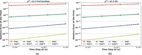
Figure 6 shows how the low-order solvers in Sec. III.A affect the performance of the SDC method for the PKE. Slight differences in the relative error can be observed. However, the order of convergence of the error does not really depend on the low-order solvers investigated here. For each method, MI, OS, and FP, the order of accuracy observed is $min(2M,J+1)$. Additionally, no instability was observed for the eighth-order accurate implementation regardless of the formulation. Thus in using SDC, the time-integration scheme can be relatively simplistic and need not require matrix inversions or analytic precursor integration to achieve notably better accuracy or stability. Consequently, the results show that SDC is a powerful approach to transform a low-order time-integration scheme into a high-order method with minimal complexity and without sacrificing stability.

Fig. 6. Effect of the low-order solvers for SDC on order of convergence: (a) simulates the PKE problem with a step reactivity insertion of 1.5 $ for 0.4 s. The reactivity simulated in (b) increases linearly from 0 to 1.5 $ in 0.4 s. Low-order solvers have a minor effect on the accuracy of SDC, but do not affect the overall order of accuracy. The dashed line is the plot of the expected order of accuracy.

Currently, the FP or SP integration technique is used to approximate the fission source in transient problems to fully couple the flux/power to the precursors.²⁶ Figure 6 also illustrates that though some improvements can be obtained by using FP compared to OS and MI, we did not observe significant improvements when SDC was used. In fact, the error from using OS was slightly smaller. The results here indicate that in the near future, numerical methods for the time-dependent Neutron Transport Equation (NTE) may be developed based on the partitioned SDC method, and the complexity from precursor integration could be avoided. This feature should be particularly important when considering the problem of precursor drift in liquid-fueled systems where an advection term is also present in Eq. (2)(2) $\begin{array}{rl}& \frac{d{\xi }_k(t)}{dt}=\frac{{\mathrm{\Lambda }}_0}{\mathrm{\Lambda }(t)}{\beta }_k(t)p(t)-{\lambda }_k(t){\xi }_k(t),k=1,2,\cdots K\end{array},$(2) .

IV.D. PKE-EF Problems

The algorithm for solving the PKE-EF problem is similar to that shown in Algorithm 2, but is omitted here for brevity. For a problem with ${\rho }^{ex}=1.5\mathrm{\$}$, ${\lambda }_H=$ 0.5/s, ${\gamma }_d=-0.8\text{rdollar}/fp\cdot s$, and the initial condition $p(0)={10}^{-4}$ fp, the effect of the number of corrections is shown in Fig. 7.

Fig. 7. Convergence study of a PKE-EF solver based on SDC. The dashed line is the plot of the expected order of accuracy. It can be seen that the order of accuracy is around $J+1$: (a) uses the full Jacobian method to calculate the error of the power and (b) uses the OS method for the error of the power.

The transient process is simulated for 0.188 s, and the relative error is calculated at 0.09 s, which is close to the peak. The reference solution is obtained with 5000 time steps with $M=5$ and $J=10$. It can be seen that the order of the accuracy is again ~J + 1, and agrees with the theoretical predictions in Ref. 11. Since the problem is solved with the SDC method based on an IMEX treatment, the SDC method is denoted as SDC-IMEX. We also observe that using the OS method to calculate the error for the PKE part is close to the full Jacobian method, which accounts for the error from the energy feedback. Therefore, we conclude that little improvement was obtained by using the Jacobian for calculating the error in the nonlinear point reactor problem. This is understandable since the major parts of the error are still from the power not from the energy feedback.

Furthermore, we do see that high-order accuracy can be achieved. The results imply that it is possible to develop the SDC for simulating the time-dependent reactor physics problem with feedback, and suggest that it is likely the methodology is extensible to spatial kinetics diffusion or transport.

IV.E. EPKEs in the TML Method

Following the verification of the accuracy of the SDC solver for the simpler problems, we turn to applying the SDC method in VERA-CS/MPACT (Ref. 18) to solve the EPKE. We do not use the SDC for the method of characteristics or coarse-mesh finite difference levels. Exactly how to extend the SDC to a multilevel transient methodology will be future work. For now, two problems are investigated. One is a single pin test problem and the other is the VERA 4-mini test problem.

The single pin test problem was developed based on the VERA core physics progression problem 1 in Ref. 29. The fuel material is initially UO₂ with 3.1% enrichment. When the transient problem is simulated with TH, the rated power of the fuel is 179 W, and the initial power is 100% fp. The simplified TH model³⁰ was used to model feedback. The transient process started with changing the enrichment from 3.1% to 3.3% in 0.025 s. This introduced a maximum reactivity of 1.98 $. Although this problem is quite contrived, it represents a very simple way to examine a super-prompt critical transient.

The 4-mini test problem is a three-dimensional regression test problem in MPACT used to verify the implementation of transient methods. The problem has the same layout as the VERA progression problem 4 (P4) (Ref. 29), but uses 7 × 7 assemblies and a shorter core. The core geometry is shown in Fig. 8a. The assemblies in red are the regions with 2.11% enriched UO₂ and the assemblies in green are the regions with 2.6% enriched UO₂ with four Pyrex rods inserted. The corner red assemblies contain four stainless steel rods inserted in the empty guide tube locations. The hybrid AIC/B₄C rod cluster control assembly (RCCA) is located in the center assembly. Unless specified, the composition of the materials and the state variables (inlet temperature, boron concentration, etc.) used in the 4-mini test problem were the same as those used in P4. Compared to P4, the height of the 4-mini test problem was reduced. The fuel stack was adjusted to be 209.16 cm rather than 365.76 cm in P4. The poison height of the AgInCd (AIC) and B₄C was adjusted to be 58.024 and 147.96 cm. The rated power was 19.36 MW, and the rated flow was 131.16 kg/s. This preserved the rated power and flow of the full core in the reduced geometry.

Fig. 8. Assembly layout and geometry of the 4-mini test problem: (a) shows the assembly, control rod bank, and poison of the problem, and (b) shows the geometry of the 4-mini test problem.

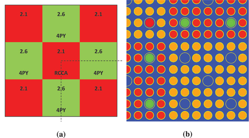
The cross sections came from the default MPACT library with 51 energy groups,³¹ and the model used heterogeneous geometry and microscopic cross sections that explicitly account for inline temperature feedback and spatially dependent resonance self-shielding.

For the initial condition, the RCCA was fully inserted. The transient case used the hot zero-power (HZP) initial condition and was simulated for 1.0 s, with RCCA withdrawn out of core over a distance of 36.27 cm in 0.05 s. The initial power of the case was 0.0136% of the rated power. More details on the problem and calculation can be found in Ref. 3.

The time step size of the SDC solver was 1 ms with $M=10$ and $J=4$. $M=10$ was used because the number of EPKE steps for TML is 10 (Refs. 2 and 3). $J=4$ was used because the SDC solver is fifth-order accurate in this case, and the results from Fig. 6 show a maximum relative error of ${10}^{-10}$, which is sufficiently accurate.

We adopted the GI for calculating the residual at the endpoint of the correction step and FP as the low-order solver. The results of the existing MPACT implementation with the BE solver were compared to the results of the SDC solver. The results from MPACT are shown in Fig. 9. Refining the time step size for the BE solver to 1 µs gave results that were comparable to the SDC results. Therefore, the implementation of SDC in MPACT is verified. When the default of 0.1 ms was used for the solution of a pin cell transient problem with a maximum reactivity of 1.98 $ using BE, it can be seen that the current BE solver with the default time step size had a maximum relative error of about 6%.

Fig. 9. Comparison of results for EPKE solvers based on BE to SDC reference in MPACT. $\mathrm{\Delta }t$ is the time step size used for the BE solver, (a) is a pin transient problem with a maximum reactivity of 1.98 $, and (b) is the 4-mini HZP problem.

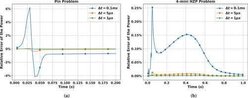
On the contrary, the SDC solver was much more accurate. Therefore, in the application of TML (Refs. 2 and 3), there is no longer a need to specify the number of EPKE steps.

It should be noted that we did not show the run-time results for these cases. The reason is that the total computational time of the EPKE solver was generally very small. It was around several seconds and was negligible compared to the run time of the transient calculation. A detailed analysis of the computational cost is shown in Sec. IV.F.

IV.F. Memory Cost and Efficiency Analysis

So far, the high-order accuracy of SDC for the linear PKE problems and the nonlinear PKE problems with feedback has been shown. In the following sections, the memory requirements and the computational cost of the SDC method are investigated.

IV.F.1. Memory Cost

Generally speaking, the memory cost of a high-order method is proportional to the order of accuracy. However, the memory cost of the SDC method is mainly determined by the number of quadrature nodes.

For the SDC method, the residual matrix $\sigma$, the derivative matrix $F$, and the solution matrix $\bar{\mathrm{\Psi }}$ are stored. Meanwhile, the integration matrix $S$ needs to be stored. Assume the solution vector is length $N$ and the number of Gauss-Legendre quadrature nodes is $M$. The memory cost for storing the residual matrix, derivative matrix, and the solution matrix is $O(MN)$. The memory cost of the integration matrix $S$ is $O(M^2)$. Therefore, the overall cost is $O(M^2+3MN)$. It should be noted that if $N$ is large, then the memory cost would be $O(3MN)$, as $M$ is very small.

For comparison, we also provide a rough estimation of the memory cost of the explicit RK methods and linear multistep methods. For the explicit P-th order RK methods of stage $s$, we know that the solution process is determined by

(81a) $y_{n+1}=y_n+h\sum i=1s{b}_i{k}_i,$(81a)

where

(81b) $k_1=f\left(t_n,y_n\right),$(81b)

(81c) $k_2=f\left(t_n+c_{2}h,y_n+h\left(a_{21}{k}_1\right)\right),$(81c)

(81d) $k_3=f\left(t_n+c_{3}h,y_n+h\left(a_{31}{k}_1+a_{32}{k}_2\right)\right),$(81d)

(81e) $⋮,$(81e)

and

(81f) $k_s=f\left(t_n+c_{s}h,y_n+h\left(a_{s1}{k}_1+a_{s2}{k}_2+\cdots +a_{s,s-1}{k}_{s-1}\right)\right).$(81f)

Therefore, the major memory cost is to store $k_i$, and the memory cost is $O(sN+s^2)$; the memory cost would be of $O(sN)$ if $N$ is large.

For a multistep method, the solution process is determined by

(82) $\sum _{j=0}^p{a}_j{y}_{n+j}=h\sum _{j=0}^p{b}_{j}f\left(t_{n+j},y_{n+j}\right).$(82)

The memory space of $O(2(p+1)N)$ should be allocated for $\{y_{n+j}\}$ and $\{f(t_{n+j},y_{n+j})\}$. Some coefficients in $\{a_j\}$ and $\{b_j\}$ can be zero. For example, for the BDF methods, all the elements of $\{a_j\}$ except $j=P$ are zero. Therefore, the additional memory is $O(pN)$.

We expect that the memory usage of the SDC method with $M$ nodes is higher than that of the explicit RK methods with $s=M$ and the linear multistep methods with $p=M$ because the residual matrix also needs to be stored. However, the memory usage of SDC will never become an issue for the PKE problem as $N$ is very small.

It should be noted that the memory cost for solving the low-order problem of SDC and for solving the linear multistep is not considered here. Considering these factors would make the analysis more complicated and beyond the scope of this work. For example, for the practical large-scaled transient problem, when the method is implicit, the Krylov subspace may be formulated when inverting a matrix is needed. The memory cost for the Krylov subspace method varies but is quite likely to be larger than that for storing the solutions and the time derivatives.

IV.F.2. Efficiency Analysis

In this section, the SDC results are compared to the results of the popular fourth-order RK method (RK4), which has four stages, to show that the SDC method can be more efficient when highly accurate results are desired. The SDC solver utilizes a Gauss-Legendre quadrature with four nodes. It can have at most eighth-order accuracy. To obtain accurate run-time results, the solvers are implemented in Fortran.

To start with, we provide a rough theoretical estimation of the computational cost of the SDC solver compared to the RK4 solver for each time step. Let the computational cost of the low-order solver be $c_l$. The computational cost of the SDC solver for low-order solution with $M$ quadrature points, $J$ corrections, and with Gauss integration for the right endpoint treatment is roughly estimated by

(83) $C_L=c_l(M+1)(J+1),$(83)

where $C_L$ is the total computational cost for the low-order solver, i.e., Euler solver. However, the derivative calculation and the spectral integration also contribute to the total computational cost. Let the computational cost of the derivative evaluation be $c_d$. Then the total computational cost for the derivation is

(84) $C_d=c_{d}MJ,$(84)

and the total computational cost for the spectral integration is

(85) $C_s=c_{s}J,$(85)

where the computational cost of a spectral integration is $c_s$. Therefore, the total computational cost is

(86) $C_T(SDC)=c_l(M+1)(J+1)+c_{d}MJ+c_{s}J.$(86)

For an implicit method, the overall computational cost should be dominated by $C_L$. However, since the PKE problem is very small, all three effects should be accounted for.

The RK4 method is based on the FE solver, which is dominated by the evaluation of the derivative. Then the overall computational cost is calculated by

(87) $C_T(RK4)=4c_d.$(87)

Therefore, we can expect that the ratio of the run time of the SDC solver to that of the RK4 solver with the same step size is

(88) $r=\frac{C_T(SDC)}{C_T(RK4)}=\frac{MJ}{4}+\frac{c_l}{c_d}\frac{(M+1)(J+1)}{4}+\frac{c_s}{c_d}\frac{J}{4}.$(88)

In general, $c_l$ should be larger than $c_d$. For the fourth-order SDC (M4J3), we have

(89) $r=\frac{12}{4}+\frac{c_l}{c_d}5+\frac{c_s}{c_d}\ge 8.$(89)

A detailed comparison for the actual run time for a subprompt problem with 0.8 $ simulated with $\mathrm{\Delta }t=0.0125$ s is shown in Table II. Compared to the RK4 solver, the fourth-order explicit SDC solver takes 15 times more. Excluding the run time of spectral integration, the fourth-order explicit SDC solver takes eight times more than RK4, which is close to the prediction of Eq. (89)(89) $r=\frac{12}{4}+\frac{c_l}{c_d}5+\frac{c_s}{c_d}\ge 8.$(89) . Therefore, for this small-sized problem, the evaluation of spectral integration makes SDC less efficient. Compared to the RK4, the SDC M4J3 reduces the error by a factor of 19. Therefore, the fourth-order SDC was not as efficient as RK4 because refining the time step size of RK4 by 15 times, RK4 can reduce the error by around a factor of 5000 (${15}^4-1\approx 5000$). The implicit SDC solver is less efficient by a large factor and takes 25 times more run time compared to the RK4.

TABLE II Run Time and Relative Error of Different Solvers for the PKE Problem with $\rho =0.8\mathrm{\$}$ for 10s with $\mathrm{\Delta }t=$ 0.0125 s

	RK4	SDC-M4J3-Explicit	SDC-M4J7-Explicit	SDC-M4J3-Implicit	SDC-M4J7-Implicit
Total run time (ms)	0.13	1.8	3.37	2.3	4.3
Spectral integration run time (ms)	0	$0.7$
Relative error	$6.4\times {10}^{-9}$	$3.4\times {10}^{-10}$	$3.4\times {10}^{-10}$	$3.8\times {10}^{-15}$	$4.2\times {10}^{-15}$

Figure 10a shows the relative error results as a function of time step size. It can be seen that the RK4 solution diverges when the time step size is larger than 50 ms. The explicit SDC results are also illustrated in Fig. 10a. The explicit SDC is also unstable when the time step size is larger than 80 ms. The implicit SDC presented in this paper is more stable with a time step size smaller than 0.5 s. The eighth-order SDC (M4J7) solver can be highly accurate; the error reaches machine precision when the time step size is smaller than 50 ms.

Fig. 10. Comparison of results for PKE solvers based on RK4 to SDC for a PKE problem with $\rho =0.8\mathrm{\$}$ for 10s. The reference results for the relative error are calculated by Matlab with analytical expression; (a) shows the relative error as a function of the time step size, and (b) shows the relative error as a function of the actual run time. “Imp” stands for implicit and “Exp” stands for explicit.

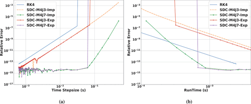
The advantage of the SDC solver is that its accuracy can be readily improved by increasing the number of corrections. Therefore, it can be observed in Fig. 10b that the SDC method is superior in achieving highly accurate results. Due to the limitations of the explicit solver, the explicit eighth-order SDC is only more efficient if it is used to obtain a result with machine precision. The implicit implementation that is investigated in this paper is more efficient for obtaining results with a relative error less than ${10}^{-10}$.

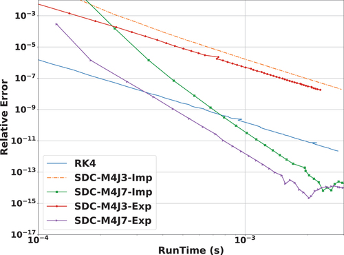
Figure 11 shows the relative error as a function of run time for another PKE problem with $\rho =1.1\mathrm{\$}$ simulated for 1 s. Once again, we observe that the SDC method is more efficient for obtaining highly accurate results with high-order convergence.

Fig. 11. Comparison of RK4 to SDC in terms of the relative error versus run-time results for a PEK problem with $\rho =0.8\mathrm{\$}$ for 1 s. The reference results for the relative error are calculated by Matlab with analytical expression.

To summarize, the results in this section show that the SDC method is not as efficient as the RK4 when the solution desired is not very accurate. The SDC method can be very efficient for achieving highly accurate results.

V. CONCLUSIONS AND FUTURE WORK

The SDC method is a high-order prediction-correction method based on using spectral integration to obtain the residuals of a low-order integration method and to calculate the predicted solutions and errors.

In this paper, we presented a preliminary application of the SDC method to the PKE. The discretized PKEs were derived for several variations of the SDC method. It was then shown that the application of the SDC method results in a stable, robust, and efficient high-order time-integration method for the PKE IVP.

Different low-order methods were proposed, and the effect of the choice of the low-order method was investigated. Results suggested that an OS or IMEX method can be used for the time integration in SDC, and the more complicated precursor integration techniques can be avoided.

The implementation of the SDC method was shown to be $A$-stable for orders up to eight, and the order of accuracy was verified for PKE problems with a range of different reactivities. The SDC implementation for the nonlinear PKE-EF was also presented and verified.

A fifth-order SDC method was then implemented to solve EPKE in MPACT, where it was shown that the simple BE integrator that is currently used by MPACT requires a time step size that is 1000× finer than what is needed for SDC to achieve the same level of error in the solution.

To illustrate the efficiency of the SDC method, a detailed comparison between the SDC solver and the RK4 was performed. It was shown that the SDC solver can be more efficient when highly accurate results are obtained.

Since SDC is a method with high-order accuracy, our future work includes investigating the application of SDC for the solution of time-dependent diffusion and transport spatial kinetics problems and the depletion equations. We will continue other investigations using the SDC method together with high-order spatial discretization methods to achieve the high-order simulation for some diffusion benchmark problems with feedback.

The accuracy of the SDC method is affected by both the time step size and the number of sweeps. Therefore, SDC can be considered as a method that has a temporal $hp$-adaptivity ($h$ is for time step size and $p$ is for the correction sweeps). We feel it would also be worthwhile to explore the adaptive methodology to apply the SDC.

We also note that the high-order time-integration methods only work for the problem where the solution varies smoothly in time. Therefore, the ultimate goal in the future would be to solve the time-dependent NTE fully coupled with TH using high-order methods for both the spatial discretization and time integration in problems with a smoothly varying operator.

Acknowledgments

This research was supported by the Consortium for Advanced Simulation of Light Water Reactors (www.casl.gov), an Energy Innovation Hub (http://www.energy.gov/hubs) for Modeling and Simulation of Nuclear Reactors under the U.S. Department of Energy contract no. DE-AC05-00OR22725. This work was also partially supported by the U.S Nuclear Regulatory Commission Faculty Development grant no. 31310019M0005.

Disclosure Statement

No potential conflict of interest was reported by the authors.

References

- A. J. HOFFMAN, “A Time-Dependent Method of Characteristics Formulation with Time Derivative Propagation,” PhD Thesis, Nuclear Engineering & Radiological Sciences University of Michigan.
- A. ZHU, Y. XU, and T. DOWNAR, “A Multilevel Quasi-Static Kinetics Method for Pin-Resolved Transport Transient Reactor Analysis,” Nucl. Sci. Eng., 182, 4, 435 (2016); https://doi.org/10.13182/NSE15-39.
- Q. SHEN et al., “Transient Multilevel Scheme with One-Group CMFD Acceleration,” Nucl. Sci. Eng., 195, 7, 741 (2021); https://doi.org/10.1080/00295639.2020.1866388.
- T. Downar, Y. Xu, and V. Seker, “PARCS v3. 0 U.S. NRC Core Neutronics Simulator Theory Manual,” University of Michigan, Department of Nuclear Engineering and Radiological Sciences (2009).
- Y. BAN, T. ENDO, and A. YAMAMOTO, “A Unified Approach for Numerical Calculation of Space-Dependent Kinetic Equation,” J. Nucl. Sci. Technol., 49, 5, 496 (2012); https://doi.org/10.1080/00223131.2012.677126.
- J.-Y. CHO et al., “Transient Capability for a MOC-Based Whole Core Transport Code DeCART,” Trans. Am. Nucl. Soc., p. 2, American Nuclear Society 92, 721–722 (2015).
- C. B. SHIM et al., “Application of Backward Differentiation Formula to Spatial Reactor Kinetics Calculation with Adaptive Time Step Control,” Nucl. Eng. Technol., 43 6, 16 (2011).
- Z. ZHANG and Y. CAI, “A Numerical Solution to the Point Kinetic Equations Using Diagonally Implicit Runge Kutta Method,” Proc. Int. Conf. on Nuclear Engineering, p. V001T02A001, American Society of Mechanical Engineers (2016); https://doi.org/10.1115/ICONE24-60011.
- A. J. HOFFMAN and J. C. LEE, “A Time-Dependent Neutron Transport Method of Characteristics Formulation with Time Derivative Propagation,” J. Comput. Phys., 306, 696, (2016) https://doi.org/10.1016/j.jcp.2015.10.039.
- D. BEYLKIN, “Spectral Deferred Corrections for Parabolic Partial Differential Equations,” Technical Report, Yale University (2015).
- A. DUTT, L. GREENGARD, and V. ROKHLIN, “Spectral Deferred Correction Methods for Ordinary Differential Equations,” BIT Numer. Math., 40, 2, 241 (2000); https://doi.org/10.1023/A:1022338906936.
- K. BÖHMER and H. STETTER, Defect Correction Methods, Vol. 5 of Computing Supplementum, Springer (1984); https://doi.org/10.1007/978-3-7091-7023-6.
- Y. CAI et al., “Parallel Computation of the Point Neutron Kinetic Equations Using Parallel Revisionist Integral Deferred Correction,” Proc. 2018 26th Int. Conf. on Nuclear Engineering, p. V003T02A010, American Society of Mechanical Engineers, London, England (2018); https://doi.org/10.1115/ICONE26-81205.
- Y. CAI, Q. LI, and K. WANG, “A Numerical Solution to the Point Kinetic Equations Using Spectral Deferred Correction,” Trans. Am. Nucl. Soc., 111, 734 (2014).
- M. L. MINION, “Semi-implicit Spectral Deferred Correction Methods for Ordinary Differential Equations,” Commun. Math. Sci., 1, 3, 471 (2003); https://doi.org/10.4310/cms.2003.v1.n3.a6.
- M. M. CROCKATT et al., “An Arbitrary-Order, Fully Implicit, Hybrid Kinetic Solver for Linear Radiative Transport Using Integral Deferred Correction,” J. Comput. Phys., 346, 212 (2017); https://doi.org/10.1016/j.jcp.2017.06.017.
- D. Z. HUANG et al., “High-Order Partitioned Spectral Deferred Correction Solvers for Multiphysics Problems,” J. Comput. Phys., 412, 109441 (2020); https://doi.org/10.1016/j.jcp.2020.109441.
- B. KOCHUNAS et al., “VERA Core Simulator Methodology for Pressurized Water Reactor Cycle Depletion,” Nucl. Sci. Eng., 185, 1, 217 (2017); https://doi.org/10.13182/NSE16-39.
- K. O. OTT and R. J. NEUHOLD, Introductory Nuclear Reactor Dynamics, American Nuclear Society, (1985).
- Q. SHEN, “Robust and Efficient Methods in Transient Whole-Core Neutron Transport Calculations,” PhD Thesis, Nuclear Engineering & Radiological Sciences University of Michigan (2021).
- H. FINNEMANN and A. GALATI, “NEACRP 3-D LWR Core Transient Benchmark,” Technical Report NEACRP-L-355, Nuclear Energy Agency (Jan. 1992).
- L. GREENGARD, “Spectral Integration and Two-Point Boundary Value Problems,” SIAM J. Numer. Anal., 28, 4, 1071 (1991); https://doi.org/10.1137/0728057.
- M. F. CAUSLEY and D. C. SEAL, “On the Convergence of Spectral Deferred Correction Methods,” Commun. Appl. Math. Comput. Sci, 14, 1, 33 (2019); https://doi.org/10.2140/CAMCOS.2019.14.33.
- M. MINION, “A Hybrid Parareal Spectral Deferred Corrections Method,” Commun. Appl. Math. Comput. Sci, 5, 2, 265 (2011); https://doi.org/10.2140/camcos.2010.5.265.
- R. SPECK et al., “A Multi-level Spectral Deferred Correction Method,” BIT Numer. Math, 55, 3, 843 (2015); https://doi.org/10.1007/s10543-014-0517-x.
- A. ZHU, “Transient Methods for Pin-Resolved Whole-Core Neutron Transport,” PhD Thesis, Nuclear Engineering & Radiological Sciences University of Michigan (2016).
- T. HAGSTROM and R. ZHOU, “On the Spectral Deferred Correction of Splitting Methods for Initial Value Problems,” Commun. Appl. Math. Comput. Sci, 1, 1, 169 (2006); https://doi.org/10.2140/camcos.2006.1.169.
- J. HUANG, J. JIA, and M. MINION, “Accelerating the Convergence of Spectral Deferred Correction Methods,” J. Comput. Phys., 214, 2, 633 (2006); https://doi.org/10.1016/j.jcp.2005.10.004.
- A. T. GODFREY, “VERA Core Physics Benchmark Progression Problem Specifications,” Technical Report 793, Consortium for Advanced Simulation of Light Water Reactors (2014).
- A. GRAHAM et al., “Assessment of Thermal-Hydraulic Feedback Models,” Proc. PHYSOR 2016: Unifying Theory and Experiments in the 21st Century, 6, 3616, Sun Valley, Idaho (2016).
- K. S. KIM et al., “Development of the Multigroup Cross Section Library for the CASL Neutronics Simulator MPACT: Verification,” Ann. Nucl. Energy, 132, 1 (2019); https://doi.org/10.1016/j.anucene.2019.03.041.