Space-Dependent Calculation of the Multiplicity Moments for Shells With the Inclusion of Scattering

Abstract

In recent work, we extended the methodology of multiplicity counting in nuclear safeguards by elaborating the one-speed stochastic transport theory of the calculation of the so-called multiplicity moments, i.e., the factorial moments of the number of neutrons emitted from a fissile item, following a source event from an internal neutron source [spontaneous fission and ($\alpha ,n$) reactions]. Calculations were made for solid spheres and cylinders, with the source being homogeneously distributed within the item. Recent measurements of the Rocky Flats Shells during the Measurement of Uranium Subcritical and Critical (MUSIC) campaign conducted by Los Alamos National Laboratory and assisted by the University of Michigan inspired us to extend the model to spherical shell geometry with a point source in the middle of the central cavity. Comparison of the calculated results with the experimental ones indicated that accounting for fission as the only neutron reaction (the standard procedure in the point model, adapted also in our work so far) was not sufficient for reaching good agreement with measurements. The model was therefore extended to include elastic scattering into the one-speed formalism, whereas the effect of inelastic scattering was accounted for in an empirical way. After these extensions, good agreement was found between the calculated and the measured values. The paper describes the extension of the theory and provides concrete quantitative results.

Keywords:

• Multiplicity moments
• space-dependent model
• shell items
• point source
• elastic scattering
• inelastic scattering
• Rocky Flats Shells

I. INTRODUCTION

Determining the parameters of an unknown sample, primarily the fission rate, which is proportional to the mass of the even number isotope, with passive interrogation methods is based on multiplicity counting. This is achieved by measurement of the rate of single neutron detections as well as the rate of detecting neutrons in double and triple coincidences (the singles, doubles, and triples rates). These, in turn, depend on the factorial moments of the number of neutrons emitted from a fissile sample following a source emission event (also referred to as multiplicity moments or just “Böhnel moments”)¹. These moments depend on the parameters of the sample in which one is interested; hence, an expression of these moments as functions of the sample parameters make it possible to determine the sought parameters from the measured multiplicity moments by an inversion of the expressions.

In the traditional method used so far, these multiplicity moments are derived theoretically in the so-called point model, in which the spatial and angular dependence of the neutrons inside the sample is neglected; only the number distribution of the neutron emission by the internal source and the internal multiplication within the sample by a uniform first collision probability are accounted for.¹ By neglecting the spatial and angular aspects of neutron transport inside a finite item with given boundary conditions, the point model is clearly only an approximation/simplification of the real case and will not be able to reconstruct the multiplicity moments exactly. This means that the usual method of unfolding the fission rate of the unknown sample from the measured multiplicity moments based on the point model formulas will lead to a biased value. A more realistic and better method of calculating the multiplicity moments, which accounts for the spatial and angular transport of neutrons in the finite item, would increase the accuracy of the identification of the sample mass.

In recent publications, we introduced a method for the calculation of the multiplicity moments beyond the point model, i.e., in a one-speed transport theory model, in which the spatial and angular transport of the neutrons is taken into account.^2–4 A general theory was developed for the calculation of the moments in arbitrary geometries for solid, homogeneous items. Concrete calculations were made for items with spherical and cylindrical geometries with a collision number expansion. Because of the symmetry properties of these shapes, the calculations were simplified as compared to an arbitrary geometry.

One limitation of the previous work, even at the level of the general theory, was that it was formulated for cases where the item was homogeneous, the internal source was distributed evenly and homogeneously inside the item, and the angular distribution of the source neutrons was isotropic. Recently, a need arose to relax these limitations in connection with an ongoing project related to the Measurement of Uranium Subcritical and Critical (MUSIC) experimental measurements campaign.^5–7 The campaign consisted of measurements on the Rocky Flats Shells (stacked shells of highly enriched metallic uranium, consisting of 93% ²³⁵U; see Refs. 7 and 8) driven by a ²⁵²Cf point source placed in the center of each configuration. This measuring arrangement is equivalent to a spherical shell having a central spherical cavity, a point source in the center, but no source distributed in the fissile part.

In order that such a case be treated, extension of the theory is needed in several points. One is treatment of the central cavity, which means that the item is not uniform and homogeneous. Neutrons entering the cavity will travel through it without collisions. In other words, the reaction cross sections are not constant in space any longer. This fact affects the equations for single particle–induced distribution, which is the first step when backward master equations are used. Another is that the source is not homogeneous in space either. This affects the equation connecting the single particle induced–distribution, and hence its moments, to the source-induced distribution and its moments.⁹ Treatment of point sources in neutron transport is a standard procedure, although a point source in the center of the cavity requires some care.

With the model extended to shells with a point source in the center of the cavity, preliminary calculations were made with data of the Rocky Flats Shells. Comparison with the measurements showed that the calculated moments were systematically lower than the measured ones. Calculation of the critical sizes of pure ²³⁵U and ²³⁹Pu samples and comparison with known criticality data also showed that the model underestimates the internal multiplication in the item. To improve the accuracy of the predictions, the effect of elastic scattering was included in the model. This led to a significant, but still not fully satisfactory, improvement with regard to both the comparison with the measurements on the Rocky Flats Shells and the comparison with critical sizes. To improve the agreement further, the effect of inelastic scattering was accounted for in an approximate manner with a phenomenological method such that the one-speed character of the model could still be kept.

With these extensions, rather good agreement was found between the calculated and the measured data for the Rocky Flats Shells. In the following, these extensions will be described one after the other, and quantitative values of the calculations will be given.

II. TREATMENT OF THE CAVITY

Since the central spherical cavity does not affect the spherical symmetry, in this piece of work for the treatment of the item with a nonhomogeneous material distribution, we will use the spherical geometry model of Ref. 3 as the starting point. Also, since we want to model the case of a spontaneous fission source with a pure metallic uranium sample, the $\alpha$ factor will be taken as zero throughout. Including a nonzero $\alpha$ factor is a matter of triviality since it requires only the rescaling of the probability distribution of the source neutrons.^1,10

Since the multiplicity moments, even in the point model, are described by backward-type master equations, one needs first an equation for the number distribution of the emitted neutrons due to one starting particle.^a Then, another equation is needed to connect the distribution (or its generating function) of the single particle–induced event with that of the case starting with a source emission event (a random number of particles starting the process). The presence of the cavity affects primarily the single particle–induced distribution; hence, in this section, only this will be treated. The relationship between the single neutron–induced and source event–induced distributions will be treated in connection with the point source; Sec. III.

In Refs. 2 and 3, assuming a homogeneous sphere of radius $R$ and that the induced fission neutrons have an isotropic angular distribution, the following master equation was derived for the distribution $p(\mathbf{n}=n|r,\mu )\equiv p(n|r,\mu )$ of emission of a total number of $n$ neutrons, due to one starting neutron at radial position $r$ and directional cosine $\mu$ with respect to the position vector:

(1) $\begin{array}{rl}& p(n|r,\mu )=e^{-\mathrm{\ell }(r,\mu ){\mathrm{\Sigma }}_f}{\delta }_{n,1}+{\mathrm{\Sigma }}_f{\int }_0^{\mathrm{\ell }(r,\mu )}ds{e}^{-s{\mathrm{\Sigma }}_f}\sum _0^{\mathrm{\infty }}{p}_r(k)\sum _{n_1+n_2+\dots +n_k=n}{\int }_{-1}^1\frac{d{\mu }_1}{2}\frac{d{\mu }_2}{2}\dots \frac{d{\mu }_k}{2}\\ & \times p(n_1|r^{\prime }(s),{\mu }_1)p(n_2|r^{\prime }(s),{\mu }_2)\dots p(n_k|r^{\prime }(s),{\mu }_k).\end{array}$(1)

Introducing the generating function $g(z|r,\mu )$ of $p(n|r,\mu )$ as

(2) $g(z|r,\mu )=\sum _{n=0}^{\mathrm{\infty }}{z}^{n}p(n|r,\mu )$(2)

and switching to optical units (distances measured in units of the mean free path), one obtains a substantially simpler equation for the generating function in the form

(3) $g(z|r,\mu )=z{e}^{-\mathrm{\ell }(r,\mu )}+{\int }_0^{\mathrm{\ell }(r,\mu )}ds{e}^{-s}{q}_r\left[g(z|r{ }^{\mathrm{\prime }}(s))\right].$(3)

In the above, $\mathbf{n}$ is a random variable and $n$ is a realization of it, $q_r$ is the generating function of the number distribution of the induced fission neutrons,

(4) $g(z|r)=\frac{1}{2}{\int }_{-1}^{1}d\mu g(z|r,\mu )$(4)

is the “scalar” generating function,

(5) $r{ }^{\mathrm{\prime }}(s)=\sqrt{r^2+s^2+2rs\mu }$(5)

is the radial position of the neutron at a distance $s$ away from the starting point $r$ along direction $\mu$, and

(6) $\mathrm{\ell }(r,\mu )=-r\mu +\sqrt{{(r\mu )}^2+(R^2-r^2)}=-r\mu +\sqrt{r^2({\mu }^2-1)+R^2}$(6)

is the distance to the boundary of the sphere of radius $R$ from radial position $r$ along direction $\mu$, the latter being the polar angle between the neutron position vector at the starting point and the neutron velocity vector. Here, all distance units are measured in dimensionless optical path units, i.e., units of the mean free path $1/{\mathrm{\Sigma }}_f$ (the only reaction is assumed to be fission). The use of the optical path in the equations simplifies the notations and makes the formalism more transparent.

To apply the same equation for a shell with a central cavity of radius $r_0$, the expressions for the solid sphere are modified as follows. As is illustrated in Fig. 1, for each radial starting position $r,$ there is a critical polar angle, with a corresponding ${\mu }_{cr}$, equal to

(7) ${\mu }_{cr}(r)\equiv {\mu }_{cr}=-\sqrt{1-\frac{r_0^2}{r^2}}\le 0,$(7)

Fig. 1. Illustration of the neutron paths for $\mu >{\mu }_{cr}$ and for $\mu <{\mu }_{cr}$ in the shell with a central cavity.

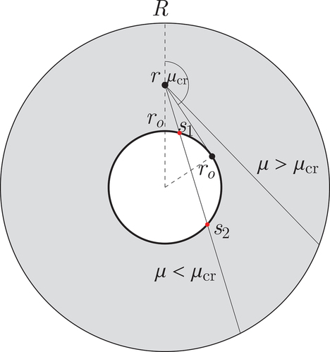
which separates the trajectories into two classes. Neutrons starting from a point $r$ with

(8) $\mu \ge {\mu }_{cr}$(8)

will not pass the cavity; hence, the distance $\mathrm{\ell }(r,\mu )$ to the boundary from point $r$ into direction cosine $\mu$ has to be calculated exactly as before, whereas neutrons with

(9) $\mu <{\mu }_{cr}$(9)

will have part of their trajectory in the cavity, where no reactions can take place. This is the section of the path between the points $s_1$ and $s_2$ in Fig. 1, in terms of the path length. These points, valid only for $\mu <{\mu }_{cr}$, are given as

(10) $s_{1,2}\equiv s_{1,2}(r,\mu )=-r\mu \mp \sqrt{{(r\mu )}^2-(r^2-r_0^2)}.$(10)

One way of treating the cavity is to rewrite Eq. (3)(3) $g(z|r,\mu )=z{e}^{-\mathrm{\ell }(r,\mu )}+{\int }_0^{\mathrm{\ell }(r,\mu )}ds{e}^{-s}{q}_r\left[g(z|r{ }^{\mathrm{\prime }}(s))\right].$(3) for the single particle–induced generating function to the case where the cross section of the material is a function of space. To keep the advantages of using the optical path, corresponding to the medium, we define the normalized cross section

(11) $\sigma (r)=\frac{\mathrm{\Sigma }(r)}{{\mathrm{\Sigma }}_f},$(11)

where

(12) $\mathrm{\Sigma }(r)=\left\{\begin{array}{cc}{\mathrm{\Sigma }}_f& \mathrm{f}\mathrm{o}\mathrm{r}r\ge r_0\\ 0& \mathrm{f}\mathrm{o}\mathrm{r}r<r_0\end{array}\right.$(12)

with ${\mathrm{\Sigma }}_f$ being the constant fission cross section inside the shell. From Eqs. (11)(11) $\sigma (r)=\frac{\mathrm{\Sigma }(r)}{{\mathrm{\Sigma }}_f},$(11) and (12(12) $\mathrm{\Sigma }(r)=\left\{\begin{array}{cc}{\mathrm{\Sigma }}_f& \mathrm{f}\mathrm{o}\mathrm{r}r\ge r_0\\ 0& \mathrm{f}\mathrm{o}\mathrm{r}r<r_0\end{array}\right.$(12) ), it immediately follows that

(13) $\sigma (r)=\mathrm{\Delta }(r-r_0),$(13)

where $\mathrm{\Delta }(x)$ is the unit step function.

With the above space-dependent relative cross section, which defines a generalized optical path length, Eq. (3)(3) $g(z|r,\mu )=z{e}^{-\mathrm{\ell }(r,\mu )}+{\int }_0^{\mathrm{\ell }(r,\mu )}ds{e}^{-s}{q}_r\left[g(z|r{ }^{\mathrm{\prime }}(s))\right].$(3) will take the form

(14) $g(z|r,\mu )=z{e}^{-{\int }_0^{\mathrm{\ell }(r,\mu )}\sigma (r{ }^{\mathrm{\prime }}(s))\mathrm{d}s}+{\int }_0^{\mathrm{\ell }(r,\mu )}ds\sigma (r{ }^{\mathrm{\prime }}(s))e^{-\sigma (r{ }^{\mathrm{\prime }}(s))s}{q}_r\left[g(z|r{ }^{\mathrm{\prime }}(s))\right].$(14)

Here, in contrast to Eq. (1(1) $\begin{array}{rl}& p(n|r,\mu )=e^{-\mathrm{\ell }(r,\mu ){\mathrm{\Sigma }}_f}{\delta }_{n,1}+{\mathrm{\Sigma }}_f{\int }_0^{\mathrm{\ell }(r,\mu )}ds{e}^{-s{\mathrm{\Sigma }}_f}\sum _0^{\mathrm{\infty }}{p}_r(k)\sum _{n_1+n_2+\dots +n_k=n}{\int }_{-1}^1\frac{d{\mu }_1}{2}\frac{d{\mu }_2}{2}\dots \frac{d{\mu }_k}{2}\\ & \times p(n_1|r^{\prime }(s),{\mu }_1)p(n_2|r^{\prime }(s),{\mu }_2)\dots p(n_k|r^{\prime }(s),{\mu }_k).\end{array}$(1) ), the multiplying cross section in the second term on the right-hand side had to be moved inside the integral because the cross sections are now space dependent in order to account for the central cavity. Rewriting Eq. (13)(13) $\sigma (r)=\mathrm{\Delta }(r-r_0),$(13) in terms of the path length variable $s$ as

(15) $\sigma (s)=\left\{\begin{array}{cc}1& \mathrm{f}\mathrm{o}\mathrm{r}\mu \ge {\mu }_{cr}\\ \mathrm{\Delta }(s_1-s)+\mathrm{\Delta }(s-s_2)& \mathrm{f}\mathrm{o}\mathrm{r}\mu <{\mu }_{cr}\end{array}\right.$(15)

and substituting Eq. (15)(15) $\sigma (s)=\left\{\begin{array}{cc}1& \mathrm{f}\mathrm{o}\mathrm{r}\mu \ge {\mu }_{cr}\\ \mathrm{\Delta }(s_1-s)+\mathrm{\Delta }(s-s_2)& \mathrm{f}\mathrm{o}\mathrm{r}\mu <{\mu }_{cr}\end{array}\right.$(15) into Eq. (14)(14) $g(z|r,\mu )=z{e}^{-{\int }_0^{\mathrm{\ell }(r,\mu )}\sigma (r{ }^{\mathrm{\prime }}(s))\mathrm{d}s}+{\int }_0^{\mathrm{\ell }(r,\mu )}ds\sigma (r{ }^{\mathrm{\prime }}(s))e^{-\sigma (r{ }^{\mathrm{\prime }}(s))s}{q}_r\left[g(z|r{ }^{\mathrm{\prime }}(s))\right].$(14) leads to the equation for the single particle–induced generating function in the form

(16) $\begin{array}{c}g(z|r,\mu )=\mathrm{\Delta }(\mu -{\mu }_{cr}(r))\left\{z{e}^{-\mathrm{\ell }(r,\mu )}+{\int }_0^{\mathrm{\ell }(r,\mu )}ds{e}^{-s}{q}_r\left[g(z|r^{\prime }(s))\right]\right\}\\ +\mathrm{\Delta }({\mu }_{cr}(r)-\mu )\left\{\begin{array}{c}z{e}^{-\mathrm{\ell }(r,\mu )+(s_2(r,\mu )-s_1(r,\mu ))}+{\int }_0^{s_1(r,\mu )}ds{e}^{-s}{q}_r\left[g(z|r^{\prime }(s))\right]\end{array}\right.\\ +e^{(s_2(r,\mu )-s_1(r,\mu ))}{\int }_{s_2(r,\mu )}^{\mathrm{\ell }(r,\mu )}ds{e}^{-s}{q}_r\left[g(z|r^{\prime }(s))\right]\}.\end{array}$(16)

It is also interesting to write down the equation for the scalar (angularly integrated) generating function, from which the scalar moments can be derived. This is partly because in the Neumann-series solution, one needs only the scalar moments. Moreover, if the source is distributed in the item and is isotropic, then one actually needs only the scalar single particle–induced moments to calculate the source-induced moments. But, even if the angular moments are needed (which is the case of a source in a cavity, as we will soon see), it is still sufficient to obtain a solution for the scalar moments, from which the angularly dependent moments can be easily calculated with a simple quadrature. This will be shown explicitly below.

Therefore, for both the generating function of the single particle–induced distribution and the moments, we will also list the equations for the scalar quantities. By integrating Eq. (16)(16) $\begin{array}{c}g(z|r,\mu )=\mathrm{\Delta }(\mu -{\mu }_{cr}(r))\left\{z{e}^{-\mathrm{\ell }(r,\mu )}+{\int }_0^{\mathrm{\ell }(r,\mu )}ds{e}^{-s}{q}_r\left[g(z|r^{\prime }(s))\right]\right\}\\ +\mathrm{\Delta }({\mu }_{cr}(r)-\mu )\left\{\begin{array}{c}z{e}^{-\mathrm{\ell }(r,\mu )+(s_2(r,\mu )-s_1(r,\mu ))}+{\int }_0^{s_1(r,\mu )}ds{e}^{-s}{q}_r\left[g(z|r^{\prime }(s))\right]\end{array}\right.\\ +e^{(s_2(r,\mu )-s_1(r,\mu ))}{\int }_{s_2(r,\mu )}^{\mathrm{\ell }(r,\mu )}ds{e}^{-s}{q}_r\left[g(z|r^{\prime }(s))\right]\}.\end{array}$(16) with respect to μ, one obtains the equation for the scalar generating function as

(17) $\begin{array}{c}g(z|r)=z{g}_0(r)+\frac{1}{2}{\int }_{-1}^{{\mu }_{cr}}d\mu \left\{{\int }_0^{s_1(r,\mu )}ds{e}^{-s}{q}_r\left[g(z|r{ }^{\mathrm{\prime }}(s))\right]\right.\\ +\left.e^{[s_2(r,\mu )-s_1(r,\mu )]}{\int }_{s_2(r,\mu )}^{\mathrm{\ell }(r,\mu )}ds{e}^{-s}{q}_r\left[g(z|r{ }^{\mathrm{\prime }}(s))\right]\right\}+\frac{1}{2}{\int }_{{\mu }_{cr}}^{1}d\mu {\int }_0^{\mathrm{\ell }(r,\mu )}ds{e}^{-s}{q}_r\left[g(z|r{ }^{\mathrm{\prime }}(s))\right],\end{array}$(17)

where

(18) $g_0(r)=n_0(r)=\frac{1}{2}\left[{\int }_{-1}^{{\mu }_{cr}}d\mu e^{-[\mathrm{\ell }(r,\mu )-s_2(r,\mu )+s_1(r,\mu )]}+{\int }_{{\mu }_{cr}}^{1}d\mu e^{-\mathrm{\ell }(r,\mu )}\right].$(18)

From Eq. (16(16) $\begin{array}{c}g(z|r,\mu )=\mathrm{\Delta }(\mu -{\mu }_{cr}(r))\left\{z{e}^{-\mathrm{\ell }(r,\mu )}+{\int }_0^{\mathrm{\ell }(r,\mu )}ds{e}^{-s}{q}_r\left[g(z|r^{\prime }(s))\right]\right\}\\ +\mathrm{\Delta }({\mu }_{cr}(r)-\mu )\left\{\begin{array}{c}z{e}^{-\mathrm{\ell }(r,\mu )+(s_2(r,\mu )-s_1(r,\mu ))}+{\int }_0^{s_1(r,\mu )}ds{e}^{-s}{q}_r\left[g(z|r^{\prime }(s))\right]\end{array}\right.\\ +e^{(s_2(r,\mu )-s_1(r,\mu ))}{\int }_{s_2(r,\mu )}^{\mathrm{\ell }(r,\mu )}ds{e}^{-s}{q}_r\left[g(z|r^{\prime }(s))\right]\}.\end{array}$(16) ), equations can be derived for the angular factorial moments by successive derivation with respect to $z$. For the first moment

(19) $⟨\mathbf{n}(r,\mu )⟩\equiv n(r,\mu )={\left.\frac{\mathrm{\partial }g(z|r,\mu )}{z}\right|}_{z=1},$(19)

one obtains

(20) $\begin{array}{c}n(r,\mu )=\mathrm{\Delta }(\mu -{\mu }_{cr}(r))[e^{-\mathrm{\ell }(r,\mu )}+{\nu }_{r,1}{\int }_0^{\mathrm{\ell }(r,\mu )}ds{e}^{-s}n(r{ }^{\mathrm{\prime }}(s))]\\ +\mathrm{\Delta }({\mu }_{cr}(r)-\mu )[e^{-\mathrm{\ell }(r,\mu )+(s_2(r,\mu )-s_1(r,\mu ))}+{\nu }_{r,1}{\int }_0^{s_1(r,\mu )}ds{e}^{-s}n(r{ }^{\mathrm{\prime }}(s))\\ +{\nu }_{r,1}{e}^{[s_2(r,\mu )-s_1(r,\mu )]}{\int }_{s_2(r,\mu )}^{\mathrm{\ell }(r,\mu )}ds{e}^{-s}n(r{ }^{\mathrm{\prime }}(s))].\end{array}$(20)

From Eqs. (17)(17) $\begin{array}{c}g(z|r)=z{g}_0(r)+\frac{1}{2}{\int }_{-1}^{{\mu }_{cr}}d\mu \left\{{\int }_0^{s_1(r,\mu )}ds{e}^{-s}{q}_r\left[g(z|r{ }^{\mathrm{\prime }}(s))\right]\right.\\ +\left.e^{[s_2(r,\mu )-s_1(r,\mu )]}{\int }_{s_2(r,\mu )}^{\mathrm{\ell }(r,\mu )}ds{e}^{-s}{q}_r\left[g(z|r{ }^{\mathrm{\prime }}(s))\right]\right\}+\frac{1}{2}{\int }_{{\mu }_{cr}}^{1}d\mu {\int }_0^{\mathrm{\ell }(r,\mu )}ds{e}^{-s}{q}_r\left[g(z|r{ }^{\mathrm{\prime }}(s))\right],\end{array}$(17) and (18(18) $g_0(r)=n_0(r)=\frac{1}{2}\left[{\int }_{-1}^{{\mu }_{cr}}d\mu e^{-[\mathrm{\ell }(r,\mu )-s_2(r,\mu )+s_1(r,\mu )]}+{\int }_{{\mu }_{cr}}^{1}d\mu e^{-\mathrm{\ell }(r,\mu )}\right].$(18) ), or alternatively, angularly integrating Eq. (20(20) $\begin{array}{c}n(r,\mu )=\mathrm{\Delta }(\mu -{\mu }_{cr}(r))[e^{-\mathrm{\ell }(r,\mu )}+{\nu }_{r,1}{\int }_0^{\mathrm{\ell }(r,\mu )}ds{e}^{-s}n(r{ }^{\mathrm{\prime }}(s))]\\ +\mathrm{\Delta }({\mu }_{cr}(r)-\mu )[e^{-\mathrm{\ell }(r,\mu )+(s_2(r,\mu )-s_1(r,\mu ))}+{\nu }_{r,1}{\int }_0^{s_1(r,\mu )}ds{e}^{-s}n(r{ }^{\mathrm{\prime }}(s))\\ +{\nu }_{r,1}{e}^{[s_2(r,\mu )-s_1(r,\mu )]}{\int }_{s_2(r,\mu )}^{\mathrm{\ell }(r,\mu )}ds{e}^{-s}n(r{ }^{\mathrm{\prime }}(s))].\end{array}$(20) ), one obtains for the scalar first moment $n(r)$ the equation

(21) $\begin{array}{c}n(r)=n_0(r)+\frac{{\nu }_{r,1}}{2}\left[{\int }_{-1}^{{\mu }_{cr}}d\mu \left\{{\int }_0^{s_1(r,\mu )}ds{e}^{-s}n(r{ }^{\mathrm{\prime }}(s))\right.\right.\\ +\left.\left.e^{[s_2(r,\mu )-s_1(r,\mu )]}{\int }_{s_2(r,\mu )}^{\mathrm{\ell }(r,\mu )}ds{e}^{-s}n(r{ }^{\mathrm{\prime }}(s))\right\}+{\int }_{{\mu }_{cr}}^{1}d\mu {\int }_0^{\mathrm{\ell }(r,\mu )}ds{e}^{-s}n(r{ }^{\mathrm{\prime }}(s))\right],\end{array}$(21)

where $n_0(r)$ is defined in Eq. (18)(18) $g_0(r)=n_0(r)=\frac{1}{2}\left[{\int }_{-1}^{{\mu }_{cr}}d\mu e^{-[\mathrm{\ell }(r,\mu )-s_2(r,\mu )+s_1(r,\mu )]}+{\int }_{{\mu }_{cr}}^{1}d\mu e^{-\mathrm{\ell }(r,\mu )}\right].$(18) .

Similar equations can be derived for the second and third factorial moments $m(r,\mu )$ and $w(r,\mu )$, respectively. For the second angular moment, $⟨(\mathbf{n}(r,\mu )(\mathbf{n}(r,\mu )-1)⟩\equiv m(r,\mu ),$ one obtains

(22) $\begin{array}{c}m(r,\mu )=\mathrm{\Delta }(\mu -{\mu }_{cr}(r)){\int }_0^{\mathrm{\ell }(r,\mu )}ds{e}^{-s}\{{\nu }_{r,2}{n}^2(r{ }^{\mathrm{\prime }}(s))+{\nu }_{r,1}m(r{ }^{\mathrm{\prime }}(s))\}\\ +\mathrm{\Delta }({\mu }_{cr}(r)-\mu )[{\int }_0^{s_1(r,\mu )}ds{e}^{-s}\{{\nu }_{r,2}{n}^2(r{ }^{\mathrm{\prime }}(s))+{\nu }_{r,1}m(r{ }^{\mathrm{\prime }}(s))\}\\ +e^{(s_2(r,\mu )-s_1(r,\mu ))}{\int }_{s_2(r,\mu )}^{\mathrm{\ell }(r,\mu )}ds{e}^{-s}\{{\nu }_{r,2}{n}^2(r{ }^{\mathrm{\prime }}(s))+{\nu }_{r,1}m(r{ }^{\mathrm{\prime }}(s))]\}\end{array}$(22)

whereas for the scalar second moment, one has

(23) $\begin{array}{c}m(r)=m_0(r)+\frac{{\nu }_{r,1}}{2}\left[{\int }_{-1}^{{\mu }_{cr}}d\mu \left\{{\int }_0^{s_1(r,\mu )}ds{e}^{-s}m(r{ }^{\mathrm{\prime }}(s))\right.\right.\\ +\left.\left.e^{[s_2(r,\mu )-s_1(r,\mu )]}{\int }_{s_2(r,\mu )}^{\mathrm{\ell }(r,\mu )}ds{e}^{-s}m(r{ }^{\mathrm{\prime }}(s))\right\}+{\int }_{{\mu }_{cr}}^{1}d\mu {\int }_0^{\mathrm{\ell }(r,\mu )}ds{e}^{-s}m(r{ }^{\mathrm{\prime }}(s))\right]\end{array}$(23)

with

(24) $\begin{array}{c}{m}_0(r)=\frac{{\nu }_{r,2}}{2}\left[{\int }_{-1}^{{\mu }_{cr}}d\mu \left\{{\int }_0^{s_1(r,\mu )}ds{e}^{-s}{n}^2(r{ }^{\mathrm{\prime }}(s))\right.\right.\\ +\left.\left.e^{[s_2(r,\mu )-s_1(r,\mu )]}{\int }_{s_2(r,\mu )}^{\mathrm{\ell }(r,\mu )}ds{e}^{-s}{n}^2(r{ }^{\mathrm{\prime }}(s))\right\}+{\int }_{{\mu }_{cr}}^{1}d\mu {\int }_0^{\mathrm{\ell }(r,\mu )}ds{e}^{-s}{n}^2(r{ }^{\mathrm{\prime }}(s))\right].\end{array}$(24)

The third factorial moment, $⟨(\mathbf{n}(r,\mu )(\mathbf{n}(r,\mu )-1))(\mathbf{n}(r,\mu )-2)⟩\equiv w(r,\mu ),$ can be derived in an analogous manner. One obtains

(25) $\begin{array}{c}w(r,\mu )=\mathrm{\Delta }(\mu -{\mu }_{cr}(r)){\int }_0^{\mathrm{\ell }(r,\mu )}ds{e}^{-s}\left\{{\nu }_{r,3}{n}^3(r{ }^{\mathrm{\prime }}(s))+3{\nu }_{r,2}n(r{ }^{\mathrm{\prime }}(s))m(r{ }^{\mathrm{\prime }}(s))+{\nu }_{r,1}w(r{ }^{\mathrm{\prime }}(s))\right\}\\ +\mathrm{\Delta }({\mu }_{cr}(r)-\mu )\left[{\int }_0^{s_1(r,\mu )}ds{e}^{-s}\left\{{\nu }_{r,3}{n}^3(r{ }^{\mathrm{\prime }}(s))+3{\nu }_{r,2}n(r{ }^{\mathrm{\prime }}(s))m(r{ }^{\mathrm{\prime }}(s))+{\nu }_{r,1}w(r{ }^{\mathrm{\prime }}(s))\right\}\right.\\ \left.+e^{(s_2(r,\mu )-s_1(r,\mu ))}{\int }_{s_2(r,\mu )}^{\mathrm{\ell }(r,\mu )}ds{e}^{-s}\left\{{\nu }_{r,3}{n}^3(r{ }^{\mathrm{\prime }}(s))+3{\nu }_{r,2}n(r{ }^{\mathrm{\prime }}(s))m(r{ }^{\mathrm{\prime }}(s))+{\nu }_{r,1}w(r{ }^{\mathrm{\prime }}(s))\right\}\right]\end{array}$(25)

whereas the equation for the scalar moment will read as

(26) $\begin{array}{c}w(r)=w_0(r)+\frac{{\nu }_{r,1}}{2}\left[{\int }_{-1}^{{\mu }_{cr}}d\mu \left\{{\int }_0^{s_1(r,\mu )}ds{e}^{-s}w(r{ }^{\mathrm{\prime }}(s))\right.\right.+\left.\left.e^{[s_2(r,\mu )-s_1(r,\mu )]}{\int }_{s_2(r,\mu )}^{\mathrm{\ell }(r,\mu )}ds{e}^{-s}w(r{ }^{\mathrm{\prime }}(s))\right\}+{\int }_{{\mu }_{cr}}^{1}d\mu {\int }_0^{\mathrm{\ell }(r,\mu )}ds{e}^{-s}w(r{ }^{\mathrm{\prime }}(s))\right]\end{array}$(26)

with

(27) $\begin{array}{c}{w}_0(r)=\frac{1}{2}\left[{\int }_{-1}^{{\mu }_{cr}}d\mu \left\{{\int }_0^{s_1(r,\mu )}ds{e}^{-s}\left[{\nu }_{r,3}{n}^3(r{ }^{\mathrm{\prime }}(s))+3{\nu }_{r,2}n(r{ }^{\mathrm{\prime }}(s))m(r{ }^{\mathrm{\prime }}(s))\right]\right.\right.\\ +\left.e^{[s_2(r,\mu )-s_1(r,\mu )]}{\int }_{s_2(r,\mu )}^{\mathrm{\ell }(r,\mu )}ds{e}^{-s}\left[{\nu }_{r,3}{n}^3(r{ }^{\mathrm{\prime }}(s))+3{\nu }_{r,2}n(r{ }^{\mathrm{\prime }}(s))m(r{ }^{\mathrm{\prime }}(s))\right]\right\}\\ +\left.{\int }_{{\mu }_{cr}}^{1}d\mu {\int }_0^{\mathrm{\ell }(r,\mu )}ds{e}^{-s}\left[{\nu }_{r,3}{n}^3(r{ }^{\mathrm{\prime }}(s))+3{\nu }_{r,2}n(r{ }^{\mathrm{\prime }}(s))m(r{ }^{\mathrm{\prime }}(s))\right]\right].\end{array}$(27)

The above moment equations, both for the scalar and the angular moments, can be solved numerically with the same Neumann-series expansion (collision number expansion) method as was the case for the solid sphere and cylinder in Refs. 3 and 4. This possibility is much better visible from the equations for the scalar moments, where the inhomogeneous parts $n_0(r)$, $m_0(r),$ and $w_0(r)$ are explicitly separated from the integration kernels, these latter constituting the homogeneous part of the equations. Altogether, in practice, it is simpler to use to collision number iterations on the scalar moments, even if, as will be seen in the next section, with the point source in a cavity, one will need the angular moments taken at $\mu =1$. However, one can either extract this value from the last step of the collision number iterations for the scalar moments, or one can use the final iterated value of the scalar moments to extract the angular moments at $\mu =1$ with one single quadrature. For the first moments, from Eq. (20(20) $\begin{array}{c}n(r,\mu )=\mathrm{\Delta }(\mu -{\mu }_{cr}(r))[e^{-\mathrm{\ell }(r,\mu )}+{\nu }_{r,1}{\int }_0^{\mathrm{\ell }(r,\mu )}ds{e}^{-s}n(r{ }^{\mathrm{\prime }}(s))]\\ +\mathrm{\Delta }({\mu }_{cr}(r)-\mu )[e^{-\mathrm{\ell }(r,\mu )+(s_2(r,\mu )-s_1(r,\mu ))}+{\nu }_{r,1}{\int }_0^{s_1(r,\mu )}ds{e}^{-s}n(r{ }^{\mathrm{\prime }}(s))\\ +{\nu }_{r,1}{e}^{[s_2(r,\mu )-s_1(r,\mu )]}{\int }_{s_2(r,\mu )}^{\mathrm{\ell }(r,\mu )}ds{e}^{-s}n(r{ }^{\mathrm{\prime }}(s))].\end{array}$(20) ), this is given as

(28) $n(r,\mu =1)=e^{-(R-r)}+{\nu }_{r,1}{\int }_0^{(R-r)}ds{e}^{-s}n(r+s)$(28)

since $\mathrm{\ell }(r,1)=R-r$ and $r{ }^{\mathrm{\prime }}(s)=r+s$ for $\mu =1$. Similar expressions can be derived for $m(r,1)$ and $w(r,1)$.

III. THE POINT SOURCE

We turn now to the case of the point source and the case of nonisotropic source. As will be seen, treating an isotropic source in a cavity will necessitate the treatment of nonisotropic sources. First, we treat the case of a point source in the center of a solid sphere.

III.A. Isotropic Point Source in a Homogeneous Medium (Solid Sphere)

In Refs. 3 and 4, it was assumed that the probability of a source event was uniformly distributed in the item. Hence, one had in the general case the probability density being constant:

(29) $p_r(\mathit{r})=\frac{1}{V},$(29)

where V is the volume of the item. Accounting also for the isotropic character of the source, the equation connecting the generating function $G(z)$ of the source event–induced emission number and the single particle–induced generating function reads as

(30) $G(z)={\int }_{V}d\mathit{r}{p}_r(\mathit{r})q_s\left[g(z|\mathit{r})\right]=\frac{1}{V}{\int }_{V}d\mathit{r}{q}_s\left[g(z|\mathit{r})\right],$(30)

where $q_s[...]$ is the generating function of the number distribution of source neutrons, with the single particle–induced generating function being its argument in the above.

An isotropic point source in the center of a sphere preserves spherical symmetry; hence, one has

(31) $p_r(\mathit{r})=\frac{\delta (r)}{4\pi r^2},$(31)

and since because of the spherical symmetry,

(32) $d\mathit{r}=4\pi r^{2}dr,$(32)

one arrives at the particularly simple expression

(33) $G(z)=q_s\left[g(z|0)\right].$(33)

This yields the compact results for the first, second, and third factorial moments $N$, $M,$ and $W$, respectively, of the number of neutrons emitted from the sample for one source event as

(34) $N={\nu }_{s,1}n(0),$(34)

(35) $M={\nu }_{s,2}{n}^2(0)+{\nu }_{s,1}m(0),$(35)

and

(36) $W={\nu }_{s,3}{n}^3(0)+3{\nu }_{s,2}n(0)m(0)+{\nu }_{s,1}w(0).$(36)

In Eq. (33)(33) $G(z)=q_s\left[g(z|0)\right].$(33) , $g(z|r)$ is still the one corresponding to a homogeneous solid sphere, whose moments, which appear in Expressions (34)(34) $N={\nu }_{s,1}n(0),$(34) , (35)(35) $M={\nu }_{s,2}{n}^2(0)+{\nu }_{s,1}m(0),$(35) , and (36)(36) $W={\nu }_{s,3}{n}^3(0)+3{\nu }_{s,2}n(0)m(0)+{\nu }_{s,1}w(0).$(36) , were already calculated in Ref. 3. Expressions (34)(34) $N={\nu }_{s,1}n(0),$(34) , (35)(35) $M={\nu }_{s,2}{n}^2(0)+{\nu }_{s,1}m(0),$(35) , and (36)(36) $W={\nu }_{s,3}{n}^3(0)+3{\nu }_{s,2}n(0)m(0)+{\nu }_{s,1}w(0).$(36) are actually easier to evaluate than those for a distributed source since one does not need to integrate the single particle–induced moments over the volume of the item.

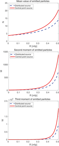
Some numerical examples in Fig. 2 show the first three factorial moments as a function of the radius of the sphere in optical units. For comparison with the case of the distributed source, each figure also shows the moments corresponding to the same sphere with a distributed source.

Fig. 2. First, second, and third moments of the number of neutrons emitted from a solid sphere for a distributed source (dashed lines, blue) and a central point source (solid lines, red) as functions of the outer radius $R$.

The input data of the spontaneous and induced fission multiplicities are given in Table I. These were taken from the material data of the Rocky Flats Shells (93% ²³⁵U and 7% ²³⁸U) and a ²⁵²Cf source.^5,6

TABLE I Input Parameters Used in the Calculations

	First Moment	Second Moment	Third Moment
Spontaneous fission (^252Cf)	${\nu }_{sf,1}=3.757$	${\nu }_{sf,2}=11.962$	${\nu }_{sf,3}=31.812$
Induced fission (93% ^235U + 7% ^238U at 2 MeV)	${\nu }_{r,1}=2.637$	${\nu }_{r,2}=5.623$	${\nu }_{r,3}=9.476$

The plots in Fig. 2 show that for the same size of the sphere, the moments corresponding to the source of the same strength and multiplicity located in the center are larger than those corresponding to the distributed source. This is expected since neutrons starting from the center of the sphere have a higher importance than those closer to the surface.

III.B. Point Source in a Cavity of a Shell

The treatment of an isotropic point source in the cavity requires some care because of the vacuum surrounding the source. In this vacuum the angular distribution of the neutrons is highly anisotropic, actually singular, since they are progressing radially out of the source. The isotropy of the source means that each neutron obeys an angular density $\delta (\mu -{\mu }_i)$ such that ${\mu }_i$ is distributed evenly between $[-1,1]$.

To handle such a source, one has to consider a more general description of the number distribution angular density of the source neutrons, as it was introduced in connection to the energy description of spallation neutrons.¹² In a one-speed description, still in spherical symmetry, one should consider the source distribution function $P_S(k,r,{\mu }_1,{\mu }_2,\dots {\mu }_k)$ such that

(37) $P_S(k,r,{\mu }_1,{\mu }_2,\dots {\mu }_k)r^{2}drd{\mu }_1\dots d{\mu }_k$(37)

is the probability that in one source event, there will be $k$ neutrons emitted around $r$ and ${\mu }_1,{\mu }_2,\dots {\mu }_k$. This general expression can be simplified if the number of neutrons generated is independent of the position and the directions are independent of both each other and the number of neutrons generated in the source event and the position. Further, if the angular distributions are uniform, then $P_S(k,r,{\mu }_1,{\mu }_2,\dots {\mu }_k)$ will be simplified to

(38) $P_S(k,r,{\mu }_1,{\mu }_2,\dots {\mu }_k)=p_s(k)p_r(r)f_{\mu }(\mu {)}^k,$(38)

where $f_{\mu }(\mu )$ is the uniform angular density.

Coming back now to the source in the cavity, since in the equation of the single particle–induced distributions only neutrons starting within the medium are considered, a practical way of treating the central source is to neglect the free flight of the neutrons and consider them only when they arrive at the surface of the cavity. Since all neutrons will arrive at the surface of the spherical cavity at the same radial distance $r_0$ in a direction perpendicular to the surface of the cavity, one will have

(39) $P_S(k,r,{\mu }_1,{\mu }_2,\dots {\mu }_k)=p_s(k)\frac{\delta (r-r_0)}{r^2}{\delta }^k(\mu -1).$(39)

Using this in the master equation leading to an expression for the generating function $G(z)$ will result in

(40) $G(z)=q_s\left[g(z|r_0,1)\right].$(40)

Similarly to the case of the point source in the solid sphere, Eq. (33(33) $G(z)=q_s\left[g(z|0)\right].$(33) ), the factorial moments obtained from Eq. (40)(40) $G(z)=q_s\left[g(z|r_0,1)\right].$(40) have the simple form

(41) $N={\nu }_{s,1}n(r_0,1),$(41)

(42) $M={\nu }_{s,2}{n}^2(r_0,1)+{\nu }_{s,1}m(r_0,1),$(42)

and

(43) $W={\nu }_{s,3}{n}^3(r_0,1)+3{\nu }_{s,2}n(r_0,1)m(r_0,1)+{\nu }_{s,1}w(r_0,1).$(43)

Apart from the fact that unlike in Eqs. (34)(34) $N={\nu }_{s,1}n(0),$(34) , (35)(35) $M={\nu }_{s,2}{n}^2(0)+{\nu }_{s,1}m(0),$(35) , and (36)(36) $W={\nu }_{s,3}{n}^3(0)+3{\nu }_{s,2}n(0)m(0)+{\nu }_{s,1}w(0).$(36) , it is the angular moments that occur and not the scalar ones, Eq. (41)(41) $N={\nu }_{s,1}n(r_0,1),$(41) , (42)(42) $M={\nu }_{s,2}{n}^2(r_0,1)+{\nu }_{s,1}m(r_0,1),$(42) , and (43)(43) $W={\nu }_{s,3}{n}^3(r_0,1)+3{\nu }_{s,2}n(r_0,1)m(r_0,1)+{\nu }_{s,1}w(r_0,1).$(43) have the same advantageous property that no integrals over the volume of the item need to be taken. Since the scalar single particle–induced moments can be calculated only through the calculation of their angular moments, the computational effort would be the same. However, it has to be kept in mind that both the generating function $g(z|r,\mu )$ and hence also its moments are not the same here as for the homogeneous medium. The moments in Eqs. (34)(34) $N={\nu }_{s,1}n(0),$(34) , (35)(35) $M={\nu }_{s,2}{n}^2(0)+{\nu }_{s,1}m(0),$(35) , and (36)(36) $W={\nu }_{s,3}{n}^3(0)+3{\nu }_{s,2}n(0)m(0)+{\nu }_{s,1}w(0).$(36) are calculated for the solid sphere, which has already been done in Ref. 3. The angular moments in Eqs. (41)(41) $N={\nu }_{s,1}n(r_0,1),$(41) , (42)(42) $M={\nu }_{s,2}{n}^2(r_0,1)+{\nu }_{s,1}m(r_0,1),$(42) , and (43)(43) $W={\nu }_{s,3}{n}^3(r_0,1)+3{\nu }_{s,2}n(r_0,1)m(r_0,1)+{\nu }_{s,1}w(r_0,1).$(43) , on the other hand, have to be calculated from the more involved equations such as Eqs. (20)(20) $\begin{array}{c}n(r,\mu )=\mathrm{\Delta }(\mu -{\mu }_{cr}(r))[e^{-\mathrm{\ell }(r,\mu )}+{\nu }_{r,1}{\int }_0^{\mathrm{\ell }(r,\mu )}ds{e}^{-s}n(r{ }^{\mathrm{\prime }}(s))]\\ +\mathrm{\Delta }({\mu }_{cr}(r)-\mu )[e^{-\mathrm{\ell }(r,\mu )+(s_2(r,\mu )-s_1(r,\mu ))}+{\nu }_{r,1}{\int }_0^{s_1(r,\mu )}ds{e}^{-s}n(r{ }^{\mathrm{\prime }}(s))\\ +{\nu }_{r,1}{e}^{[s_2(r,\mu )-s_1(r,\mu )]}{\int }_{s_2(r,\mu )}^{\mathrm{\ell }(r,\mu )}ds{e}^{-s}n(r{ }^{\mathrm{\prime }}(s))].\end{array}$(20) , (22)(22) $\begin{array}{c}m(r,\mu )=\mathrm{\Delta }(\mu -{\mu }_{cr}(r)){\int }_0^{\mathrm{\ell }(r,\mu )}ds{e}^{-s}\{{\nu }_{r,2}{n}^2(r{ }^{\mathrm{\prime }}(s))+{\nu }_{r,1}m(r{ }^{\mathrm{\prime }}(s))\}\\ +\mathrm{\Delta }({\mu }_{cr}(r)-\mu )[{\int }_0^{s_1(r,\mu )}ds{e}^{-s}\{{\nu }_{r,2}{n}^2(r{ }^{\mathrm{\prime }}(s))+{\nu }_{r,1}m(r{ }^{\mathrm{\prime }}(s))\}\\ +e^{(s_2(r,\mu )-s_1(r,\mu ))}{\int }_{s_2(r,\mu )}^{\mathrm{\ell }(r,\mu )}ds{e}^{-s}\{{\nu }_{r,2}{n}^2(r{ }^{\mathrm{\prime }}(s))+{\nu }_{r,1}m(r{ }^{\mathrm{\prime }}(s))]\}\end{array}$(22) and (25)(25) $\begin{array}{c}w(r,\mu )=\mathrm{\Delta }(\mu -{\mu }_{cr}(r)){\int }_0^{\mathrm{\ell }(r,\mu )}ds{e}^{-s}\left\{{\nu }_{r,3}{n}^3(r{ }^{\mathrm{\prime }}(s))+3{\nu }_{r,2}n(r{ }^{\mathrm{\prime }}(s))m(r{ }^{\mathrm{\prime }}(s))+{\nu }_{r,1}w(r{ }^{\mathrm{\prime }}(s))\right\}\\ +\mathrm{\Delta }({\mu }_{cr}(r)-\mu )\left[{\int }_0^{s_1(r,\mu )}ds{e}^{-s}\left\{{\nu }_{r,3}{n}^3(r{ }^{\mathrm{\prime }}(s))+3{\nu }_{r,2}n(r{ }^{\mathrm{\prime }}(s))m(r{ }^{\mathrm{\prime }}(s))+{\nu }_{r,1}w(r{ }^{\mathrm{\prime }}(s))\right\}\right.\\ \left.+e^{(s_2(r,\mu )-s_1(r,\mu ))}{\int }_{s_2(r,\mu )}^{\mathrm{\ell }(r,\mu )}ds{e}^{-s}\left\{{\nu }_{r,3}{n}^3(r{ }^{\mathrm{\prime }}(s))+3{\nu }_{r,2}n(r{ }^{\mathrm{\prime }}(s))m(r{ }^{\mathrm{\prime }}(s))+{\nu }_{r,1}w(r{ }^{\mathrm{\prime }}(s))\right\}\right]\end{array}$(25) , or from the scalar moment Eqs. (21)(21) $\begin{array}{c}n(r)=n_0(r)+\frac{{\nu }_{r,1}}{2}\left[{\int }_{-1}^{{\mu }_{cr}}d\mu \left\{{\int }_0^{s_1(r,\mu )}ds{e}^{-s}n(r{ }^{\mathrm{\prime }}(s))\right.\right.\\ +\left.\left.e^{[s_2(r,\mu )-s_1(r,\mu )]}{\int }_{s_2(r,\mu )}^{\mathrm{\ell }(r,\mu )}ds{e}^{-s}n(r{ }^{\mathrm{\prime }}(s))\right\}+{\int }_{{\mu }_{cr}}^{1}d\mu {\int }_0^{\mathrm{\ell }(r,\mu )}ds{e}^{-s}n(r{ }^{\mathrm{\prime }}(s))\right],\end{array}$(21) , (23)(23) $\begin{array}{c}m(r)=m_0(r)+\frac{{\nu }_{r,1}}{2}\left[{\int }_{-1}^{{\mu }_{cr}}d\mu \left\{{\int }_0^{s_1(r,\mu )}ds{e}^{-s}m(r{ }^{\mathrm{\prime }}(s))\right.\right.\\ +\left.\left.e^{[s_2(r,\mu )-s_1(r,\mu )]}{\int }_{s_2(r,\mu )}^{\mathrm{\ell }(r,\mu )}ds{e}^{-s}m(r{ }^{\mathrm{\prime }}(s))\right\}+{\int }_{{\mu }_{cr}}^{1}d\mu {\int }_0^{\mathrm{\ell }(r,\mu )}ds{e}^{-s}m(r{ }^{\mathrm{\prime }}(s))\right]\end{array}$(23) , and (26)(26) $\begin{array}{c}w(r)=w_0(r)+\frac{{\nu }_{r,1}}{2}\left[{\int }_{-1}^{{\mu }_{cr}}d\mu \left\{{\int }_0^{s_1(r,\mu )}ds{e}^{-s}w(r{ }^{\mathrm{\prime }}(s))\right.\right.+\left.\left.e^{[s_2(r,\mu )-s_1(r,\mu )]}{\int }_{s_2(r,\mu )}^{\mathrm{\ell }(r,\mu )}ds{e}^{-s}w(r{ }^{\mathrm{\prime }}(s))\right\}+{\int }_{{\mu }_{cr}}^{1}d\mu {\int }_0^{\mathrm{\ell }(r,\mu )}ds{e}^{-s}w(r{ }^{\mathrm{\prime }}(s))\right]\end{array}$(26) , and by converting them to the corresponding angular moments by relations of the Eq. (28)(28) $n(r,\mu =1)=e^{-(R-r)}+{\nu }_{r,1}{\int }_0^{(R-r)}ds{e}^{-s}n(r+s)$(28) type.

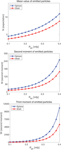
Calculations for shells have been performed for cases with various inner and outer shell radii, with the same material data as in Table I. One set of results with a fixed inner radius and varying outer radii is shown in Fig. 3. It is seen that as it could be expected, all moments for the sphere with an equal outer radius are higher than for the shell. This is naturally due to the lower internal multiplication (smaller mass) of the shell, due to the central cavity.

Fig. 3. First, second, and third moments of the number of neutrons emitted from a solid sphere (blue lines, marked with circles) and a shell with an inner radius $r_0=0.1$ mean free path (red lines, marked with triangles), both with a central source. $R_{eff}$ is the outer radius in optical units for both cases.

It is worth adding that the main incentive of the work described so far is not to show that a central source leads to higher internal multiplication than an equivalent distributed one or that a solid sphere leads to higher internal multiplication than a shell with the same central point source. These results are trivial and could be predicted without calculations, and the fact that they could be reproduced just makes the results, and hence the formalism, plausible. The main purpose was to elaborate a formalism that makes it possible to obtain quantitative results such that they can be used for multiplicity counting for items with a shell geometry and a central source and that can also be compared against the measurements, as will be done in the next section.

IV. INCLUSION OF SCATTERING

Results of calculations based on the formalism developed above for shells were compared with the preliminary results of the measurements made on the Rocky Flats Shells during the MUSIC campaign.^5–8 The building blocks of these shells are highly enriched hemispheres of metallic uranium (93% ²³⁵U and 7% ²³⁸U), which can be nested into each other to form solid spheres or thick shells of various sizes from pairs of identical hemispheres. Measurements were analyzed for four configurations of the Rocky Flats Shells measured by the Neutron Multiplicity Array Detector (NoMAD), 15 tubes embedded within a high-density polyethylene (HDPE) matrix.¹³ Evaluation of the singles, doubles, and triples (S, D, and T) rates on shells with the same inner radius and four different outer radii, using a ²⁵²Cf source in the central cavity were completed.¹⁴ The factorial moments of the source-induced emission were derived from the S, D, and T rates, using the source intensity and the detector efficiency of the detectors used in the experiment.

The calculations were first performed for the same physical sizes as the experiments, assuming induced fission as the only neutron reaction, similarly to the procedure used in the point model. The measurements were made with a compilation of Rocky Flats Shell sets with an inner radius of 2.0126 cm and outer radii of $R=$ 5.6692, 6.6696, 7.3296, and 8.0027 cm, respectively. The quantitative results obtained from the formulas developed in the preceding sections deviated from the measured ones; all calculated moments were systematically lower than the measured ones (shown later in Fig. 5). This indicated that the calculations underestimated the internal multiplication.

One might assume some reasons for this difference between the measurements and the calculations. One reason could be possible uncertainties in the extraction of the factorial moments from the measured S, D, and T rates in the measurements. Also, there is the further circumstance that the calculations were made for solid hemispheres whereas in the Rocky Flats Shells, there are gaps between the layers of the nested hemispheres.^7,8

Hence, a somewhat more straightforward and unambiguous way of checking the fidelity of the calculated results was chosen. It is the calculation of the critical radii of pure solid spheres of ²³⁵U and ²³⁹Pu for which well-known data are available in the literature. Although in principle this only proves the correctness of the calculation of the first moment, it is still a good indicator of the fidelity of the model.

For the critical radii of a solid sphere of pure ²³⁵U and pure ²³⁹Pu, the calculations yield the following values, respectively:

(44) $R_{crit}^{\mathrm{U}235}=10.46\mathrm{c}\mathrm{m};(\mathrm{t}\mathrm{r}\mathrm{u}\mathrm{e}\mathrm{v}\mathrm{a}\mathrm{l}\mathrm{u}\mathrm{e}:8.5\mathrm{c}\mathrm{m})$(44)

and

(45) $R_{crit}^{\mathrm{P}\mathrm{u}239}=5.33\mathrm{c}\mathrm{m};(\mathrm{t}\mathrm{r}\mathrm{u}\mathrm{e}\mathrm{v}\mathrm{a}\mathrm{l}\mathrm{u}\mathrm{e}:4.97\mathrm{c}\mathrm{m}).$(45)

For the Rocky Flats Shells, the critical size of a solid sphere is about 8.83 cm, but this is partly because the shells consist of 93% ²³⁵U and 7% ²³⁸U and partly because of the gap between the shell layers.^7,8

The above differences for the factorial moments and the critical sizes both point to the same direction, namely, that the model developed on the same assumptions as the point model, which regards the reactions that the neutrons undergo (only fission), underestimates the internal multiplication (or overestimates leakage). Since the boundary conditions are properly accounted for in the model, a rather natural first guess for the reason for this deviation is that other processes, and primarily scattering, are not taken into account. For instance, at the average energy of the source neutrons, taken in the present one-speed model as 2 MeV (the same energy value usually used in the point model), the macroscopic elastic scattering cross section for ²³⁵U is about three times larger than the fission cross section. Scattering within the item has a similar effect as a reflector surrounding the core; i.e., it increases the internal multiplication; hence, its effect has to be taken into account.

The reason why in the point model, scattering is not explicitly accounted for is that in the point model equations, in which phase-space coordinates such as position and direction of traveling do not appear, scattering is a “non-event,” consisting of a reaction where one neutron before the collision produces one outgoing neutron. This is a situation similar to the traditional point theory of the Feynman-alpha and Rossi-alpha methods, where only fission and absorption are accounted for. In the point model of multiplicity counting, the influence of the position and velocity direction on leakage is condensed into the first collision probability (embedded into the leakage multiplication), which is one of the unknowns of the process.

Therefore, it appears advisable to try to include elastic scattering as a first step into the generalization of the model. As it turns out, accounting for elastic scattering in the model is relatively straightforward. Since elastic scattering of neutrons on heavy nuclei can be assumed to be isotropic to a very good approximation and since energy loss of the neutrons can be neglected, the hitherto used one-speed transport theory with isotropic scattering can be kept. In this model, elastic scattering is equivalent to a fission event with one fission neutron generated. One can include such a process in the model by switching to using the number distribution of neutrons per reaction as a weighted average of the number distribution of induced fission and the singular distribution (a Kronecker delta) of the scattering and correspondingly using the total cross section for the unit of the mean free path. The procedure is completely analogous to how the joint number distribution of source neutrons is calculated as a weighted average of the distributions of spontaneous fission neutrons and that of the $(\alpha ,n)$ neutrons or how the number distribution of the number of neutrons from a reaction is calculated from the number distribution of induced fission and absorption in Ref. 9. We mention here in passing that likewise, absorption can be included in the present model as a fission event with zero generated neutrons. However, because of the negligibly small absorption cross section, this possibility is not considered here.

In formulas, we introduce the total cross section as

(46) ${\mathrm{\Sigma }}_T={\mathrm{\Sigma }}_f+{\mathrm{\Sigma }}_{el}$(46)

and the number distribution of neutrons from a reaction (also called secondaries) as the weighted sum

(47) $p_r(k)=\frac{{\mathrm{\Sigma }}_f}{{\mathrm{\Sigma }}_T}{f}_k+\frac{{\mathrm{\Sigma }}_{el}}{{\mathrm{\Sigma }}_T}{\delta }_{k,1}\equiv {\alpha }_s{f}_k+{\beta }_s{\delta }_{k,1}.$(47)

Here, as before, $f_k$ stands for the number distribution of induced fission neutrons; ${\delta }_{k,1}$ is a Kronecker symbol; and ${\alpha }_s$ and ${\beta }_s$ are the fractional contributions of fission and elastic scattering cross sections to the total cross section, respectively. Then, the size of the item in optical units is determined by ${\mathrm{\Sigma }}_T$ whereas the number distribution of the neutrons per reaction is given by Eq. (47)(47) $p_r(k)=\frac{{\mathrm{\Sigma }}_f}{{\mathrm{\Sigma }}_T}{f}_k+\frac{{\mathrm{\Sigma }}_{el}}{{\mathrm{\Sigma }}_T}{\delta }_{k,1}\equiv {\alpha }_s{f}_k+{\beta }_s{\delta }_{k,1}.$(47) . As mentioned above, Eqs. (46)(46) ${\mathrm{\Sigma }}_T={\mathrm{\Sigma }}_f+{\mathrm{\Sigma }}_{el}$(46) and (47(47) $p_r(k)=\frac{{\mathrm{\Sigma }}_f}{{\mathrm{\Sigma }}_T}{f}_k+\frac{{\mathrm{\Sigma }}_{el}}{{\mathrm{\Sigma }}_T}{\delta }_{k,1}\equiv {\alpha }_s{f}_k+{\beta }_s{\delta }_{k,1}.$(47) ) could easily be extended to include absorption, containing a ${\delta }_{n,0}$ term. However, since absorption is low at these neutron energies in the given nuclei, this inclusion is not considered here.

The above means that the factorial moments ${\nu }_{r,i},i=1,2,3$ of the distribution $p_r(k)$ will enter the moment equations. From Eq. (47(47) $p_r(k)=\frac{{\mathrm{\Sigma }}_f}{{\mathrm{\Sigma }}_T}{f}_k+\frac{{\mathrm{\Sigma }}_{el}}{{\mathrm{\Sigma }}_T}{\delta }_{k,1}\equiv {\alpha }_s{f}_k+{\beta }_s{\delta }_{k,1}.$(47) ), these are readily obtained as

(48) ${\nu }_{r,i}={\alpha }_s{\nu }_{f,i}+{\beta }_s{\delta }_{i,1}.$(48)

To see the effect of scattering on the quantitative values of the factorial moments, first, the following conceptual calculations were performed. We started with a solid sphere with no scattering—only fission included. To calculate the size of the sphere in optical units (which is employed in the formulas), the ²³⁵U fission cross section at 2 MeV, ${\mathrm{\Sigma }}_f$ = 0.0621125 cm^–1, was used. Thereafter, we added scattering such that the scattering cross section became 25%, 50%, and 75% of the total cross section. The case of only fission thus corresponds to ${\beta }_s=0$, and the realistic case for ²³⁵U is close to ${\beta }_s=\mathrm{0.75.}$

The effect of scattering is illustrated in Fig. 4, showing the factorial moments as functions of the physical sphere radius for different values of the relative weight ${\beta }_s$ of the elastic scattering cross section to the total cross section. Calculations were made for a sphere radius up to 7 cm. In the plots, the physical size of the sphere was used as the independent variable because when scattering is included, the total cross section and hence also the optical path length change. Thus, although the physical size of the sphere does not change, its size in terms of the mean free path changes for different extents of scattering included. For a fair comparison, we need to use the physical size as the independent variable.

Fig. 4. The first three factorial moments as functions of the radius of a pure ²³⁵U sphere, with varying degrees ${\beta }_s$ of elastic scattering being included. Left column: full range ($R$ between 0 and 7 cm); right column: half range ($R$ between 0 and 3.5 cm).

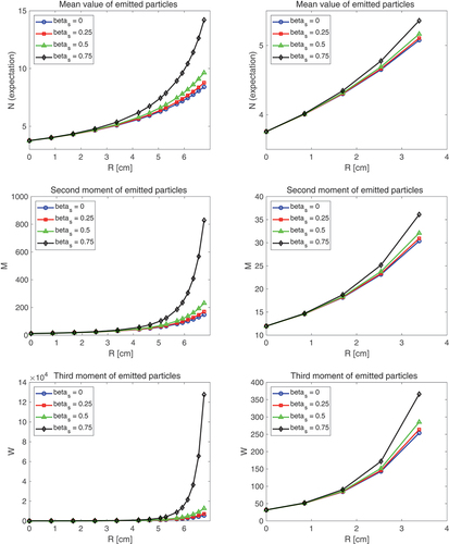
In Fig. 4, the left column shows the results for the whole range ($R$ between 0 and 7 cm) whereas the right column does it for the half range $0<R<3.5$ cm since in the full-range plot, the differences in the various moments for small $R$ values are not visible. The figure shows that inclusion of scattering increases the factorial moments; the higher the contribution from scattering is, the higher the moments become. Scattering processes close to the boundary might both increase leakage and act as a reflector whereas scattering farther away from the boundary might mostly act as a reflector. It appears that the reflector effect dominates over the outscatter processes, and increasingly so for increasing sphere radii.

It is also seen that even with a relative contribution of scattering with ${\beta }_s=0.75$, for small sizes, up to about $R=2$ cm, the effect of scattering is minor. However, the deviation between the cases of no scattering and scattering increases fast with increasing size of the system; moreover, the relative deviation increases also with the moment order. Approaching the critical size of the case with scattering (which is smaller than with only fission), the deviations diverge.

It is now interesting to check the improvement in the fidelity of the model both by calculating the critical sizes of pure ²³⁵U and ²³⁹Pu spheres and by comparing the factorial moments obtained experimentally for the Rocky Flats Shells. With regard to critical sizes, making calculations with the inclusion of scattering and using the elastic scattering cross sections of ²³⁵U and ²³⁹Pu at 2 MeV yield the results

(49) $R_{crit}^{\mathrm{U}235}=8.043\mathrm{c}\mathrm{m};(\mathrm{t}\mathrm{r}\mathrm{u}\mathrm{e}\mathrm{v}\mathrm{a}\mathrm{l}\mathrm{u}\mathrm{e}:8.5\mathrm{c}\mathrm{m})$(49)

and

(50) $R_{crit}^{\mathrm{P}\mathrm{u}239}=4.527\mathrm{c}\mathrm{m};(\mathrm{t}\mathrm{r}\mathrm{u}\mathrm{e}\mathrm{v}\mathrm{a}\mathrm{l}\mathrm{u}\mathrm{e}:4.97\mathrm{c}\mathrm{m}).$(50)

A comparison with the case when only fission is accounted for, Eqs. (44)(44) $R_{crit}^{\mathrm{U}235}=10.46\mathrm{c}\mathrm{m};(\mathrm{t}\mathrm{r}\mathrm{u}\mathrm{e}\mathrm{v}\mathrm{a}\mathrm{l}\mathrm{u}\mathrm{e}:8.5\mathrm{c}\mathrm{m})$(44) and (45(45) $R_{crit}^{\mathrm{P}\mathrm{u}239}=5.33\mathrm{c}\mathrm{m};(\mathrm{t}\mathrm{r}\mathrm{u}\mathrm{e}\mathrm{v}\mathrm{a}\mathrm{l}\mathrm{u}\mathrm{e}:4.97\mathrm{c}\mathrm{m}).$(45) ), shows that the accuracy of calculated critical radius is now significantly better, especially for ²³⁵U. It is also seen that accounting for elastic scattering, the model now slightly overestimates the internal multiplication. The same tendency is seen also on the calculated factorial moments. These are now larger than without scattering, but they are also larger than the measured ones, as is seen in Fig. 5, showing both the preliminary experimental results and the calculated results with and without scattering (${\beta }_s=0.753$ and 0, respectively).

Fig. 5. Comparison of measured and calculated first, second, and third moments of the number of neutrons emitted from the Rocky Flats Shells for four different outer radii and with an inner radius of 2.0126 cm.

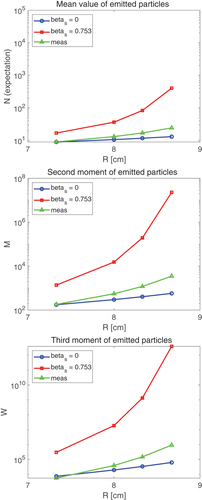
Figure 5 also shows that unlike for the critical radii, the deviation between the measured and the calculated values is larger when scattering is included than without scattering. This indicates that accounting for elastic scattering, even if it improves the fidelity of the model, is still not sufficient for good agreement with measurements. The remaining possible reason for the difference between the calculated and the measured values can be sought in the neglect of inelastic scattering. In an inelastic scattering event, the neutron energy decreases significantly. At the lower energy of the inelastically scattered neutrons, both the cross sections and the fission neutron multiplicities are different, which may have a nonnegligible impact on the internal multiplication and transport process.

The present one-speed transport theory model used so far is obviously not suitable to treat inelastic scattering. In order to extend the model to be able to handle inelastic scattering properly, one should introduce energy dependence and anisotropic scattering. Formally, both of these aspects can easily be included in the model, as will be shown in coming publications.¹⁵ However, the main stumbling block will be the fact that the cross sections, the fission neutron multiplicities, and the scattering function will become energy dependent. Even if it is possible to restrict the relevant energy range to above the resonance region, this will require the handling of extensive data tables and excessive running times.

Although the above path will be explored in future work, for the time being, we note that there exists a simpler, even if empirical, fix to account for inelastic scattering approximately in a one-speed model. In Ref. 16, it is suggested that in view of the fact that the average energy of once inelastically scattered neutrons is about 1 MeV, one gets a better estimate of the critical mass if the relevant cross sections and multiplicities are taken at 1 MeV.

We tested this suggestion first for the critical masses predicted by the model. The multiplicities for induced fission of ²³⁵U and ²³⁹Pu at 1 MeV are available in Ref. 17. Taking into account fission and elastic scattering with cross sections at 1 MeV, the following results are obtained:

(51) $R_{crit}^{\mathrm{U}235}=8.623\mathrm{c}\mathrm{m};(\mathrm{t}\mathrm{r}\mathrm{u}\mathrm{e}\mathrm{v}\mathrm{a}\mathrm{l}\mathrm{u}\mathrm{e}:8.5\mathrm{c}\mathrm{m})$(51)

and

(52) $R_{crit}^{\mathrm{P}\mathrm{u}239}=5.295\mathrm{c}\mathrm{m};(\mathrm{t}\mathrm{r}\mathrm{u}\mathrm{e}\mathrm{v}\mathrm{a}\mathrm{l}\mathrm{u}\mathrm{e}:4.97\mathrm{c}\mathrm{m}).$(52)

Compared with Eqs. (49)(49) $R_{crit}^{\mathrm{U}235}=8.043\mathrm{c}\mathrm{m};(\mathrm{t}\mathrm{r}\mathrm{u}\mathrm{e}\mathrm{v}\mathrm{a}\mathrm{l}\mathrm{u}\mathrm{e}:8.5\mathrm{c}\mathrm{m})$(49) and (50(50) $R_{crit}^{\mathrm{P}\mathrm{u}239}=4.527\mathrm{c}\mathrm{m};(\mathrm{t}\mathrm{r}\mathrm{u}\mathrm{e}\mathrm{v}\mathrm{a}\mathrm{l}\mathrm{u}\mathrm{e}:4.97\mathrm{c}\mathrm{m}).$(50) ), an improvement is seen in the prediction of the critical radius, especially for ²³⁵U. It is also seen that with this empirical correction, the model again underestimates the internal multiplication (overestimates the critical radius).

A more interesting question is how the use of the cross sections and multiplicities at 1-MeV neutron energy would affect the calculated values of the factorial moments, which by using data at 2 MeV overestimate the measured ones significantly. Here, too, one might expect a larger effect of using data at 1 MeV since the fission cross section–induced fission neutron multiplicities are all lower than at 2 MeV, especially for ²³⁸U content.

The factorial moments of the number of neutrons emitted per one source event (²⁵²Cf spontaneous fission) from an item with the geometrical and material properties of the Rocky Flats Shells were calculated with the cross sections and multiplicities of ²³⁵U and ²³⁸U taken at 1 MeV. The fission and elastic scattering cross sections of the mixture of the two isotopes were calculated in the standard way, that is,¹⁸

(53) ${\mathrm{\Sigma }}_i^x={\sigma }_i^x{w}_i\rho \frac{N_{Avo}}{M_i}$(53)

with $x$ representing the reaction type and $i$ the nuclide index in question (235 or 238), $w_i$ being the weight fraction of the corresponding isotope, and $\rho =$ 18.664 g/cm³ being the density of the compound. The fission number distribution $f_k$ of the compound was calculated as

(54) $f_k=\frac{{\mathrm{\Sigma }}_f^{235}}{{\mathrm{\Sigma }}_f}{f}_k^{235}+\frac{{\mathrm{\Sigma }}_f^{238}}{{\mathrm{\Sigma }}_f}{f}_k^{238}$(54)

with ${\mathrm{\Sigma }}_f={\mathrm{\Sigma }}_f^{235}+{\mathrm{\Sigma }}_f^{238}$. The number distributions $f_k^{255}$ and $f_k^{238}(k)$ were taken from Verbeke et al.¹⁷ With these, similarly to Eq. (47(47) $p_r(k)=\frac{{\mathrm{\Sigma }}_f}{{\mathrm{\Sigma }}_T}{f}_k+\frac{{\mathrm{\Sigma }}_{el}}{{\mathrm{\Sigma }}_T}{\delta }_{k,1}\equiv {\alpha }_s{f}_k+{\beta }_s{\delta }_{k,1}.$(47) ), the number distribution $p_r(k)$ of the secondaries in a reaction when both fission and scattering are accounted for is obtained as

(55) $p_r(k)=\frac{{\mathrm{\Sigma }}_f}{{\mathrm{\Sigma }}_T}{f}_k+\frac{{\mathrm{\Sigma }}_{el}}{{\mathrm{\Sigma }}_T}{\delta }_{k,1}\equiv {\alpha }_s{f}_k+{\beta }_s{\delta }_{k,1}.$(55)

Here, ${\mathrm{\Sigma }}_{el}={\mathrm{\Sigma }}_{el}^{235}+{\mathrm{\Sigma }}_{el}^{238}$ and ${\mathrm{\Sigma }}_T={\mathrm{\Sigma }}_f+{\mathrm{\Sigma }}_{el}$. Naturally, the formal relationships between the factorial moments of pure fission and those of fission plus scattering are the same as in Eq. (48(48) ${\nu }_{r,i}={\alpha }_s{\nu }_{f,i}+{\beta }_s{\delta }_{i,1}.$(48) ); that is,

(56) ${\nu }_{r,i}={\alpha }_s{\nu }_{f,i}+{\beta }_s{\delta }_{i,1},$(56)

where $i$ is the moment order.

The numerical values of the cross sections of the compound, used in the calculations, are given in Table II, and the factorial moments of the number distribution of fission neutrons and those of the secondaries with elastic scattering included are given in Table III. The factorial moments of the source emission neutrons are the same as given in the first row of Table I.

TABLE II Macroscopic Cross Sections of the Rocky Flats Shells at 1 MeV*

	$93\mathrm{\%}$ ^235U	$7\mathrm{\%}$ ^238U	93% ^235U + 7% ^238U
${\mathrm{\Sigma }}_f$	${\mathrm{\Sigma }}_f^{235}=0.05351$	${\mathrm{\Sigma }}_f^{238}$=0.0000482	${\mathrm{\Sigma }}_f=0.05355$
${\mathrm{\Sigma }}_{el}$	${\mathrm{\Sigma }}_{el}^{235}=0.17225$	${\mathrm{\Sigma }}_{el}^{238}=0.014068$	${\mathrm{\Sigma }}_{el}=0.18632$
${\mathrm{\Sigma }}_T$			${\mathrm{\Sigma }}_T$ = 0.23988

*In units of cm⁻¹.

TABLE III Factorial Moments of the Rocky Flats Shells at 1 MeV

	First Moment	Second Moment	Third Moment
Induced fission	${\nu }_{f,1}=2.52359$	${\nu }_{f,2}=5.10119$	${\nu }_{f,3}=8.00135$
Fission plus elastic scattering	${\nu }_{r,1}=1.34015$	${\nu }_{r,2}=1.13887$	${\nu }_{r,3}=1.78635$

Figure 6 compares the preliminary results of the measurements and the calculated values, with and without scattering. The figure shows that with accounting for elastic scattering and assuming an average neutron energy of 1 MeV, the calculated values agree with the measured ones remarkably well, especially for the first moment. With increasing moment order, the agreement slightly worsens.

Fig. 6. Comparison of measured and calculated first, second, and third moments of the number of neutrons emitted from the Rocky Flats Shells for four different outer radii and with an inner radius of 2.0126 cm. In the calculated values, the material properties correspond to those of the isotopic composition of the Rocky Flats Shells at a neutron energy of 1 MeV.

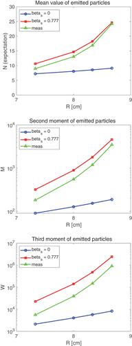
It might sound contradictory that one accounts for the effect of inelastic scattering by merely changing the average energy of neutrons in the system but without accounting for the cross section of inelastic scattering. However, it has to be kept in mind that this is only a phenomenological, approximative treatment. Neglecting the actual inelastic scattering events is compensated by the fact that one takes 1 MeV as the average energy of neutrons in the system whereas in reality, 1 MeV is only the average energy of the neutrons after one inelastic collision, which is less than half of all neutrons generated in a single chain.

In summary, accounting for elastic scattering properly in the formalism and modifying the model empirically to account for inelastic scattering in an approximate manner, we found good agreement between calculations and measurements. This is very promising from the point of view that by accounting for inelastic scattering properly in an energy-dependent treatment with anisotropic scattering, even better agreement will be found. Work is already underway in this direction.

V. CONCLUSIONS

With the extension of the one-speed transport theory model, developed in our earlier work, to shells with a central cavity and central point source with inclusion of elastic scattering, and accounting for the effect of inelastic scattering in an empirical way, rather good agreement was found between the calculated values of the factorial moments with the preliminary results of the measurements made on the Rocky Flats Shells.^5,6 This suggests that it is worth pursuing the extension of the model to include energy dependence and anisotropic scattering such that the effect of inelastic scattering can be accounted for in an exact way. The conceptual extension of the model is rather straightforward¹⁵; on the practical side, the complexity of the calculations will increase significantly, and the computational burden might prove prohibitive.

It is also seen that in the transport model developed by us, most aspects of the physical process, such as the various reaction types, presence of a mixture of different nuclides, arrangement geometry, etc., can be taken into account, which the point model cannot do. This means that for a given item, the factorial moments can be predicted with a much higher accuracy than the point model would do. The question is, however, how much this enhanced capability can be utilized for the very purpose of material identification, i.e., to solve the inverse task of determining the fissile mass of the item from the measured S, D, and T rates. Namely, the enhanced capabilities of the model come with the price that it contains a large number of parameters, all of which in principle would need to be determined (and/or several be known in advance) in an unfolding procedure in order to extract the only important parameter, the source fission rate. This would be even more complicated if ($\alpha ,n$) reactions were included. Despite all the approximations that its application incurs, the advantages of the point model, as is the case with all lumped parameter models such as the Feynman-alpha and Rossi-alpha methods, are that it contains a very small set of parameters, which can be unfolded by an analytical inversion of the simple algebraic formulas, and that the model is robust, i.e., not very sensitive to fine geometrical and material details (within certain limits).

For the space-dependent model, an analytical unfolding procedure is obviously not possible since even the direct task, i.e., the calculation of the factorial moments, is only possible numerically. However, an unfolding is achievable based on machine learning methods (artificial neural networks). It is here that the larger resolution of the details in the space-dependent model may come to an advantage. Namely, since the properties of both the fissile and the fissionable material are included in the calculation of the factorial moments, it might be possible to determine the amount of fissile mass contained in the sample, which is impossible using the point model, which can determine only the fissionable content of the sample, that usually plays the role of the source. Examining the potentials of the space-dependent model for determining sample parameters is the most important next step that will need to be explored.

Acknowledgments

The authors are indebted to Prof. Senada Avdic (University of Tuzla) for interesting discussions and for supplying nuclear data for the calculations. The experiments in this work would not be possible without the contributions of the scientists of the Los Alamos National Laboratory (LANL) Advanced Nuclear Technology (NEN-2) National Criticality Experiments Research Center Team and in particular the support, coordination, and direction from Jesson Hutchinson and Dr. Geordie McKenzie and the measurements and analysis completed by Alexander McSpaden. Dr. Michael Hua and Prof. Sara Pozzi were also crucial in supporting, coordinating, and directing the University of Michigan’s participation in the MUSIC campaign and advising analysis of the measured experimental data. The computations presented in this paper were enabled by resources provided by the Swedish National Infrastructure for Computing (SNIC) at the Chalmers Centre for Computational Science and Engineering (C3SE), partially funded by the Swedish Research Council through grant agreement number 2018-05973. Mikael Öhman at C3SE is acknowledged for assistance concerning technical and implementational aspects in making the code run on the SNIC resources.

Disclosure Statement

No potential conflict of interest was reported by the author(s).

Additional information

Funding

This work received financial support from the Adlerbert Research Foundation, through the Royal Society of Arts and Sciences in Gothenburg. This work is supported by the Department of Energy (DOE) Nuclear Criticality Safety Program, funded and managed by the National Nuclear Security Administration (NNSA), the Consortium for Monitoring, Technology, and Verification under DOE NNSA award number DE-NA0003920, the DOE through the Los Alamos National Laboratory (LANL) operated by Triad National Security, LLC, for the NNSA under Contract No. 89233218CNA000001, and the DOE LDRD program at LANL.

Notes

^a This approach, also called the regeneration point technique, was originally developed in connection with cosmic electron-photon showers.¹¹

References

- K. BÖHNEL, “The Effect of Multiplication on the Quantitative Determination of Spontaneously Fissioning Isotopes by Neutron Correlation Analysis,” Nucl. Sci. Eng., 90, 75 (1985); https://doi.org/10.13182/NSE85-2.
- I. PÁZSIT, L. PÁL, and A. ENQVIST, “Extension of the Böhnel Model of Multiplicity Counting to Include Space- and Angular Dependence,” Proc. 60th INMM Annual Mtg., Palm Desert, California, July 14–18, 2019, Institute of Nuclear Materials Management (2019).
- I. PÁZSIT and L. PÁL, “Multiplicity Theory Beyond the Point Model,” Ann. Nucl. Energy, 154, 108119 (2021); https://doi.org/10.1016/j.anucene.2020.108119.
- I. PÁZSIT and V. DYKIN, “Transport Calculations of the Multiplicity Moments for Cylinders,” Nucl. Sci. Eng., 196, 235 (2022); https://doi.org/10.1080/00295639.2021.1973178.
- F. DARBY et al., “Examination of New Theory for Neutron Multiplicity Counting of Non-Point-Like Sources of Special Nuclear Material,” Proc. INMM & ESARDA Joint Virtual Annual Mtg., August 23—September 1, 2021, Institute of Nuclear Materials Management and European Safeguards Research and Development Association (2021).
- F. DARBY et al., “Comparison of Neutron-Multiplicity-Counting Estimates with Trans-Stilbene, EJ-309, and He-3 Detection Systems,” Trans. Am. Nucl. Soc., 125, 602 (2021).
- A. MCSPADEN et al., “MUSIC: A Critical and Subcritical Experiment Measuring Highly Enriched Uranium Shells,” Proc. 11th Int. Conf. Nuclear Criticality Safety (ICNC), Paris, France, September 15–20, 2019.
- A. T. MCSPADEN, G. E. MCKENZIE, and R. G. SANCHEZ, “Progress Update on the MUSIC Critical Benchmark,” LA-UR-22-26184, Los Alamos National Laboratory (2022); https://www.osti.gov/biblio/1897647.
- I. PÁZSIT and L. PÁL, Neutron Fluctuations: A Treatise on the Physics of Branching Processes, Elsevier (2008).
- N. ENSSLIN et al., “Application Guide to Neutron Multiplicity Counting,” LA-13422-M, Los Alamos National Laboratory (1998).
- L. JÁNOSSY, “Note on the Fluctuation Problem of Cascades,” Proc. Phys. Soc., 63, 241 (1950); https://doi.org/10.1088/0370-1298/63/3/307.
- I. PÁZSIT, “The Backward Theory of Stochastic Particle Transport with Multiple Emission Sources,” Phys. Scr., 59, 5, 344 (1999); https://iopscience.iop.org/article/10.1238/Physica.Regular.059a00344/meta.
- A. MCSPADEN et al., “Preliminary NoMAD Results of the MUSiC Experiment,” Trans. Am. Nucl. Soc., 125, 598 (2021); https://www.osti.gov/biblio/1899323.
- W. HAGE and D. M. CIFARELLI, “On the Factorial Moments of the Neutron Multiplicity Distribution of Fission Cascades,” Nucl. Instrum. Methods Phys. Res. Sect. A, 236, 165 (1985); https://doi.org/10.1016/0168-9002(85)90142-1.
- I. PÁZSIT, V. DYKIN, and S. AVDIC, “Transport Calculation of the Multiplicity Moments with Energy Dependence and Anisotropic Scattering,” Proc. Int. Conf. Mathematics and Computational Methods Applied to Nuclear Science and Engineering (M&C 2023), Niagara Falls, Ontario, Canada, April 13–17, 2023, American Nuclear Society (2023).
- C. SUBLETTE, “Nuclear Weapons Frequently Asked Questions,” Sec. 4.1, (2019); http://nuclearweaponarchive.org/.
- J. M. VERBEKE, C. HAGMAN, and D. WRIGHT, “Simulation of Neutron and Gamma Ray Emission from Fission and Photofission,” UCRL-AR-228518, Lawrence Livermore National Laboratory (2010).
- R. J. J. STAMMLER and M. J. ABBATE, Methods of Steady State Reactor Physics in Nuclear Design, Academic Press, London (1983).