Application of the Gauss-Seidel Method to the Chebyshev Rational Approximation Method for Solving Nuclear Fuel Depletion Systems

Abstract

The Chebyshev Rational Approximation Method (CRAM) has become one of the dominant methods for solving the Bateman equations for nuclear fuel depletion analysis. Since its introduction over a decade ago, several improvements have been made to CRAM improving its accuracy and reducing its run time. We analyzed its run time using two previously published methods for solving the CRAM system of equations, direct matrix inversion (DMI) and sparse Gaussian elimination (SGE), for depletion systems of varying numbers of nuclides to see how the two methods perform relative to one another. In addition to these two methods, we introduced the Gauss-Seidel (GS) method for solving the CRAM system of equations and compared its performance relative to DMI and SGE for depletion systems with varying numbers of nuclides. We demonstrated that for practical purposes, GS is faster than SGE and DMI and achieves a practical level of accuracy. All testing was performed using the CRAM implementation in the Griffin reactor physics analysis application.

Keywords:

• CRAM
• Bateman equations
• depletion
• Gauss-Seidel method

I. INTRODUCTION

The Bateman equations form the mathematical model that describes the concentrations or number densities of various nuclides in a given system where radioactive decay is occurring.^[1] While originally developed for radioactive decay, the Bateman equations can be modified to account for changes in nuclide number densities (NNDs) as a result of neutron transmutation. This is shown in Eq. (1)(1) $\begin{array}{rl}& \frac{d{N}_i(\mathit{t})}{\mathit{dt}}=\sum _j{\gamma }_{\mathit{j},\mathit{i}}{\sigma }_{\mathit{f},\mathit{j}}{N}_j(\mathit{t})\mathit{\varphi }(\mathit{t})+\sum _k\left(\sum _r{\sigma }_{\mathit{r},\mathit{k}\to \mathit{i}}{N}_k(\mathit{t})\mathit{\varphi }(\mathit{t})\right)\\ & +\sum _l{b}_{\mathit{l}\to \mathit{i}}{\lambda }_l{N}_l(\mathit{t})-{\sigma }_{\mathit{a},\mathit{i}}{N}_i(\mathit{t})\mathit{\varphi }(\mathit{t})-{\lambda }_i{N}_i(\mathit{t}),& (1)\end{array}$(1) , adapted from Ref. [2]:

(1) $\begin{array}{rl}& \frac{d{N}_i(\mathit{t})}{\mathit{dt}}=\sum _j{\gamma }_{\mathit{j},\mathit{i}}{\sigma }_{\mathit{f},\mathit{j}}{N}_j(\mathit{t})\mathit{\varphi }(\mathit{t})+\sum _k\left(\sum _r{\sigma }_{\mathit{r},\mathit{k}\to \mathit{i}}{N}_k(\mathit{t})\mathit{\varphi }(\mathit{t})\right)\\ & +\sum _l{b}_{\mathit{l}\to \mathit{i}}{\lambda }_l{N}_l(\mathit{t})-{\sigma }_{\mathit{a},\mathit{i}}{N}_i(\mathit{t})\mathit{\varphi }(\mathit{t})-{\lambda }_i{N}_i(\mathit{t}),& (1)\end{array}$(1)

where

$\frac{d{N}_i(\mathit{t})}{\mathit{dt}}$ =	=	time-dependent rate of change in the number density of nuclide $\mathit{i}$
$N_i(\mathit{t})$ =	=	time-dependent number density of nuclide $\mathit{i}$
${\gamma }_{\mathit{j},\mathit{i}}$ =	=	probability that nuclide $\mathit{i}$ will be produced as a fission product as a result of the neutron-induced nuclear fission of nuclide $\mathit{j}$
${\sigma }_{\mathit{f},\mathit{j}}$ =	=	monoenergetic microscopic fission cross section of nuclide $\mathit{j}$
$\mathit{\varphi }(\mathit{t})$ =	=	time-dependent monoenergetic neutron flux within the system
${\sigma }_{\mathit{r},\mathit{k}\to \mathit{i}}$ =	=	monoenergetic microscopic nonscattering, nonfission reaction cross section of reaction type $\mathit{r}$ of nuclide $\mathit{k}$, which produces nuclide $\mathit{i}$
$b_{\mathit{l}\to \mathit{i}}$ =	=	probability of nuclide $\mathit{l}$ producing nuclide $\mathit{i}$ as a result of radioactive decay
${\lambda }_l$ =	=	decay constant of nuclide $\mathit{l}$
${\sigma }_{\mathit{a},\mathit{i}}$ =	=	monoenergetic microscopic absorption (nonscattering) cross section of nuclide $\mathit{i}$
${\lambda }_i$ =	=	decay constant of nuclide $\mathit{i}$.

Since real-world nuclear systems may have dozens or hundreds of nuclides, matrix-vector notation is convenient to describe the change in NNDs:

(2) $\frac{\mathit{d}\mathbf{N}}{\mathit{dt}}=\mathbf{A}(\mathit{t})\mathbf{N}(\mathit{t}),$(2)

where

$\mathbf{N}(\mathit{t})$ =	=	time-dependent vector of the NNDs
$\frac{{\displaystyle \mathit{d}\mathbf{N}}}{{\displaystyle \mathit{dt}}}$ =	=	time-dependent vector of the rate of change of the NNDs
$\mathbf{A}(\mathit{t})$ =	=	time-dependent matrix of the terms from Eq. (1)(1) $\begin{array}{rl}& \frac{d{N}_i(\mathit{t})}{\mathit{dt}}=\sum _j{\gamma }_{\mathit{j},\mathit{i}}{\sigma }_{\mathit{f},\mathit{j}}{N}_j(\mathit{t})\mathit{\varphi }(\mathit{t})+\sum _k\left(\sum _r{\sigma }_{\mathit{r},\mathit{k}\to \mathit{i}}{N}_k(\mathit{t})\mathit{\varphi }(\mathit{t})\right)\\ & +\sum _l{b}_{\mathit{l}\to \mathit{i}}{\lambda }_l{N}_l(\mathit{t})-{\sigma }_{\mathit{a},\mathit{i}}{N}_i(\mathit{t})\mathit{\varphi }(\mathit{t})-{\lambda }_i{N}_i(\mathit{t}),& (1)\end{array}$(1) for each nuclide in the system, also known as the depletion matrix.

When expressed in matrix-vector notation, the NNDs at any point in time can be determined by solving the matrix exponential, where $\mathbf{A}$ for some length of time $\mathit{t}$ is constant (i.e., microscopic cross sections and neutron flux are constant) and the initial NNDs in the system ${\mathbf{N}}_0$ are known:

(3) $\mathbf{N}(\mathit{t})=e^{\mathbf{A}t}{\mathbf{N}}_0.$(3)

The definition of a matrix exponential is a power series:

(4) $e^{\mathbf{A}t}=\sum _{\mathit{i}=0}^{\mathrm{\infty }}\frac{{(\mathbf{A}t)}^i}{\mathit{i}!}.$(4)

Depending on the nuclides tracked in the system, the depletion matrix may be extraordinarily stiff because of the decay constants of short-lived nuclides.^[3] As an example, ⁴H has a half-life of $1.9\times {10}^{-22}$ s, which is an extraordinarily small half-life that will result in a very large decay constant term in the depletion matrix relative to the decay and transmutation terms for other nuclides in the system. While an extreme example, it is not uncommon to consider depletion systems where there may be a difference of 30 or 40 orders of magnitude between the largest and the smallest terms in the depletion matrix, which presents numerical challenges for many traditional matrix exponential solvers, such as solving the power series directly.^[4]

Because of the challenges in solving the Bateman equations, numerous methods have been developed to solve the Bateman depletion equations, with one of the most prolific methods being the Chebyshev Rational Approximation Method (CRAM).^[3,5]

II. CHEBYSHEV RATIONAL APPROXIMATION METHOD

This section provides a brief overview of CRAM. CRAM was developed by Pusa and Leppänen to solve the Bateman depletion equations and was deployed in Serpent, a Monte Carlo particle transport code developed at the VTT Technical Research Centre of Finland.^[6] CRAM has been deployed in other applications to solve the Bateman depletion equations, including ORIGEN, developed at Oak Ridge National Laboratory,^[7] and Griffin, developed at Idaho National Laboratory and Argonne National Laboratory.^[8,9]

CRAM relies on a min/max approximation theory applied to the scalar exponential, which leads to a partial fraction decomposition (PFD) that is a sum of $\mathit{K}$ rational partial fractions of order unity, where $\mathit{K}$ is also the polynomial degree. The approximation requires $\frac{K}{2}$ matrix inversions. The large number of required matrix inversions was one of the primary shortcomings of CRAM. Further development work on CRAM yielded two major improvements:

1. Sparse Gaussian elimination (SGE) applied to the CRAM equations resulted in the ability to avoid performing a direct matrix inversion (DMI), significantly reducing the run time for a depletion system with 1600 nuclides.^[10]

2. Incomplete partial fraction (IPF) decomposition, which involved forming a second-order rational partial fraction by combining two partial fractions, resulted in a reduction in round-off error and capability to perform solves at higher approximation orders (AOs).^[11]

These two improvements resulted in four different versions of CRAM that can be deployed, any of which can be referred to as CRAM despite their differences:

1. PFD with DMI, which was the first form of CRAM developed.

2. PFD with SGE.

3. IPF decomposition with DMI.

4. IPF decomposition with SGE, which is the most modern version of CRAM and the version currently deployed in Serpent.

Note that each of the above versions of CRAM also requires a specified AO. For the remainder of this work, we will concern ourselves with only CRAM-IPF as the comparable performance to PFD at similar AOs with the added ability to use higher AOs with IPF than PFD makes it the superior version. We will consider applying both DMI and SGE to solving the CRAM-IPF equations as well as using Gauss-Seidel (GS) to solve the equations and compare the performance of the various methods for varying numbers of nuclides.

For completeness, the equations used to solve CRAM with PFD and CRAM with IPF are included here:

Partial fraction decomposition:

(5) $\mathbf{N}(\mathit{t})={\alpha }_0{\mathbf{N}}_0+2\mathrm{Re}\left(\sum _{\mathit{i}=1}^{\mathit{k}/2}{\alpha }_i(\mathbf{A}\mathit{t}-{\theta }_i\mathbf{I}{)}^{-1}\right){\mathbf{N}}_0$(5)

Incomplete partial fraction:

(6) $\begin{array}{c}\mathbf{y}={\mathbf{N}}_0\\ \mathrm{for}\mathit{i}=1,2,...,\mathit{k}/2\mathrm{do}\\ {\mathbf{y}}_1=\mathbf{y}\\ \mathbf{y}=2\mathrm{Re}({\alpha }_i{(\mathbf{A}t-{\theta }_i\mathbf{I})}^{-1}{\mathbf{y}}_1)+{\mathbf{y}}_1\\ \mathrm{end}\mathrm{for}\\ \mathbf{y}={\alpha }_0\mathbf{y}\\ \mathbf{N}(\mathit{t})=\mathbf{y}\end{array},$(6)

where

$\mathit{t}$ =	=	length the time step depletion occurs over
$\mathit{k}$ =	=	AO of the CRAM solve being used
${\mathbf{N}}_0$ =	=	number densities of all nuclides at the beginning of the time step
$\mathbf{N}(\mathit{t})$ =	=	time-dependent vector of the number densities of all nuclides in the system at time $\mathit{t}$
$\mathbf{A}$ =	=	depletion matrix, which is constant over time $\mathit{t}$
$\mathbf{I}$ =	=	identity matrix with the same dimensions as matrix $\mathbf{A}$
${\alpha }_i$, ${\theta }_i$, ${\alpha }_0$ =	=	constants provided in the CRAM documentation for the given AO $\mathit{k}$.

In theory, the convergence of the CRAM solution is completely independent of the method used for solving the matrix inversions present in Eqs. (5)(5) $\mathbf{N}(\mathit{t})={\alpha }_0{\mathbf{N}}_0+2\mathrm{Re}\left(\sum _{\mathit{i}=1}^{\mathit{k}/2}{\alpha }_i(\mathbf{A}\mathit{t}-{\theta }_i\mathbf{I}{)}^{-1}\right){\mathbf{N}}_0$(5) and (6)(6) $\begin{array}{c}\mathbf{y}={\mathbf{N}}_0\\ \mathrm{for}\mathit{i}=1,2,...,\mathit{k}/2\mathrm{do}\\ {\mathbf{y}}_1=\mathbf{y}\\ \mathbf{y}=2\mathrm{Re}({\alpha }_i{(\mathbf{A}t-{\theta }_i\mathbf{I})}^{-1}{\mathbf{y}}_1)+{\mathbf{y}}_1\\ \mathrm{end}\mathrm{for}\\ \mathbf{y}={\alpha }_0\mathbf{y}\\ \mathbf{N}(\mathit{t})=\mathbf{y}\end{array},$(6) ; however, practically speaking, the use of double-precision floating-point operations will inherently limit the potential accuracy of the CRAM solution. The convergence of PFD and its truncation error is discussed in detail in Ref. [12], and the same general behavior is expected to be applicable to IPF as well. Consequently, we do not repeat the same error analysis here and consider it sufficient to say that in general, CRAM with a large AO, such as 48 for IPF, is expected to theoretically provide results with truncation error, which is less than what can be represented in double-precision floating-point operations.^[11]

III. GAUSS-SEIDEL METHOD

Gauss-Seidal is a simple conventional stationary iterative method for solving diagonally dominant sparse linear systems. It is defined by the following iteration:

(7) $(\mathbf{L}+\mathbf{D}){\mathbf{x}}^{(\mathit{n}+1)}=\mathbf{b}-\mathbf{U}{\mathbf{x}}^{(\mathit{n})},$(7)

where $\mathbf{L}$, $\mathbf{D}$, and $\mathbf{U}$ = strictly lower triangular, diagonal, and strictly upper triangular components of a matrix, respectively. The error reduction rate of GS is proportional to the spectral radius of the iteration matrix $-(\mathbf{L}+\mathbf{D}{)}^{-1}\mathbf{U}$, and the spectral radius becomes lower as the original matrix becomes more strongly diagonally dominant.

Applying GS to CRAM is done by simply solving the following linear system with GS for each order iteratively to invert the matrix:

(8) $(\mathbf{A}\mathit{t}-{\theta }_i\mathbf{I})\mathbf{x}={\alpha }_i{\mathbf{N}}_0.$(8)

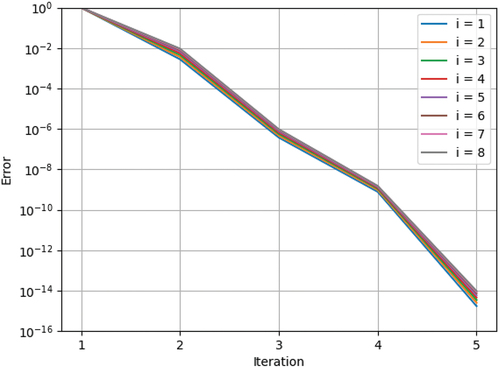
Gauss-Seidel has a low per iteration cost but is difficult to parallelize and converges slowly compared to Krylov subspace methods, so it is not desirable for most modern large-scale numerical analyses. However, the CRAM depletion calculation is inherently parallelizable across independent depletion zones, meaning the linear system solution for each depletion zone does not need to be parallelized. Thus, the inability to parallelize GS is irrelevant for practical depletion analyses using CRAM. Furthermore, the matrices that appear in CRAM are strongly diagonally dominant due to the subtraction of ${\theta }_i$, whose values are orders of magnitude larger than the typical magnitude of physical quantities constituting the depletion matrices, from the diagonal elements. Owing to the strong diagonal dominance, GS exhibits extremely fast convergence for the CRAM matrices, as illustrated in Fig. 1, where the error is defined as the relative $l^2$-norm of the solution change between two iterations. As a result, the number of GS iterations required to reach a sufficient convergence level becomes small enough to make GS potentially cheaper than SGE. To summarize, the unique characteristics of CRAM applied to the depletion analysis make GS a highly compelling option.

Fig. 1. Convergence behavior of GS for each CRAM matrix, examined with CRAM-PFD-AO-16, depletion system with 3307 nuclides and a depletion interval of 1 day.

The convergence of GS can be further improved by introducing the successive over-relaxation method with minimal algorithmic changes and virtually the same computational cost, often by a significant degree for high-spectral-radius problems. However, the extremely fast convergence of GS for the CRAM matrices implies that the spectral radii of all CRAM matrices considered in this work are very close to zero. Therefore, the improvement of the convergence rate by introducing successive over-relaxation will be marginal for CRAM even though optimal relaxation factors are used, which are cumbersome to determine. On the contrary, it can even worsen the spectral radius and deteriorate the convergence of GS in this case if an improper over-relaxation factor is used.

IV. RESULTS

We considered several depletion systems, each with different numbers of nuclides, 1693, 299, and 37. We then determined the run times and made comparisons using the simple standards of maximum nuclide absolute relative difference (MNARD) and average nuclide absolute relative difference (ANARD) as needed. Additionally, CRAM occasionally calculates negative nuclide number densities (NNNDs). When these NNNDs occur, the number of these negative densities is included as this is another metric by which solving CRAM using a given method at a given AO can be judged since negative densities are clearly nonphysical.

Additionally, we considered two different criteria when comparing methods. In one instance, we considered the absolute relative differences (ARDs) of the NNDs of all nuclides in the system, regardless of how small the concentration of the nuclide is. This is intended to investigate the computational robustness of a given method. In another instance, we considered only those nuclides with NNDs greater than ${10}^{-10}$ atoms/b∙cm and with ARDs greater than ${10}^{-4}$. This is intended to investigate the practical applicability of a given method to a real-world analysis where real-world uncertainties and tolerances restrict analyses to two or three significant figures.

The depletion conditions used were a one-group neutron flux of ${10}^{15}$ n/cm²∙s for a period of $8.64\times {10}^6$ s (100 days). These depletion conditions were chosen to both be somewhat represented of the flux levels experienced in thermal reactors as well as challenge CRAM, which is documented as having difficulties modeling fresh fuel systems compared to depleted fuel systems.^[5]

IV.A. 1693 Nuclides

The 1693-nuclide library is generated using decay data from Evaluated Nuclear Data File (ENDF) VIII.0 decay data^[13] and pretabulated one-group cross-section data taken from ORIGEN^[7] data distributed in SCALE 6.2.X versions for beginning-of-life pressurized water reactor fuel at 5% enrichment for a Westinghouse $17\times 17$ assembly. This library is meant to represent the maximum anticipated number of nuclides tracked in depletion calculations. While ENDF provides decay data for 3820 nuclides,^[13] in reality, the lack of cross-section data for many of these nuclides restricts the number of nuclides that can be produced via transmutation in nuclear fission reactors. When SGE was first applied to CRAM, a system using 1606 nuclides was used, which was considered quite comprehensive.^[10]

IV.A.1. Direct Matrix Inversion

For DMI, Griffin uses the LAPACK routine ZGESV to solve linear equations where the matrix inverse is required.^[14] We first compared the results of the various AOs of CRAM compared to the highest AO for which there are published coefficients, AO-48, and solved using DMI. The results of this comparison are shown in Fig. 2 and Tables I and II.

TABLE I DMI Run Times and Results for the 1693-Nuclide Case

AO	Time (ms)	MNARD	ANARD	NNND
4	$357.769\pm 4.963$	$1.16\times {10}^8$	$1.90\times {10}^5$	160
8	$704.775\pm 6.464$	$1.63\times {10}^4$	$4.53\times {10}^1$	75
12	$1049.482\pm 6.112$	$5.47\times {10}^6$	$3.23\times {10}^3$	21
16	$1394.419\pm 9.405$	$3.66\times {10}^0$	$4.71\times {10}^{-3}$	1
20	$1733.940\pm 6.449$	$9.93\times {10}^{-1}$	$1.04\times {10}^{-3}$	0
24	$2079.826\pm 10.398$	$8.84\times {10}^{-1}$	$8.18\times {10}^{-4}$	0
28	$2420.296\pm 9.718$	$6.41\times {10}^0$	$3.95\times {10}^{-3}$	0
32	$2762.308\pm 7.923$	$1.78\times {10}^5$	$1.09\times {10}^2$	0
36	$3069.058\pm 10.340$	$3.08\times {10}^2$	$1.84\times {10}^{-1}$	0
40	$3446.458\pm 13.190$	$1.98\times {10}^2$	$1.17\times {10}^{-1}$	0
44	$3788.330\pm 10.768$	$4.07\times {10}^8$	$2.40\times {10}^5$	1
48	$4077.579\pm 16.048$	—	—	0

TABLE II DMI ARD Results for the 1693-Nuclide Case for Nuclides with NNDs Greater than ${10}^{-10}$ atoms/b∙cm

AO	MNARD	ANARD	NNND
4	$4.89\times {10}^0$	$3.76\times {10}^{-2}$	5
8	$6.17\times {10}^{-3}$	$2.65\times {10}^{-5}$	0
12	$2.71\times {10}^{-6}$	$7.89\times {10}^{-9}$	0
16	$5.00\times {10}^{-10}$	$1.48\times {10}^{-12}$	0
20	$1.07\times {10}^{-12}$	$4.72\times {10}^{-15}$	0
24	$5.72\times {10}^{-5}$	$3.04\times {10}^{-5}$	0
28	$1.07\times {10}^{-12}$	$4.61\times {10}^{-15}$	0
32	$3.42\times {10}^{-13}$	$4.53\times {10}^{-15}$	0
36	$3.25\times {10}^{-12}$	$1.06\times {10}^{-14}$	0
40	$1.07\times {10}^{-12}$	$4.44\times {10}^{-15}$	0
44	$1.96\times {10}^{-12}$	$8.70\times {10}^{-15}$	0
48	-	-	0

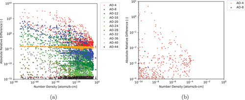
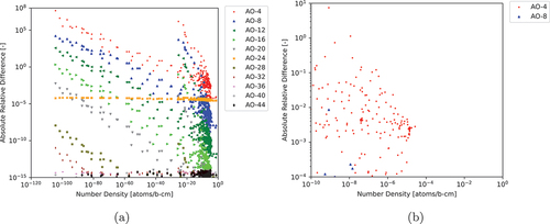
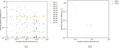
Fig. 2. ARDs between various AOs of CRAM to AO-48 applying DMI (a) for all nuclides and (b) for nuclides with NNDs greater than ${10}^{-10}$ atoms/b∙cm and ARDs greater than ${10}^{-4}$.

Based on these results, we can determine that AO-12 can model nuclides with NNDs greater than ${10}^{-10}$ atoms/b∙cm within an ARD ${10}^{-4}$ compared to AO-48, which has been demonstrated previously to achieve near floating-point double precision.^[11] We also note that as shown in Fig. 2a, there is a numerical instability for several nuclides with NNDs below ${10}^{-20}$ atoms/b∙cm with the results calculated by higher AOs diverging from the AO-48 result. We will investigate this divergence further in Sec. IV.A.2.

IV.A.2. Sparse Gaussian Elimination

We repeated the same process in Sec. IV.A.1 except now applying SGE to CRAM with the results for various AOs shown in Fig. 3 and Tables III and IV.

TABLE III SGE Run Times and Results for the 1693-Nuclide Case

AO	Time (ms)	MNARD	ANARD	NNND
4	$10.973\pm 0.472$	$1.16\times {10}^8$	$1.91\times {10}^5$	160
8	$15.471\pm 0.547$	$1.63\times {10}^4$	$4.54\times {10}^1$	74
12	$20.231\pm 0.962$	$5.82\times {10}^2$	$7.60\times {10}^{-1}$	21
16	$24.380\pm 0.805$	$3.66\times {10}^0$	$3.94\times {10}^{-3}$	1
20	$28.175\pm 0.808$	$1.11\times {10}^{-2}$	$1.09\times {10}^{-5}$	0
24	$33.423\pm 1.022$	$6.80\times {10}^{-5}$	$3.33\times {10}^{-5}$	0
28	$36.585\pm 1.351$	$2.55\times {10}^{-8}$	$2.68\times {10}^{-11}$	0
32	$41.539\pm 1.296$	$2.42\times {10}^{-11}$	$3.25\times {10}^{-14}$	0
36	$45.512\pm 1.648$	$1.17\times {10}^{-14}$	$1.16\times {10}^{-15}$	0
40	$49.883\pm 1.840$	$9.97\times {10}^{-15}$	$6.53\times {10}^{-16}$	0
44	$53.299\pm 1.759$	$1.00\times {10}^{-14}$	$9.30\times {10}^{-16}$	0
48	$58.016\pm 1.428$	—	—	0

TABLE IV SGE ARD Results for the 1693-Nuclide Case for Nuclides Greater than ${10}^{-10}$ atoms/b∙cm

AO	MNARD	ANARD	NNND
4	$4.89\times {10}^0$	$3.76\times {10}^{-2}$	5
8	$6.17\times {10}^{-3}$	$2.65\times {10}^{-5}$	0
12	$2.71\times {10}^{-6}$	$7.86\times {10}^{-9}$	0
16	$5.00\times {10}^{-10}$	$1.45\times {10}^{-12}$	0
20	$5.06\times {10}^{-14}$	$1.26\times {10}^{-15}$	0
24	$5.72\times {10}^{-5}$	$3.04\times {10}^{-5}$	0
28	$1.00\times {10}^{-14}$	$8.57\times {10}^{-16}$	0
32	$1.00\times {10}^{-14}$	$2.60\times {10}^{-15}$	0
36	$9.64\times {10}^{-15}$	$1.04\times {10}^{-15}$	0
40	$9.64\times {10}^{-15}$	$6.01\times {10}^{-16}$	0
44	$1.00\times {10}^{-14}$	$8.29\times {10}^{-16}$	0
48	—	—	0

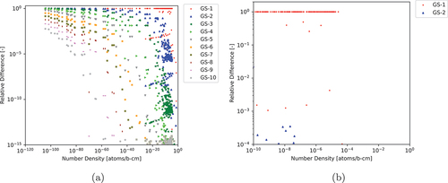
Fig. 3. ARDs between various AOs of CRAM to AO-48 applying SGE (a) for all nuclides and (b) for nuclides with NNDs greater than ${10}^{-10}$ atoms/b∙cm and ARDs greater than ${10}^{-4}$.

Based on the results from Fig. 3b and Table IV, we once again determined that AO-12 is capable of achieving the desired precision for practical modeling purposes.

Unlike DMI, SGE does not exhibit the same numerical instability. However, we cannot conclude that SGE is more accurate than DMI based on this alone. In order to determine which is more accurate, we used the adding and doubling method (ADM) implemented in Griffin^[15] to generate a set of results independent of the results calculated by CRAM and compare both the DMI and SGE results to the results calculated by ADM. ADM with approximation power 25 was used, which, based on previous testing, is expected to achieve a 9- or 10-digit agreement with CRAM-AO-48. The results of this comparison are shown in Fig. 4 and Table V.

TABLE V ARDs Between CRAM-SGE-48 and CRAM-DMI-48 When Compared to ADM-25 for All Nuclides

Method	MNARD	ANARD
SGE	$2.40\times {10}^{-2}$	$1.42\times {10}^{-5}$
DMI	$5.17\times {10}^2$	$3.06\times {10}^{-1}$

Fig. 4. ARDs of CRAM-SGE-48 and CRAM-DMI-48 compared to ADM-25 for the 1693-nuclide case.

Overall, SGE achieves much better agreement with ADM than DMI does, leading to the conclusion that SGE is more accurate than DMI. It should be noted that the system considered in this work corresponds to a fresh fuel case, which CRAM with DMI has been previously documented as experiencing large relative errors for some nuclides with previous research calculating a ²⁴⁶Cm relative error of ${10}^{-6}$.^[5] Only one nuclide has an ARD greater than ${10}^{-8}$ between ADM and SGE, which corresponds to ⁸Be, an extraordinarily short-lived nuclide that ADM has had difficulty modeling.^[15] For the remainder of this work, we will still consider the performance of DMI applied to CRAM for the sake of completeness, but based on the two currently published methods and the results from Tables I and III, we can already confirm the previously published results that CRAM-SGE is superior to CRAM-DMI in terms of both accuracy and run time.

For completeness, we provide information regarding the nuclides for which CRAM-DMI-48 provides NND ARDs greater than ${10}^{-7}$ when compared to the ADM-25 NND solution as shown in Table VI. With the exception of ${ }^8\mathrm{Be}$, which has a remarkably large decay constant as discussed previously, all nuclides that experience large ARDs between CRAM-DMI-48 and ADM-25 can be produced as fission products only from the spontaneous fission of ${ }^{242}\mathrm{Cm}$. Curium-242 has a decay constant of $4.92\times {10}^{-8}$ and a spontaneous fission branching ratio of $6.10\times {10}^{-8}$. Most of the yield fraction terms are on the order of ${10}^{-7}$, which results in the depletion matrix having off-diagonal production terms for the metastable radionuclides in Table VI on the order of ${10}^{-22}$ while the metastable nuclides themselves have diagonal destruction terms between ${10}^{-3}$ to ${10}^3$. This difference of up to 25 orders of magnitude can cause numerical problems when working in double-precision, which occurs when performing the LU decomposition required by DMI. A similar issue is present for ${ }^8\mathrm{Be},$ which is produced via the ${ }^9\mathrm{Be}{\left(\mathrm{n},2\mathrm{n}\right)}^8\mathrm{Be}$ reaction. This production term will be many orders of magnitude smaller than the destruction term of ${ }^8\mathrm{Be}$, once again presenting numerical challenges when using double-precision.

TABLE VI Nuclides with an ARD Greater than ${10}^{-7}$ Between the ADM-25 and CRAM-DMI-48 Solutions for the 1693-Nuclide Case

Nuclide	Decay Constant (s^–1)	Curium-242 Spontaneous Fission Yield	ADM NND (atom/b∙cm)	ARD
${ }^8\mathrm{Be}$	$8.47\times {10}^{15}$	—	$3.26\times {10}^{-37}$	$2.40\times {10}^{-2}$
${ }^{70m2}\mathrm{Cu}$	$0.105$	$2.71\times {10}^{-9}$	$1.41\times {10}^{-29}$	$3.80\times {10}^{-2}$
${ }^{73m1}\mathrm{Zn}$	$0.120$	$3.58\times {10}^{-8}$	$1.64\times {10}^{-28}$	$1.38\times {10}^{-4}$
${ }^{73m2}\mathrm{Zn}$	$53.3$	$2.03\times {10}^{-7}$	$2.09\times {10}^{-30}$	$4.36\times {10}^{-4}$
${ }^{77m}\mathrm{Zn}$	$0.660$	$6.53\times {10}^{-9}$	$5.42\times {10}^{-30}$	$1.39\times {10}^{-2}$
${ }^{117m}\mathrm{Pd}$	$36.3$	$8.37\times {10}^{-8}$	$1.26\times {10}^{-30}$	$1.82\times {10}^{-1}$
${ }^{114m}\mathrm{Ag}$	$462$	$1.24\times {10}^{-4}$	$1.48\times {10}^{-28}$	$3.17\times {10}^{-3}$
${ }^{155m}\mathrm{Gd}$	$21.7$	$2.50\times {10}^{-8}$	$6.34\times {10}^{-31}$	$5.17\times {10}^2$
${ }^{168m}\mathrm{Ho}$	$5.25\times {10}^{-3}$	$1.76\times {10}^{-7}$	$1.84\times {10}^{-26}$	$2.12\times {10}^{-4}$
${ }^{177m}\mathrm{Yb}$	$0.108$	$2.70\times {10}^{-10}$	$1.37\times {10}^{-30}$	$2.37\times {10}^{-7}$

IV.A.3. Gauss-Seidel

We then considered the application of GS to CRAM. Since GS requires a number of iterations to perform, we first considered the performance of GS with a varying number of iterations for AO-48 and compared the results to that of CRAM-SGE-AO-48. The results of these comparisons are shown in Fig. 5 and Tables VII and VIII.

TABLE VII CRAM-AO-48 with GS with Varying Numbers of Iteration Run Times and Results for the 1693-Nuclide Case

GS Iterations	Time (ms)	MNARD	ANARD	NNND
1	$7.267\pm 0.263$	$1.00\times {10}^0$	$9.27\times {10}^{-1}$	139
2	$13.015\pm 0.410$	$1.02\times {10}^0$	$1.09\times {10}^{-1}$	42
3	$18.537\pm 0.458$	$1.25\times {10}^0$	$4.08\times {10}^{-2}$	25
4	$23.747\pm 0.539$	$1.04\times {10}^0$	$2.48\times {10}^{-2}$	5
5	$29.317\pm 0.610$	$9.95\times {10}^{-1}$	$1.22\times {10}^{-2}$	0
6	$34.343\pm 0.730$	$3.43\times {10}^{-1}$	$3.51\times {10}^{-3}$	0
7	$40.494\pm 0.765$	$9.10\times {10}^{-2}$	$6.34\times {10}^{-4}$	0
8	$45.018\pm 0.912$	$1.22\times {10}^{-2}$	$4.66\times {10}^{-5}$	0
9	$50.632\pm 1.134$	$1.74\times {10}^{-3}$	$2.99\times {10}^{-6}$	0
10	$56.140\pm 1.043$	$2.87\times {10}^{-4}$	$2.56\times {10}^{-7}$	0

TABLE VIII CRAM-AO-48 with GS with Varying Numbers of Iteration Results for the 1693-Nuclide Case for Nuclides with NNDs Greater than ${10}^{-10}$ atoms/b∙cm

GS Iterations	MNARD	ANARD	NNND
1	$1.00\times {10}^0$	$9.05\times {10}^{-1}$	90
2	$9.93\times {10}^{-1}$	$7.09\times {10}^{-2}$	0
3	$1.46\times {10}^{-1}$	$1.02\times {10}^{-3}$	0
4	$3.50\times {10}^{-4}$	$1.29\times {10}^{-6}$	0
5	$7.81\times {10}^{-8}$	$1.08\times {10}^{-9}$	0
6	$8.83\times {10}^{-10}$	$6.37\times {10}^{-12}$	0
7	$3.77\times {10}^{-11}$	$1.12\times {10}^{-13}$	0
8	$9.64\times {10}^{-15}$	$7.77\times {10}^{-16}$	0
9	$9.64\times {10}^{-15}$	$6.87\times {10}^{-16}$	0
10	$9.64\times {10}^{-15}$	$6.87\times {10}^{-16}$	0

Fig. 5. ARDs between various numbers of GS iterations for CRAM-AO-48 to CRAM-SGE-AO-48 (a) for all nuclides and (b) for nuclides with NNDs greater than ${10}^{-10}$ atoms/b∙cm and ARDs greater than ${10}^{-4}$.

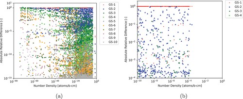
Based on the results, we can determine that even GS-10 does not achieve the same precision as SGE for nuclides with very small NNDs. When considering that GS-10 has a run time of 56 ms compared to the SGE run time of 58 ms from Table III, SGE clearly seems to be the superior method when it comes to computational precision for these low nuclides with very small NNDs. However, as shown in Fig. 5b and Table VIII, GS-5 is capable of achieving an MNARD of less than ${10}^{-4}$ for all nuclides with NNDs greater than ${10}^{-10}$ atoms/b∙cm. Additionally, the run time of CRAM-GS-5-AO-48 is only 29 ms, which is half of the CRAM-SGE-AO-48 run time. This means that for practical modeling purposes, CRAM-GS-5-AO-48 could be used instead of CRAM-SGE-AO-48 and reduce the overall run time of the depletion calculation by 50%. Of course, if we consider practical purposes, Table III also demonstrates that CRAM-SGE-AO-12 is capable of achieving an MNARD of less than ${10}^{-4}$ for nuclides with NND greater than ${10}^{-10}$ atoms/b∙cm with a run time of only 20 ms, which is less than that of CRAM-GS-5-AO-48. Consequently, we then tested the application of GS with a varying number of iterations to CRAM-AO-12 and compared the numerical results with those of CRAM-SGE-AO-48, as shown in Fig. 6 and Tables IX and X.

TABLE IX CRAM-AO-12 with GS with Varying Numbers of Iteration Run Times and ARDs to CRAM-SGE-AO-48 for the 1693-Nuclide Case

GS Iterations	Time (ms)	MNARD	ANARD	NNND
1	$2.780\pm 0.147$	$1.33\times {10}^2$	$1.07\times {10}^0$	149
2	$4.351\pm 0.215$	$5.71\times {10}^2$	$8.93\times {10}^{-1}$	111
3	$5.576\pm 0.231$	$5.73\times {10}^2$	$7.89\times {10}^{-1}$	88
4	$7.084\pm 0.252$	$5.61\times {10}^2$	$9.02\times {10}^{-1}$	57
5	$8.357\pm 0.362$	$5.30\times {10}^2$	$9.31\times {10}^{-1}$	51
6	$9.776\pm 0.337$	$6.59\times {10}^2$	$1.49\times {10}^0$	38
7	$11.351\pm 0.327$	$6.92\times {10}^2$	$1.50\times {10}^0$	30
8	$12.653\pm 0.341$	$7.14\times {10}^2$	$1.12\times {10}^0$	25
9	$13.869\pm 0.349$	$5.82\times {10}^2$	$7.63\times {10}^{-1}$	22
10	$15.153\pm 0.393$	$5.82\times {10}^2$	$7.60\times {10}^{-1}$	21

TABLE X CRAM-AO-12 with GS with Varying Numbers of Iteration ARD to CRAM-SGE-AO-48 for the 1693-Nuclide Case for Nuclides with NNDs Greater than ${10}^{-10}$ atoms/b∙cm

GS Iterations	MNARD	ANARD	NNND
1	$1.00\times {10}^0$	$9.05\times {10}^{-1}$	72
2	$1.08\times {10}^0$	$8.79\times {10}^{-2}$	1
3	$2.30\times {10}^{-1}$	$2.30\times {10}^{-3}$	0
4	$1.80\times {10}^{-3}$	$8.35\times {10}^{-6}$	0
5	$7.38\times {10}^{-6}$	$5.25\times {10}^{-8}$	0
6	$2.81\times {10}^{-6}$	$8.74\times {10}^{-9}$	0
7	$2.71\times {10}^{-6}$	$7.89\times {10}^{-9}$	0
8	$2.71\times {10}^{-6}$	$7.86\times {10}^{-9}$	0
9	$2.71\times {10}^{-6}$	$7.86\times {10}^{-9}$	0
10	$2.71\times {10}^{-6}$	$7.86\times {10}^{-9}$	0

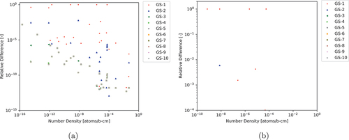
Fig. 6. ARDs between various numbers of GS iterations for CRAM-AO-12 to CRAM-SGE-AO-48 (a) for all nuclides and (b) for nuclides with NNDs greater than ${10}^{-10}$ atoms/b∙cm and ARDs greater than ${10}^{-4}$.

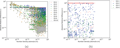
The CRAM-GS-AO-12 results do not converge to the CRAM-SGE-AO-48 result with increasing number of iterations to the same extent that the CRAM-GS-AO-48 results did, but this is to be expected as the results would be expected to converge to the CRAM-SGE-AO-12 results, which achieved limited agreement with CRAM-SGE-AO-48. As shown in Table X, CRAM-GS-5-AO-12 achieves an MNARD of less than ${10}^{-4}$ compared to CRAM-SGE-AO-48 for all nuclides with NNDs greater than ${10}^{-10}$ atoms/b∙cm. The total run time of CRAM-GS-5-AO-12 is 8 ms, which is less than half the run time of CRAM-SGE-AO-12, once again indicating that for practical modeling purposes, CRAM-GS-5-AO-12 can reduce the depletion calculation run time by more than 50% for the 1693-nuclide case.

IV.B. 299 Nuclides

While we have already verified the performance of GS applied to CRAM for a 1693-nuclide library, which is anticipated to be near the upper limit of the number of nuclides tracked in any depletion calculation, we continued our investigation considering smaller nuclide libraries. The motivation for this is that many depletion tools restrict their analysis to a few hundred nuclides or fewer. There are several motivations for this, namely, the desire to avoid tracking extremely short-lived nuclides, which can introduce stiffness to the depletion matrix while having a minimal impact on the depletion calculation. Consequently, the performance of various methods of solving CRAM with varying depletion matrix sizes has practical interest and is investigated here.

The decay and cross-section data used for the 299-nuclide case comes from the DRAGON5^[16] application.

IV.B.1. Direct Matrix Inversion

We repeated the process from Sec. IV.A.1 for the 299-nuclide case, the results of which are shown in Fig. 7 and Tables XI and XII. Unlike Fig. 2, the 299-nuclide case does not exhibit the same numerical instability for a few nuclides when solving CRAM using DMI when compared to the 1693-nuclide case. Because of this lack of instability, we did not perform the same comparison between CRAM-DMI and CRAM-SGE with ADM since there is not inconsistent behavior between the two versions of CRAM.

TABLE XI DMI Run Times and Results for the 299-Nuclide Case

AO	Time (ms)	MNARD	ANARD	NNND
4	$3.414\pm 0.212$	$4.41\times {10}^7$	$1.84\times {10}^5$	29
8	$6.641\pm 0.351$	$1.63\times {10}^4$	$1.68\times {10}^2$	32
12	$9.895\pm 0.357$	$3.74\times {10}^2$	$2.54\times {10}^0$	18
16	$12.960\pm 0.366$	$2.08\times {10}^0$	$1.20\times {10}^{-2}$	1
20	$16.037\pm 0.454$	$5.74\times {10}^{-3}$	$2.99\times {10}^{-5}$	0
24	$19.278\pm 0.367$	$6.78\times {10}^{-5}$	$3.93\times {10}^{-5}$	0
28	$22.072\pm 0.394$	$1.15\times {10}^{-8}$	$5.33\times {10}^{-11}$	0
32	$25.294\pm 0.438$	$1.04\times {10}^{-11}$	$4.92\times {10}^{-14}$	0
36	$28.351\pm 0.509$	$8.74\times {10}^{-15}$	$1.81\times {10}^{-15}$	0
40	$31.359\pm 0.599$	$8.74\times {10}^{-15}$	$5.37\times {10}^{-16}$	0
44	$34.244\pm 0.571$	$9.16\times {10}^{-15}$	$1.81\times {10}^{-15}$	0
48	$37.076\pm 0.486$	—	—	0

TABLE XII DMI Results for the 299-Nuclide Case for Nuclides with NNDs Greater than ${10}^{-10}$ atoms/b∙cm

AO	MNARD	ANARD	NNND
4	$7.45\times {10}^0$	$6.41\times {10}^{-2}$	2
8	$8.57\times {10}^{-3}$	$5.25\times {10}^{-5}$	0
12	$1.73\times {10}^{-6}$	$1.10\times {10}^{-8}$	0
16	$4.10\times {10}^{-11}$	$5.89\times {10}^{-13}$	0
20	$5.73\times {10}^{-14}$	$9.81\times {10}^{-16}$	0
24	$5.30\times {10}^{-5}$	$3.43\times {10}^{-5}$	0
28	$8.74\times {10}^{-15}$	$6.90\times {10}^{-16}$	0
32	$9.16\times {10}^{-15}$	$2.49\times {10}^{-15}$	0
36	$8.74\times {10}^{-15}$	$1.81\times {10}^{-15}$	0
40	$8.74\times {10}^{-15}$	$6.33\times {10}^{-16}$	0
44	$9.16\times {10}^{-15}$	$1.94\times {10}^{-15}$	0
48	—	—	0

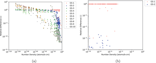
Fig. 7. ARDs between various AOs of CRAM to AO-48 applying DMI (a) for all nuclides and (b) for nuclides with NNDs greater than ${10}^{-10}$ atoms/b∙cm and ARDs greater than ${10}^{-4}$.

Based on the results from Fig. 7b and Table XII, we can determine that AO-12 is suitable for practical modeling purposes, the same as for the 1693-nuclide case.

IV.B.2. Sparse Gaussian Elimination

We repeated the process from Sec. IV.A.2 for the 299-nuclide case, the results of which are shown in Fig. 8 and Tables XIII and XIV.

TABLE XIII SGE Run Times and Results for the 299-Nuclide Case

AO	Time (ms)	MNARD	ANARD	NNND
4	$1.190\pm 0.094$	$4.41\times {10}^7$	$1.84\times {10}^5$	29
8	$1.898\pm 0.121$	$1.63\times {10}^4$	$1.68\times {10}^2$	32
12	$2.579\pm 0.172$	$3.74\times {10}^2$	$2.54\times {10}^0$	18
16	$3.259\pm 0.226$	$2.08\times {10}^0$	$1.20\times {10}^{-2}$	1
20	$4.004\pm 0.252$	$5.74\times {10}^{-3}$	$2.99\times {10}^{-5}$	0
24	$4.716\pm 0.257$	$6.78\times {10}^{-5}$	$3.93\times {10}^{-5}$	0
28	$5.399\pm 0.249$	$1.15\times {10}^{-8}$	$5.33\times {10}^{-11}$	0
32	$6.161\pm 0.323$	$1.04\times {10}^{-11}$	$4.89\times {10}^{-14}$	0
36	$6.720\pm 0.319$	$9.16\times {10}^{-15}$	$1.89\times {10}^{-15}$	0
40	$7.435\pm 0.380$	$9.16\times {10}^{-15}$	$9.52\times {10}^{-16}$	0
44	$8.089\pm 0.323$	$8.94\times {10}^{-15}$	$9.34\times {10}^{-16}$	0
48	$8.698\pm 0.285$	—	—	0

TABLE XIV SGE Run Times and Results for the 299-Nuclide Case for Nuclides with NNDs Greater than ${10}^{-10}$ atoms/b∙cm

AO	MNARD	ANARD	NNND
4	$7.45\times {10}^0$	$6.41\times {10}^{-2}$	2
8	$8.57\times {10}^{-3}$	$5.25\times {10}^{-5}$	0
12	$1.73\times {10}^{-6}$	$1.10\times {10}^{-8}$	0
16	$4.10\times {10}^{-11}$	$5.88\times {10}^{-13}$	0
20	$5.85\times {10}^{-14}$	$1.33\times {10}^{-15}$	0
24	$5.30\times {10}^{-5}$	$3.43\times {10}^{-5}$	0
28	$8.74\times {10}^{-15}$	$7.61\times {10}^{-16}$	0
32	$8.81\times {10}^{-15}$	$2.09\times {10}^{-15}$	0
36	$9.16\times {10}^{-15}$	$1.95\times {10}^{-15}$	0
40	$9.16\times {10}^{-15}$	$1.13\times {10}^{-15}$	0
44	$8.71\times {10}^{-15}$	$9.72\times {10}^{-16}$	0
48	—	—	0

Fig. 8. ARDs between various AOs of CRAM to AO-48 applying SGE (a) for all nuclides and (b) for nuclides with NND greater than ${10}^{-10}$ atoms/b∙cm and ARDs greater than ${10}^{-4}$.

IV.B.3. Gauss-Seidel

Once again, we considered the performance of GS with varying number of iterations applied to CRAM-AO-48, with the results shown in Fig. 9 and Tables XV and XVI.

TABLE XV CRAM-AO-48 with GS with Varying Numbers of Iteration Run Times and Results for the 299-Nuclide Case

GS Iterations	Time (ms)	MNARD	ANARD	NNND
1	$1.251\pm 0.079$	$1.00\times {10}^0$	$8.78\times {10}^{-1}$	0
2	$2.266\pm 0.134$	$1.00\times {10}^0$	$1.13\times {10}^{-1}$	0
3	$3.241\pm 0.187$	$1.02\times {10}^0$	$7.03\times {10}^{-2}$	3
4	$4.181\pm 0.181$	$9.74\times {10}^{-1}$	$3.91\times {10}^{-2}$	0
5	$5.268\pm 0.173$	$6.28\times {10}^{-1}$	$1.78\times {10}^{-2}$	0
6	$6.215\pm 0.231$	$3.10\times {10}^{-1}$	$7.10\times {10}^{-3}$	0
7	$7.286\pm 0.252$	$1.42\times {10}^{-1}$	$2.60\times {10}^{-3}$	0
8	$8.090\pm 0.273$	$5.82\times {10}^{-2}$	$8.60\times {10}^{-4}$	0
9	$9.081\pm 0.259$	$2.06\times {10}^{-2}$	$2.50\times {10}^{-4}$	0
10	$10.082\pm 0.330$	$5.82\times {10}^{-3}$	$6.08\times {10}^{-5}$	0

TABLE XVI CRAM-AO-48 with GS with Varying Numbers of Iteration Results for the 299-Nuclide Case for Nuclides with NNDs Greater than ${10}^{-10}$ atoms/b∙cm

GS Iterations	MNARD	ANARD	NNND
1	$1.00\times {10}^0$	$8.87\times {10}^{-1}$	0
2	$3.49\times {10}^{-4}$	$1.56\times {10}^{-5}$	0
3	$2.50\times {10}^{-9}$	$6.81\times {10}^{-11}$	0
4	$9.38\times {10}^{-15}$	$7.68\times {10}^{-16}$	0
5	$9.16\times {10}^{-15}$	$8.28\times {10}^{-16}$	0
6	$9.16\times {10}^{-10}$	$8.28\times {10}^{-12}$	0
7	$9.16\times {10}^{-11}$	$8.28\times {10}^{-13}$	0
8	$9.16\times {10}^{-15}$	$8.28\times {10}^{-16}$	0
9	$9.16\times {10}^{-15}$	$8.28\times {10}^{-16}$	0
10	$9.16\times {10}^{-15}$	$8.28\times {10}^{-16}$	0

Fig. 9. ARDs between various numbers of GS iterations for CRAM-AO-48 to CRAM-SGE-AO-48 (a) for all nuclides and (b) for nuclides with NNDs greater than ${10}^{-10}$ atoms/b∙cm and ARDs greater than ${10}^{-4}$.

Interestingly, unlike in Sec. IV.A.3, CRAM-GS-3-AO-48 is able to achieve an MNARD of less than ${10}^{-4}$ for nuclides with NNDs greater than ${10}^{-10}$ atoms/b∙cm. This indicates that the 299-nuclide case is easier to converge, and thus, fewer GS iterations are required to achieve the desired agreement based on the given criteria. However, we show in Fig. 9a and Table XV that even GS-10 cannot achieve convergence with CRAM-SGE-AO-48 for nuclides with very low NNDs, and based on the trends exhibited in Fig. 9a, it would likely take GS-20 or GS-30 to achieve the same level of agreement between CRAM-GS-AO-48 and CRAM-SGE-AO-48 compared to CRAM-SGE-AO-44.

Turning back to the practical case, CRAM-GS-3-AO-48 has a run time of only 3 ms, which is almost one-third of the 8.7-ms run time of CRAM-SGE-AO-48. However, once again, we consider that CRAM-SGE-AO-12 achieves a ${10}^{-4}$ agreement for nuclides with NNDs greater than ${10}^{-10}$ atoms/b∙cm with a run time of only 2.6 ms. Thus, we consider CRAM-GS-AO-12 with varying numbers of iterations as shown in Fig. 10 and Tables XVII and XVIII. The results demonstrated that CRAM-GS-3-AO-12 is able to achieve the desired ${10}^{-4}$ agreement for nuclides with NNDs greater than ${10}^{-10}$ atoms/b∙cm with a run time of only 0.96 ms, which is roughly one-third the run time of CRAM-SGE-AO-12.

TABLE XVII CRAM-AO-12 with GS with Varying Numbers of Iteration Run Times and ARDs to CRAM-SGE-AO-48 for the 299-Nuclide Case

GS Iterations	Time (ms)	MNARD	ANARD	NNND
1	$0.464\pm 0.028$	$3.99\times {10}^1$	$1.08\times {10}^0$	4
2	$0.721\pm 0.048$	$4.00\times {10}^1$	$3.49\times {10}^{-1}$	5
3	$0.960\pm 0.063$	$4.00\times {10}^1$	$3.20\times {10}^{-1}$	25
4	$1.179\pm 0.082$	$4.00\times {10}^1$	$3.09\times {10}^{-1}$	19
5	$1.459\pm 0.091$	$4.00\times {10}^1$	$5.85\times {10}^{-1}$	20
6	$1.703\pm 0.097$	$6.74\times {10}^1$	$1.35\times {10}^0$	19
7	$1.941\pm 0.116$	$3.11\times {10}^2$	$2.91\times {10}^0$	19
8	$2.152\pm 0.143$	$2.39\times {10}^2$	$2.28\times {10}^0$	22
9	$2.387\pm 0.150$	$1.14\times {10}^2$	$2.05\times {10}^0$	21
10	$2.584\pm 0.155$	$1.32\times {10}^2$	$2.66\times {10}^0$	21

TABLE XVIII CRAM-AO-12 with GS with Varying Numbers of Iteration ARDs to CRAM-SGE-AO-48 for the 299-Nuclide Case for Nuclides with NNDs Greater than ${10}^{-10}$ atoms/b∙cm

GS Iterations	MNARD	ANARD	NNND
1	$1.00\times {10}^0$	$8.87\times {10}^{-1}$	0
2	$2.12\times {10}^{-3}$	$6.56\times {10}^{-5}$	0
3	$1.73\times {10}^{-6}$	$1.22\times {10}^{-8}$	0
4	$1.73\times {10}^{-6}$	$1.10\times {10}^{-8}$	0
5	$1.73\times {10}^{-6}$	$1.10\times {10}^{-8}$	0
6	$1.73\times {10}^{-6}$	$1.10\times {10}^{-8}$	0
7	$1.73\times {10}^{-6}$	$1.10\times {10}^{-8}$	0
8	$1.73\times {10}^{-6}$	$1.10\times {10}^{-8}$	0
9	$1.73\times {10}^{-6}$	$1.10\times {10}^{-8}$	0
10	$1.73\times {10}^{-6}$	$1.10\times {10}^{-8}$	0

Fig. 10. ARDs between various numbers of GS iterations for CRAM-AO-12 to CRAM-SGE-AO-48 (a) for all nuclides and (b) for nuclides with NNDs greater than ${10}^{-10}$ atoms/b∙cm and ARDs greater than ${10}^{-4}$.

IV.C. 37 Nuclides

We then considered a 37-nuclide case, representing a very small number of nuclides meant to approximate the fewest nuclides expected to be tracked when performing most depletion calculations.

IV.C.1. Direct Matrix Inversion

Once again, we compared the run times of CRAM-DMI at varying AOs as well as the differences in the results of the various AOs compared to CRAM-DMI-AO-48. The results are shown in Figs. 11a and 11b and Tables XIX and XX. No numerical instability is seen for the 37-nuclide case for DMI.

TABLE XIX DMI Run Times and Results for the 37-Nuclide Case

AO	Time (ms)	MNARD	ANARD	NNND
4	$0.068\pm 0.007$	$2.37\times {10}^2$	$9.22\times {10}^0$	6
8	$0.118\pm 0.008$	$1.52\times {10}^0$	$4.87\times {10}^{-2}$	1
12	$0.164\pm 0.012$	$1.55\times {10}^{-3}$	$4.61\times {10}^{-5}$	0
16	$0.211\pm 0.014$	$5.94\times {10}^{-7}$	$1.70\times {10}^{-8}$	0
20	$0.257\pm 0.018$	$1.10\times {10}^{-10}$	$3.22\times {10}^{-12}$	0
24	$0.301\pm 0.017$	$6.05\times {10}^{-5}$	$3.78\times {10}^{-5}$	0
28	$0.346\pm 0.022$	$4.93\times {10}^{-15}$	$4.88\times {10}^{-16}$	0
32	$0.387\pm 0.020$	$9.80\times {10}^{-15}$	$2.98\times {10}^{-15}$	0
36	$0.436\pm 0.025$	$5.83\times {10}^{-15}$	$1.60\times {10}^{-15}$	0
40	$0.478\pm 0.022$	$5.69\times {10}^{-15}$	$1.23\times {10}^{-15}$	0
44	$0.521\pm 0.025$	$5.75\times {10}^{-15}$	$1.73\times {10}^{-15}$	0
48	$0.562\pm 0.028$	—	—	0

TABLE XX DMI Results for the 37-Nuclide Case for Nuclides with NNDs Greater than ${10}^{-10}$ atoms/b∙cm

AO	MNARD	ANARD	NNND
4	$1.14\times {10}^0$	$8.56\times {10}^{-2}$	1
8	$8.92\times {10}^{-4}$	$4.20\times {10}^{-5}$	0
12	$4.74\times {10}^{-8}$	$3.50\times {10}^{-9}$	0
16	$3.21\times {10}^{-11}$	$1.66\times {10}^{-12}$	0
20	$5.69\times {10}^{-15}$	$6.42\times {10}^{-16}$	0
24	$4.90\times {10}^{-5}$	$3.39\times {10}^{-5}$	0
28	$2.76\times {10}^{-15}$	$2.97\times {10}^{-16}$	0
32	$9.80\times {10}^{-15}$	$3.26\times {10}^{-15}$	0
36	$5.69\times {10}^{-15}$	$1.68\times {10}^{-15}$	0
40	$5.69\times {10}^{-15}$	$1.40\times {10}^{-15}$	0
44	$5.75\times {10}^{-15}$	$1.88\times {10}^{-15}$	0
48	—	—	0

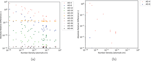
Fig. 11. ARDs between various AOs of CRAM to AO-48 applying DMI (a) for all nuclides and (b) for nuclides with NNDs greater than ${10}^{-10}$ atoms/b∙cm and ARDs greater than ${10}^{-4}$.

IV.C.2. Sparse Gaussian Elimination

As before, we repeated the process for CRAM-SGE for the 37-nuclide case. The results are shown in Fig. 12 and Tables XXI and XXII.

TABLE XXI SGE Run Times and Results for the 37-Nuclide Case

AO	Time (ms)	MNARD	ANARD	NNND
4	$0.058\pm 0.006$	$2.37\times {10}^2$	$9.22\times {10}^0$	6
8	$0.085\pm 0.005$	$1.52\times {10}^0$	$4.87\times {10}^{-2}$	1
12	$0.113\pm 0.009$	$1.55\times {10}^{-3}$	$4.61\times {10}^{-5}$	0
16	$0.143\pm 0.009$	$5.94\times {10}^{-7}$	$1.70\times {10}^{-8}$	0
20	$0.173\pm 0.012$	$1.10\times {10}^{-10}$	$3.22\times {10}^{-12}$	0
24	$0.201\pm 0.014$	$6.05\times {10}^{-5}$	$3.78\times {10}^{-5}$	0
28	$0.228\pm 0.014$	$2.18\times {10}^{-15}$	$5.32\times {10}^{-16}$	0
32	$0.254\pm 0.014$	$5.75\times {10}^{-15}$	$2.94\times {10}^{-15}$	0
36	$0.284\pm 0.018$	$5.83\times {10}^{-15}$	$1.30\times {10}^{-15}$	0
40	$0.313\pm 0.016$	$4.47\times {10}^{-15}$	$8.33\times {10}^{-16}$	0
44	$0.346\pm 0.021$	$5.75\times {10}^{-15}$	$1.80\times {10}^{-15}$	0
48	$0.367\pm 0.019$	—	—	0

TABLE XXII SGE Results for the 37-Nuclide Case for Nuclides with NNDs Greater than ${10}^{-10}$ atoms/b∙cm

AO	MNARD	ANARD	NNND
4	$1.14\times {10}^0$	$8.56\times {10}^{-2}$	1
8	$8.92\times {10}^{-4}$	$4.20\times {10}^{-5}$	0
12	$4.74\times {10}^{-8}$	$3.50\times {10}^{-9}$	0
16	$3.21\times {10}^{-11}$	$1.66\times {10}^{-12}$	0
20	$5.69\times {10}^{-15}$	$6.42\times {10}^{-16}$	0
24	$4.90\times {10}^{-5}$	$3.39\times {10}^{-5}$	0
28	$2.76\times {10}^{-15}$	$2.97\times {10}^{-16}$	0
32	$9.80\times {10}^{-15}$	$3.26\times {10}^{-15}$	0
36	$5.69\times {10}^{-15}$	$1.68\times {10}^{-15}$	0
40	$5.69\times {10}^{-15}$	$1.40\times {10}^{-15}$	0
44	$5.75\times {10}^{-15}$	$1.88\times {10}^{-15}$	0
48	—	—	0

Fig. 12. ARDs between various AOs of CRAM to AO-48 applying SGE (a) for all nuclides and (b) for nuclides with NNDs greater than ${10}^{-10}$ atoms/b∙cm and ARDs greater than ${10}^{-4}$.

IV.C.3. Gauss-Seidel

We then considered varying the number of iterations for CRAM-GS-AO-48. The results are shown in Fig. 13 and Tables XXIII and XXIV. Once again, we observed that GS-3 is able to satisfy the criterion of an MNARD of less than ${10}^{-4}$ for NNDs greater than ${10}^{-10}$ atoms/b∙cm with a run time of 0.204 ms, which is slightly more than half the run time of CRAM-SGE-AO-48, which is 0.367 ms. However, we once again note that CRAM-SGE-AO-12 also satisfies this criterion; thus, we once again applied GS to CRAM-AO-12. The results are shown in Fig. 14 and Tables XXV and XXVI. As shown, CRAM-GS-3-AO-12 is able to achieve the desired agreement with CRAM-SGE-AO-48 with a run time of 0.063 ms compared to the run time of 0.113 ms for CRAM-SGE-AO-12. This once again demonstrates that applying GS to CRAM can yield faster results than SGE while still achieving reasonable accuracy for practical modeling purposes.

TABLE XXIII CRAM-AO-48 with GS with Varying Numbers of Iteration Run Times and Results for the 37-Nuclide Case

GS Iterations	Time (ms)	MNARD	ANARD
1	$0.079\pm 0.006$	$1.00\times {10}^0$	$3.37\times {10}^{-1}$
2	$0.144\pm 0.011$	$1.63\times {10}^{-3}$	$9.01\times {10}^{-5}$
3	$0.204\pm 0.013$	$5.23\times {10}^{-8}$	$2.81\times {10}^{-9}$
4	$0.264\pm 0.015$	$3.68\times {10}^{-12}$	$1.73\times {10}^{-13}$
5	$0.323\pm 0.017$	$2.18\times {10}^{-15}$	$2.90\times {10}^{-16}$
6	$0.384\pm 0.020$	$2.18\times {10}^{-15}$	$2.90\times {10}^{-16}$
7	$0.450\pm 0.024$	$2.18\times {10}^{-15}$	$2.90\times {10}^{-16}$
8	$0.516\pm 0.025$	$2.18\times {10}^{-15}$	$2.90\times {10}^{-16}$
9	$0.572\pm 0.028$	$2.18\times {10}^{-15}$	$2.90\times {10}^{-16}$
10	$0.643\pm 0.030$	$2.18\times {10}^{-15}$	$2.90\times {10}^{-16}$

TABLE XXIV CRAM-AO-48 with GS with Varying Numbers of Iteration Results for the 37-Nuclide Case for Nuclides with NNDs Greater than ${10}^{-10}$ atoms/b∙cm

GS Iterations	MNARD	ANARD
1	$1.00\times {10}^0$	$3.85\times {10}^{-1}$
2	$1.63\times {10}^{-3}$	$6.30\times {10}^{-5}$
3	$6.75\times {10}^{-10}$	$2.61\times {10}^{-11}$
4	$2.18\times {10}^{-15}$	$3.40\times {10}^{-16}$
5	$2.18\times {10}^{-15}$	$3.91\times {10}^{-16}$
6	$2.18\times {10}^{-15}$	$3.91\times {10}^{-16}$
7	$2.18\times {10}^{-15}$	$3.91\times {10}^{-16}$
8	$2.18\times {10}^{-15}$	$3.91\times {10}^{-16}$
9	$2.18\times {10}^{-15}$	$3.91\times {10}^{-16}$
10	$2.18\times {10}^{-15}$	$3.91\times {10}^{-16}$

TABLE XXV CRAM-AO-12 with GS with Varying Numbers of Iteration Run Times and Results for the 37-Nuclide Case

GS Iterations	Time (ms)	MNARD	ANARD
1	$0.030\pm 0.002$	$1.00\times {10}^0$	$3.37\times {10}^{-1}$
2	$0.047\pm 0.003$	$5.94\times {10}^{-3}$	$3.75\times {10}^{-4}$
3	$0.063\pm 0.007$	$1.55\times {10}^{-3}$	$4.62\times {10}^{-5}$
4	$0.075\pm 0.006$	$1.55\times {10}^{-3}$	$4.61\times {10}^{-5}$
5	$0.090\pm 0.006$	$1.55\times {10}^{-3}$	$4.61\times {10}^{-5}$
6	$0.106\pm 0.008$	$1.55\times {10}^{-3}$	$4.61\times {10}^{-5}$
7	$0.123\pm 0.010$	$1.55\times {10}^{-3}$	$4.61\times {10}^{-5}$
8	$0.135\pm 0.009$	$1.55\times {10}^{-3}$	$4.61\times {10}^{-5}$
9	$0.148\pm 0.010$	$1.55\times {10}^{-3}$	$4.61\times {10}^{-5}$
10	$0.166\pm 0.011$	$1.55\times {10}^{-3}$	$4.61\times {10}^{-5}$

TABLE XXVI CRAM-AO-12 with GS with Varying Numbers of Iteration Results for the 37-Nuclide Case for Nuclides with NNDs Greater than ${10}^{-10}$ atoms/b∙cm

GS Iterations	MNARD	ANARD
1	$1.00\times {10}^0$	$3.85\times {10}^{-1}$
2	$5.94\times {10}^{-3}$	$2.29\times {10}^{-4}$
3	$4.74\times {10}^{-8}$	$3.90\times {10}^{-9}$
4	$4.74\times {10}^{-8}$	$3.50\times {10}^{-9}$
5	$4.74\times {10}^{-8}$	$3.50\times {10}^{-9}$
6	$4.74\times {10}^{-8}$	$3.50\times {10}^{-9}$
7	$4.74\times {10}^{-8}$	$3.50\times {10}^{-9}$
8	$4.74\times {10}^{-8}$	$3.50\times {10}^{-9}$
9	$4.74\times {10}^{-8}$	$3.50\times {10}^{-9}$
10	$4.74\times {10}^{-8}$	$3.50\times {10}^{-9}$

Fig. 13. ARDs between various numbers of GS iterations for CRAM-AO-48 to CRAM-SGE-AO-48 (a) for all nuclides and (b) for nuclides with NNDs greater than ${10}^{-10}$ atoms/b∙cm and ARDs greater than ${10}^{-4}$.

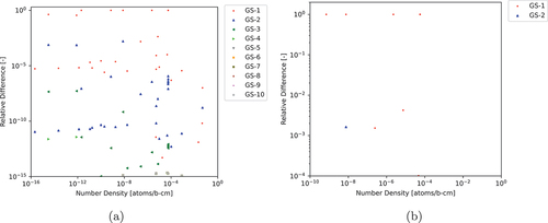
Fig. 14. CRAM-AO-12 with GS with varying numbers of iteration ARDs to CRAM-SGE-AO-48 for the 37-nuclide case for nuclides with NNDs greater than ${10}^{-10}$ atoms/b∙cm.

V. CONCLUSION

We have demonstrated that GS is a viable alternative to solving the linear equations in CRAM than the previously published DMI and SGE methods. When compared to the results calculated by CRAM-SGE-AO-48, GS was able to achieve an agreement of ${10}^{-4}$ for all NNDs greater than ${10}^{-10}$ atoms/b∙cm with a run time roughly half that of the equivalent SGE solution at the same AO. When considering that full-core depletion calculations may involve solving the CRAM equations potentially billions of times, a run-time reduction of 50% could result in hours or potentially days of saved run time. While we have considered only one specific depletion condition (which CRAM was expected to have some challenge solving) for three different nuclide libraries, we anticipate that the reduction in run time and overall accuracy of the solution would be similar for other nuclide libraries with different depletion conditions; however, analysts seeking to use GS should consider performing a cursory comparison between GS and SGE in order to verify that the observed differences are acceptable for their specific use case for nuclides of interest.

Additionally, throughout the course of this work, we have demonstrated that the performance gap between DMI and SGE decreases as the number of nuclides decreases. This expounds on the original CRAM-SGE publication, which demonstrated that SGE was a factor of 10 faster for a specific nuclide library. This work reproduces similar results for large depletion matrices while also demonstrating that the performance gap between DMI and SGE decreases as the number of nuclides in the system decreases. Consequently, developers of depletion-capable applications should not expect a factor of 10 performance improvement when replacing DMI with SGE in their CRAM implementation for all possible depletion problems. Rather, the factor of 10 improvement is the maximum possible run-time improvement when replacing DMI with SGE for CRAM. It is also possible that for incredibly small matrices, such as $3\times 3$, DMI may be faster than SGE, but such depletion systems are unlikely to be encountered when performing practical depletion analysis, and even when encountered, the run time needed to solve the CRAM equations for such a small system would be quite insignificant regardless of the method employed.

Last, we note that the convergence of the 1693-nuclide case with GS is much slower than for the 299- and 37-nuclide cases. This can be clearly seen by comparing Table VIII to Tables XVI and XXIV. We attribute this to the existence of very short-lived radionuclides in the 1693-nuclide case, which are not present in the 299- and 37-nuclide cases with the shortest-lived radionuclides in each library shown in Table XXVII. These short-lived radionuclides result in large decay constant terms on the diagonal of the depletion matrix for the radionuclide itself as well as large negative decay constant terms on the off-diagonals of the decay products of these short-lived radionuclides. This can reduce the diagonal dominance of the depletion matrix, thereby degrading the convergence of GS. However, more research is needed to investigate and quantify the impact of these short-lived radionuclides

TABLE XXVII Shortest-Lived Radionuclides for Each Nuclide Library Tested

Nuclide Case	Nuclide Name	Decay Constant (s^–1)
1693	${ }^8\mathrm{Be}$	$8.47\times {10}^{15}$
299	${ }^{105}\mathrm{Ru}$	$4.34\times {10}^{-5}$
37	${ }^{242}\mathrm{Am}$	$1.20\times {10}^{-5}$

The run times of the CRAM-AO-48 and CRAM-AO-12 results for various nuclide libraries are shown for DMI, SGE, and GS-3 in Table XXVIII and demonstrate the reduced run time of GS-3 compared to SGE and DMI for all cases considered.

TABLE XXVIII Run Times of CRAM Configurations Using DMI, SGE, and GS-3

CRAM Option	1693-Nuclide Time (ms)	299-Nuclide Time (ms)	37-Nuclide Time (ms)
DMI-AO-48	$4077.579\pm 16.048$	$37.076\pm 0.486$	$0.562\pm 0.028$
DMI-AO-12	$1049.482\pm 6.112$	$9.895\pm 0.357$	$0.164\pm 0.012$
SGE-AO-48	$58.016\pm 1.428$	$8.698\pm 0.285$	$0.367\pm 0.019$
SGE-AO-12	$20.231\pm 0.962$	$2.579\pm 0.172$	$0.113\pm 0.009$
GS-3-AO-48	$18.537\pm 0.458$	$3.241\pm 0.187$	$0.204\pm 0.013$
GS-3-AO-12	$5.576\pm 0.231$	$0.960\pm 0.063$	$0.063\pm 0.007$

Acronyms

ADM:	=	adding and doubling method
ANARD:	=	average nuclide absolute relative difference
AO:	=	approximation order
ARD:	=	absolute relative difference
CRAM:	=	Chebyshev Rational Approximation Method
DMI:	=	direct matrix inversion
ENDF:	=	Evaluated Nuclear Data File
GS:	=	Gauss-Seidel
IPF:	=	incomplete partial fraction
MNARD:	=	maximum nuclide absolute relative difference
NND:	=	nuclide number density
NNND:	=	negative nuclide number density.
PFD:	=	partial fraction decomposition
SGE:	=	sparse Gaussian elimination

Acknowledgments

The authors would like to thank Yaqi Wang for their support in implementing this functionality in Griffin.

Disclosure Statement

No potential conflict of interest was reported by the author(s).

Additional information

Funding

This work was funded at Idaho National Laboratory under the Nuclear Energy Advanced Modeling and Simulation program managed by the U.S. Department of Energy Office of Nuclear Energy, under the U.S. Department of Energy Idaho Operations Office contract DE-AC07-05ID14517. Accordingly, the U.S. Government retains a nonexclusive, royalty-free license to publish or reproduce the published form of this contribution, or allow others to do so, for U.S. Government purposes.

References

- H. BATEMAN, “Solution of a System of Differential Equations Occurring in the Theory of Radioactive Transformations,” Proc. Cambridge Philos. Soc. Math. Phys. Sci., 15, 423 (1910).
- G. I. BELL and S. GLASSTONE, Nuclear Reactor Theory, Litton Educational Publishing, Inc. (1970).
- M. PUSA and J. LEPPÄNEN, “Computing the Matrix Exponential in Burnup Calculations,” Nucl. Sci. Eng., 164, 2, 140 (2010); https://doi.org/10.13182/NSE09-14.
- C. MOLER and C. V. LOAN, “Nineteen Dubious Ways to Compute the Exponential of a Matrix, Twenty-Five Years Later,” Soc. Ind. Appl. Math. Rev., 45, 1, 3 (2003).
- M. PUSA, “Rational Approximations to the Matrix Exponential in Burnup Calculations,” Nucl. Sci. Eng., 169, 2, 155 (2011); https://doi.org/10.13182/NSE10-81.
- J. LEPPÄNEN et al., “The Serpent Monte Carlo Code: Status, Development and Applications in 2013,” Ann. Nucl. Energy, 82, 142 (2015); https://doi.org/10.1016/j.anucene.2014.08.024.
- O. W. HERMANN and R. M. WESTFALL, “ORIGEN-S: SCALE System Module to Calculate Fuel Depletion, Actinide Transmutation, Fission Product Buildup and Decay, and Associated Radiation Source Terms,” in “SCALE: A Modular Code System for Performing Standardized Computer Analyses for Licensing Evaluation,” NUREG/CR-0200, Vol II, Sec. F7, Oak Ridge National Laboratory (1998).
- C. H. LEE et al., “Griffin Software Development Plan,” INL/EXT- 21-63185, ANL/NSE-21/23, Idaho National Laboratory/Argonne National Laboratory (2021).
- O. CALVIN et al., “Implementation of Depletion Architecture in the MAMMOTH Reactor Physics Application,” Proc. 2019 Int. Conf. Mathematics and Computational Methods Applied to Nuclear Science and Engineering, Portland, Oregon, August 25–29, 2019, p. 2806, American Nuclear Society (2019).
- M. PUSA and J. LEPPÄNEN, “Solving Linear Systems with Sparse Gaussian Elimination in the Chebyshev Rational Approximation Method,” Nucl. Sci. Eng., 175, 3, 250 (2013); https://doi.org/10.13182/NSE12-52.
- M. PUSA, “Higher-Order Chebyshev Rational Approximation Method and Application to Burnup Equations,” Nucl. Sci. Eng., 182, 3, 297 (2016); https://doi.org/10.13182/NSE15-26.
- O. CALVIN, S. SCHUNERT, and B. GANAPOL, “Global Error Analysis of the Chebyshev Rational Approximation Method,” Ann. Nucl. Energy, 150, 107828 (2021); https://doi.org/10.1016/j.anucene.2020.107828.
- D. A. BROWN et al., “ENDF/B-VIII.0: The 8th Major Release of the Nuclear Reaction Data Library with CIELO-Project Cross Sections, New Standards and Thermal Scattering Data,” Nucl. Data Sheets, 148, 1 (2018); https://doi.org/10.1016/j.nds.2018.02.001.
- E. ANDERSON et al., LAPACK Users’ Guide, Society for Industrial and Applied Mathematics, Philadelphia, Pennsylvania (1999).
- O. W. CALVIN, B. D. GANAPOL, and R. A. BORRELLI, “Introduction of the Adding and Doubling Method for Solving Bateman Equations for Nuclear Fuel Depletion,” Nucl. Sci. Eng., 197, 558 (2023); https://doi.org/10.1080/00295639.2022.2129950.
- G. MARLEAU et al., “A User Guide for DRAGON Version 5,” User Manual IGE-355, Ecole Polytechnique de Montreal (2018).