Analysis of the Operational and Safety Features of the In-Core Bubbling System of the Molten Salt Fast Reactor

Abstract

A foreseen feature of the Molten Salt Fast Reactor is the adoption of a bubbling system for the removal of gaseous and metallic fission products (FPs). This mechanism injects helium bubbles into the core to remove FPs from the salt through floating and mass transfer mechanisms for metallic and gaseous FPs, respectively. The present work is aimed at analyzing this helium bubbling system, focusing on gaseous FPs. We investigate both operational and safety-related features in order to get information useful for the design and to assess the convenience of its adoption. Accordingly, our investigations split into two strands: (1) analyzing the characteristics of the bubbling system itself and (2) assessing the safety features of the reactor in its presence. In order to perform the above analyses, we add the capability to simulate production, transport, and mass transfer of an arbitrary number of gaseous FPs to a preexisting multiphysics solver, built with the OpenFOAM suite. In terms of operational characterization, our analyses quantify the removal efficiency through a characteristic removal time and estimate the poisoning effect of gaseous FPs. In addition, we evaluate the activity and decay heat of the removed gas, which is an aspect crucial for the design of the off-gas unit, and the effect of the bubbling system on the power versus the fuel mass flow rate curve, which is a possible control mechanism. Among our safety-related studies, we first evaluate the void coefficient, determining upper bounds on the helium flow rate in order to avoid prompt supercriticality in case of prompt loss of helium injection. The latter accidental scenario is also analyzed considering the thermal-hydraulic dynamics of the system. We also discuss another accident: complete loss of helium removal.

Keywords:

• Molten Salt Fast Reactor
• passive safety
• in-core bubbling system
• computational fluid dynamics

I. INTRODUCTION

Analysis of the safety features of the Molten Salt Fast Reactor (MSFR) is the grand objective of the European H2020 SAMOSAFER Project (https://samosafer.eu/). Such an objective requires the ability to perform accurate predictions of the behavior of the system both in normal operation and during transients, including accidental ones. Since the design of the MSFR is at an early stage, this kind of analysis is usually carried out with appropriate simulation tools for which the verification and validation activity is ongoing.^[1]

This modeling effort is required considering the different peculiarities characterizing the MSFR with respect to other reactor concepts.^[2] The liquid nature of the fuel, the internal heat generation, the precursors and fission product (FP) transport in the fuel-coolant mixture, and the use of a high-Prandtl-number and high-temperature molten salt are just few of them. The existing simulation tools, mainly developed for the analysis of systems of current industrial interest, i.e., water reactors, are then not suitable for the description of the MSFR.

Given the lack of a physical barrier between the FPs and the molten salt, the FPs can be transported along the circuit. In the current design of the MSFR, an in-core helium injection system^[3] is devised for the removal of FPs. An inert gas, i.e., helium, is injected into the core, thus having contact with the fuel mixture, in order to remove (1) insoluble gaseous FPs via dilution in the gas bubble and (2) metallic particles through capillarity sticking to the bubble. Such a system allows one to remove FPs on line, i.e., without having to stock the fuel mixture in some facility outside the reactor.

The idea of having an off-gas system for removing FPs is not new^[4] since the Molten Salt Reactor Experiment (MSRE) foresaw a system to extract xenon and krypton from the core. However, in the MSRE the FP extraction was performed out-of-core, in the fuel pump bowl where the fuel salt was sprayed into an inert, helium atmosphere. Nonetheless, some gas bubbles were present in the fuel circuit during normal operation contributing to the xenon removal from the core.^[5]

Despite the Xe and Kr poisoning being less concerning in a fast system, the design of the MSFR adopts an in-core extraction, where the helium stream is injected directly into the core region, so that during their flow, FPs can migrate into the bubbles, thereby being removed. This choice entails a better extraction efficiency, both for gaseous and metallic particles, not only improving neutron economy but also bringing benefits in terms of salt chemistry and metal particle deposition issues. On the other hand, an in-core system is more “invasive” from both an operational and a safety point of view. The presence of bubbles causes a nonnegligible void fraction in the active region of the reactor, affecting the neutronics of the system.^[6] This is not a safety issue during normal operation, given the strongly negative void coefficient of the MSFR—possibly considering the helium injected as a mechanism to control reactivity—but in the case of an accident to the helium injection mechanism, a positive insertion of reactivity can occur.

The aim of this work is both to evaluate the operational efficiency of the in-core system proposed for the MSFR and to analyze the evolution of possible accidents to the helium bubbling system. For the first purpose, the two main figures of merit are the removal characteristic time and the gaseous fission product (GFP) poisoning contribution. The removal characteristic time describes the additional removal term in the FP balance provided by the interaction with the helium bubbles.^[7,8] Given the strong influence of the thermal hydraulics on the MSFR configuration, this time is expected to be strongly dependent on the helium mass flow rate and requires a modeling approach able to consider the spatial dimensionality of the MSFR design.

In addition, considering that the core outlet helium stream will contain a considerable amount of FPs, an evaluation of the activity and decay heat of the removed gas is relevant for the design of the off-gas unit, determining its radioprotection and cooling requirements. Last, in terms of operational characterization, the presence of the in-core helium bubbling system impacts the control capability of the reactor, modifying the effect of the fuel mass flow rate variation on power variations.^[9] This is due to the competing effect following a mass flow rate variation on the precursor motion and on void fraction, which leads to a decrease or increase of power according to the dominant effect.

Among the safety-related studies, we first evaluate the void coefficient, determining upper bounds on the helium flow rate in order to avoid prompt supercriticality in case of prompt loss of helium injection. The latter accidental scenario is also analyzed considering the thermal-hydraulic dynamics of the system.

As already mentioned, in terms of safety, the presence of the gaseous phase can lead to a reactivity-initiated accident in case of stop of the helium flow rate. A possible approach to avoid a prompt critical accident by design is to limit the helium mass flow rate in order to stay below the circulating delayed neutron fraction. On the other hand, this could be too restrictive in terms of the efficiency target of the in-core FP removal system. In this regard, the investigation of a loss of helium injection and removal is of interest in order to take into consideration the intrinsic dynamics of these scenarios, which involves both the neutronics and the thermal-hydraulic aspects.

Given the different physics to be modeled, a multiphysics approach is selected to perform these analyses. During the years, a multiphysics solver specifically developed for MSFR analysis has been developed at Politecnico di Milano.^[6,10–13] The multiphysics solver is based on the OpenFOAM C++ library.^[14] Neutronics can be described with either multigroup diffusion theory or with the SP₃ approximation, while for thermal hydraulics, a computational fluid dynamics, finite volume, two-phase, Euler-Euler compressible solver is adopted to model the helium flow. Delayed neutrons and decay heat precursor transport is also included.

With recent development,^[8] the model has been also extended to consider explicitly the interaction between helium bubbles and ¹³⁵Xe, modeling its production, transport, and mass transfer. While ¹³⁵Xe is by far the most important GFP in a thermal reactor, because of its poisoning effect, it is not evident that it will be dominant in a fast system such as the MSFR. Therefore, an extension of the previous work is developed here to analyze several other GFPs in terms of their nuclear properties, trying to find candidates for contribution to neutron poisoning.

The paper is organized as follows. In Sec. II, a brief description of the MSFR and its bubbling system is provided. In Sec. III, the multiphysics solver employed is presented together with our modeling of GFPs. In Sec. IV, the efficiency of the in-core fission product removal of the MSFR is analyzed along with the results of the safety-related transients. In Sec. V, conclusions and future perspectives are drawn.

II. MOLTEN SALT FAST REACTOR

The MSFR is a circulating fuel reactor based on the thorium fuel cycle. The liquid mixture of fluoride salts and fissile materials acts both as fuel and coolant providing several advantages in terms of safety and economic features.^[15] The main design parameters are reported in Table I.

TABLE I Main Properties from the Design Specification for the MSFR

Parameter	Value
Power	3 GW(thermal)/1.5 GW(electric)
Salt volume	18 m^3
Salt fraction in core	50%
Number of circulation loops	16
Nominal flow rate	18 500 kg/s
Nominal circulation time	4.0 s
Inlet/outlet temperature	973 K/1073 K
Blanket volume	7.3 m^3

The reactor is composed of 16 circulation loops, each one with its own pump and heat exchanger to transfer heat to an intermediate salt circuit (Fig. 1). The intermediate loop is in turn connected to a tertiary loop, responsible for electricity production. Reflectors are present at the top and bottom of the fuel circuit while in the radial direction the core is surrounded by fertile material acting as breeding blanket. The core bottom hosts penetrations from the freeze plugs to the drainage tank and the instrumentation necessary for bubble injection. Helium injection is performed at the bottom of the core through a penetration in the cold leg, while the bubbling separation system is located in the hot leg. From there, the gas is drawn to a separation chamber, where it is compressed and kept until reprocessing.

Fig. 1. Layout of the MSFR, from Ref. [16].

III. THE MULTIPHYSICS SOLVER

The solver employed in this work was developed in the past to study the dynamics of the MSFR,^[12,13] and it has been recently extended to treat ¹³⁵Xe in Ref. [8]. It is based on the OpenFOAM framework^[14] and consists of two modules: a thermal-hydraulic subsolver and a neutronics subsolver. The first one incorporates the preexisting OpenFOAM solver reactingTwoPhaseEulerFoam.

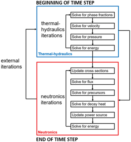
Following a segregated approach, at each time step, the solver first addresses the thermal-hydraulic problem, solving balance equations for mass, momentum, and energy for the phase fractions, velocity, pressure, and temperature fields. Then, the neutronics module is called, determining the neutron flux and the precursor distribution. External iterations are then performed until convergence.

As it can be noticed from Fig. 2, the coupling between the thermal-hydraulic and the neutronics modules is due to several terms:

1. The thermal-hydraulic module provides the void fraction, temperature, and density fields, which influence cross sections. Moreover, the velocity field advects neutron precursors.

2. The neutronics module returns the power density, which heavily affects all other fields. Notice that the power density is itself the sum of two contributions: a prompt one, due to the neutron flux, and the decay heat of FPs.

Fig. 2. Coupling scheme used by the solver.

In the following, a short description of the single-physics solver is presented. The reader is referred to the original publications^[12,13] for all details not reported here.

III.A. Neutronics

The neutronics subsolver can either solve the time-dependent problem or determine the multiplication factor $k_{\mathit{eff}}$ through a power iteration based on the k-eigenvalue formulation of the neutronic problem. For the energy discretization, a multigroup approach is adopted, while for the angular treatment, the user can select either diffusion theory^[13] or the $\mathrm{S}{\mathrm{P}}_3$ approximation.^[17] The former is adopted in this work for the sake of computational time. Albedo boundary conditions are applied to consider the impact on the neutronics of blanket and reflectors that are not explicitly modeled. Energy groups and albedo coefficients are reported in Table II, while groups constants were generated with the Serpent-2 code,^[18] employing cross sections from the JEFF-3.1.1 libraries.^[19] Proper balance equations are adopted for the neutron and decay heat precursors considering eight and three groups, respectively.

TABLE II Employed Energy Groups and Relative Coefficients for Albedo Boundary Conditions

Group	Energy MeV)	Reflector Albedo Coefficient	Blanket Albedo Coefficient
1	$2.23\mathrm{to}20.00$	$0.1455$	$0.1249$
2	$4.98\times {10}^{-1}\mathrm{to}2.23$	$0.5440$	$0.3849$
3	$2.48\times {10}^{-2}\mathrm{to}4.98\times {10}^{-1}$	$0.7771$	$0.6745$
4	$5.53\times {10}^{-3}\mathrm{to}2.48\times {10}^{-2}$	$0.7206$	$0.7596$
5	$7.49\times {10}^{-4}\mathrm{to}5.53\times {10}^{-3}$	$0.9602$	$0.8475$
6	$0\mathrm{to}7.49\times {10}^{-4}$	$1.3336$	$1.0951$

The neutronics part of the solver, both in diffusion and in $\mathrm{S}{\mathrm{P}}_3$ mode, was verified against a Monte Carlo calculation in Refs. [6] and [17]. The chosen geometry for the multiphysics solver is identical with our two-dimensional (2D) one, discussed below, while in the Monte Carlo analysis, blanket and reflector are explicitly modeled.

III.B. Thermal Hydraulics

From a thermal-hydraulic point of view, the main issue with the description of the bubbling system is the correct representation of the multiphase system represented by the liquid molten salt and the helium gaseous phase. Since interfaces between phases are not fixed, an Euler-Euler approach is employed.^[20] The solver includes, for each phase, the mass, momentum, and energy balance equations plus the ones related to the volume fractions representing the occupation of each phase in the space discretization. Because of the averaging process performed in the Euler-Euler formulation, closure equations for the momentum and energy transfer among different phases are required. Explicit terms are included in the balance equations, considering empirical modeling and correlations for drag, lift, turbulent dispersion, and virtual mass forces. Such an approach, as implemented in the preexisting twoPhaseEulerFoam solver, has been validated for a bubbly flow in Ref. [21].

The modeling choices made in this work are retrieved from Ref. [6]:

1. Virtual mass forces, i.e., the contribution due to incompenetrability of two fluids with nonzero relative acceleration, are modeled through a constant coefficient, $C_{\mathit{VM}}=0.5$.

2. For drag, we use the Schiller-Naumann correlation,^[22]

   (1) $C_D=\left\{\begin{array}{c}\frac{{\displaystyle 24\left(1+0.15{\mathrm{R}\mathrm{e}}_b^{0.687}\right)}}{{\displaystyle \mathrm{R}{\mathrm{e}}_b}}\mathrm{if}\mathrm{R}{\mathrm{e}}_b<1000\\ 44\mathrm{if}\mathrm{R}{\mathrm{e}}_b\ge 1000\end{array}\right.,$(1)

where $\mathrm{R}{\mathrm{e}}_b$ is the bubble Reynolds number, i.e., the Reynolds number referred to the bubble diameter.

• 4. Lift is not considered, based on the assumption that bubbles are so small that the effect of vorticity on momentum transfer between the two phases is negligible.

• 5. Turbulent dispersion is neglected.

• 6. For heat transfer, we employ the Ranz-Marshall correlation,^[23]

(2) $\mathrm{Nu}=2+0.6\cdot {\mathrm{R}\mathrm{e}}_b^{1/2}\mathrm{P}{\mathrm{r}}^{1/3}.$(2)

The bubble diameter $d_b$, necessary for the evaluation of $\mathrm{R}{\mathrm{e}}_b$, is modeled through an isothermal power law,

(3) $d_b=d_0{\left(\frac{p_0}{\mathit{p}}\right)}^{1/3}.$(3)

The reference diameter and pressure $d_0$ and $p_0$ adopted in this work are 3 mm and 1 atm, respectively.

The above choices are thoroughly discussed in Ref. [24], where a sensitivity analysis for each of the above items is performed, one item at a time. The effect of each parameter for bubble transport is quantified through its effect on the void coefficient. The bubble diameter turned out to be the most relevant parameter while correlations for virtual mass forces, drag, and heat transfer have a minor impact.

A standard Reynolds-averaged Navier-Stokes approach is employed to deal with turbulence, using a Lahey $\mathit{k}-\mathit{ϵ}$ model.^[25] Wall treatment is done through standard wall functions. A preliminary sensitivity analysis to the turbulence model can be found in Ref. [24]. In particular, the above model is compared with a Wilcox $\mathit{k}-\mathit{\omega }$ approach. The void coefficient is found to differ in the two approaches by no more than 2.4%. According to the outcomes of Ref. [24], its dependence on the core-averaged void fraction seems similar, suggesting that the bubble in-core distribution does not strongly depend on the turbulence model.

III.C. Gaseous FP Modeling

To properly consider the effect of the helium stream injected in the core on the GFPs, a model for the production, consumption, transport, mass exchange, and removal of the various species is required. In Ref. [8], a multicomponent approach was chosen to explicitly consider ¹³⁵Xe as the species, i.e., component, in the liquid (molten salt) or gaseous (helium) phase. Xenon was selected as the representative GFP for two main reasons: (1) The presence of experimental data coming from the MSRE are of paramount importance in calibrating the models and (2) ¹³⁵Xe was the most important species in the MSRE due to its neutron poisoning effect. On the other hand, in the MSFR, which is a fast reactor, this cannot be taken for granted, and an extension to deal with multiple species has been performed to have a more comprehensive analysis. In the following, we briefly summarize the extended modeling for multiple GFPs and the selection of the most relevant GFPs in the MSFR.

III.C.1. Governing Equations

In general, letting $C_{\mathit{k},\mathit{i}}$ denote the concentration of species i in phase k, the mass conservation equation reads

(4) $\frac{\mathrm{\partial }}{\mathrm{\partial t}}\left({\alpha }_k{C}_{\mathit{k},\mathit{i}}\right)+\mathrm{\nabla }\cdot \left({\alpha }_k{\mathit{u}}_k{C}_{\mathit{k},\mathit{i}}\right)-\mathrm{\nabla }\cdot \left({\alpha }_k{D}_{\mathit{k},\mathit{i}}\mathrm{\nabla }{C}_{\mathit{k},\mathit{i}}\right)={\dot{m}}_{\mathit{k},\mathit{i}}+S_{\mathit{k},\mathit{i}}.$(4)

A diffusion approach within each phase is used, with diffusion coefficient $D_{\mathit{k},\mathit{i}}$ for the transport of species i inside phase k. The main modeling issue is to represent the net mass transfer term ${\dot{m}}_{\mathit{k},\mathit{i}}$ for species i toward phase $\mathit{k}$. The term $S_{\mathit{k},\mathit{i}}$ is a source (or sink) term for species i in phase k.

Before proceeding, we rewrite the diffusion coefficients $D_{\mathit{k},\mathit{i}}$ in terms of the Schmidt number,

(5) $\mathrm{S}{\mathrm{c}}_{\mathit{k},\mathit{i}}=\frac{{\nu }_k}{D_{\mathit{k},\mathit{i}}}.$(5)

The mass transfer term can now be modeled as

(6) ${\dot{m}}_{\mathit{k},\mathit{i}}=K_{\mathit{k},\mathit{i}}{a}_{\mathit{k},\mathit{k}{\mathit{ }}^{\mathrm{\prime }}}\left(C_{k,i}^{\ast }-C_{\mathit{k},\mathit{i}}\right)$(6)

with an appropriate coefficient $K_{\mathit{k},\mathit{i}}$. Here, $K_{\mathit{k},\mathit{i}}$ denotes the phase from which species i arrives, and $C_{k,i}^{\ast }$ is the saturation concentration of species i at the interface. For simplicity, here we are assuming contact between at most two phases, which is true in our case. The term $a_{\mathit{k},\mathit{k}{\mathit{ }}^{\mathrm{\prime }}}$ is the interfacial exchange area per unit volume. For the case in which we are interested, a gas g bubble in liquid l, it can be found from the bubble diameter $d_b$ as

(7) $a_{\mathit{g},\mathit{l}}=6\frac{{\alpha }_g}{d_b},$(7)

with ${\alpha }_g$ the phase fraction of the gas.

We still need some expression for the coefficients $K_{\mathit{k},\mathit{i}}$ and for the saturation concentrations $C_{k,i}^{\ast }$. Given the approach used, this requires some experiment-based correlation. For this reason, we employ results obtained from the MSRE activity, as selected in Ref. [8].

First, the interface saturation composition is expressed in terms of the concentration on the other side of the interface through Henry’s law, i.e.,

(8) $C_{k,i}^{\ast }=\mathit{H}{C}_{\mathit{k}{\mathit{ }}^{\mathrm{\prime }},\mathit{i}}.$(8)

A value for the dimensionless coefficient H in the Xe case is provided in Ref. [26], namely, $\mathit{H}=2.08\times {10}^{-4}.$

As for the coefficient $K_{\mathit{k},\mathit{i}}$, we move to the dimensionless Sherwood number,

(9) $\mathrm{Sh}=\frac{{\mathit{K}}_{\mathit{k},\mathit{i}}{d}_b}{D_{\mathit{k},\mathit{i}}},$(9)

i.e., the ratio between convective and diffusive mass transfer. In this specific case, we employ the Higbie correlation for the Sherwood number,^[27]

(10) $\mathrm{Sh}=1.13\cdot {\mathrm{R}\mathrm{e}}_b^{1/2}\mathrm{S}{\mathrm{c}}^{1/2}.$(10)

The characteristic length and velocity to be used here for the evaluation of the bubble Reynolds number $\mathrm{R}{\mathrm{e}}_b$ are the bubble diameter $d_b$ and the relative velocity between the two phases, with velocities evaluated far from the interface.

The use of the Higbie correlation should be considered preliminary since it was developed for the free-rise of bubbles in a vertical channel, a situation only partially resembling the MSFR condition. In addition, it refers to a laminar flow, whereas the MSFR is obviously turbulent and it is untested for chloride systems. Yet, Eq. (10)(10) $\mathrm{Sh}=1.13\cdot {\mathrm{R}\mathrm{e}}_b^{1/2}\mathrm{S}{\mathrm{c}}^{1/2}.$(10) is the correlation adopted in analyses of ¹³⁵Xe removal at the MSRE, for instance, the Oak Ridge National Laboratory (ORNL) report.^[28] Therefore, and despite the dissimilarities between the MSFR and the MSRE, in the absence of new experimental data, we still adopt 10 as the only correlation having received some sort of validation in MSFR-relevant conditions. Notice, however, that our implementation makes it simple to change the correlation for Sh, so that our solver will be readily adapted if and when new results become available.

The actual implementation of the aforementioned model in OpenFOAM is based on the dimensionless (kg/kg) species concentration:

(11) $Y_{\mathit{k},\mathit{i}}=\frac{{\mathit{C}}_{\mathit{k},\mathit{i}}}{{\rho }_k}.$(11)

This choice leads to the following equation for the species i in phase k:

(12) $\begin{array}{rl}& \frac{\mathrm{\partial }}{\mathrm{\partial t}}\left({\alpha }_k{\rho }_k{Y}_{\mathit{k},\mathit{i}}\right)+\mathrm{\nabla }\cdot \left({\alpha }_k{\rho }_k{u}_k{Y}_{\mathit{k},\mathit{i}}\right)-\mathrm{\nabla }\cdot \left(\frac{{\alpha }_k{\mu }_k}{\mathrm{S}{\mathrm{c}}_{\mathrm{k}}}\mathrm{\nabla }{Y}_{\mathit{k},\mathit{i}}\right)\\ & ={\dot{m}}_{\mathit{k},\mathit{i}}+S_{\mathit{k},\mathit{i}}.\end{array}$(12)

We only have to add appropriate source and sink terms to the above equation, modeling production by fission and destruction via radioactive decay or neutron absorption.

Since fissile material is present only in the liquid phase, the source term will be present only there, and we have

(13) $\mathit{Sourc}{e}_i=\sum _j{\mathrm{\Sigma }}_{\mathit{f},\mathit{j}}{\varphi }_j{y}_i\frac{M_i}{N_a},$(13)

where $M_i$ = molar mass of species i; $N_a$ = Avogadro number. The sum is extended over all energy groups, and $y_i$ is the cumulative fission yield of species i. This corresponds to neglecting short-lived FPs decaying to isotope i.

About the sink term, we have

(14) $\mathit{Sin}{k}_{\mathit{k},\mathit{i}}=-{\alpha }_k{\rho }_k\left({\lambda }_i+\sum _j{\sigma }_{\mathit{a},\mathit{j}}{\varphi }_j\right)Y_{\mathit{k},\mathit{i}}.$(14)

Thus, the final form of the equations in our solver is, denoting with l and g liquid and gas phases, respectively,

(15) $\begin{array}{rl}& \frac{\mathrm{\partial }}{\mathrm{\partial t}}\left({\alpha }_l{\rho }_l{Y}_{\mathit{l},\mathit{i}}\right)+\mathrm{\nabla }\cdot \left({\alpha }_l{\rho }_l{\mathit{u}}_l{Y}_{\mathit{l},\mathit{i}}\right)-\mathrm{\nabla }\cdot \left(\frac{{\alpha }_l{\mu }_l}{\mathrm{S}{\mathrm{c}}_{\mathrm{l}}}\mathrm{\nabla }{Y}_{\mathit{l},\mathit{i}}\right)={\dot{m}}_{\mathit{l},\mathit{i}}+\\ & \sum _j{\mathrm{\Sigma }}_{\mathit{f},\mathit{j}}{\varphi }_j{y}_i\frac{M_i}{N_a}-{\alpha }_l{\rho }_l\left({\lambda }_i+\sum _j{\sigma }_{\mathit{a},\mathit{j}}{\varphi }_j\right)Y_{\mathit{l},\mathit{i}}\end{array}$(15)

and

(16) $\begin{array}{rl}& \frac{\mathrm{\partial }}{\mathrm{\partial t}}\left({\alpha }_g{\rho }_g{Y}_{\mathit{g},\mathit{i}}\right)+\mathrm{\nabla }\cdot \left({\alpha }_g{\rho }_g{u}_g{Y}_{\mathit{g},\mathit{i}}\right)-\mathrm{\nabla }\cdot \left(\frac{{\alpha }_g{\mu }_g}{\mathrm{S}{\mathrm{c}}_{\mathrm{g}}}\mathrm{\nabla }{Y}_{\mathit{g},\mathit{i}}\right)\\ & ={\dot{m}}_{\mathit{g},\mathit{i}}-{\alpha }_g{\rho }_g{\lambda }_i{Y}_{\mathit{g},\mathit{i}},\end{array}$(16)

where we neglect production via neutron absorption or decay of other isotopes, as well as the absorption term in the gas phase.

The above solver was verified, in the one-GFP case, against an analytical benchmark in Ref. [8]. Excellent agreement was found in both single- and two-phase conditions and with different choices of boundary conditions. In particular, the worst mean relative error, 1.5%, was found for Dirichlet conditions in two-phase, while for Neumann single-phase conditions, the error is just 0.002%. Such good values suggest the correct implementation of the mass transfer model. Given as detailed below that we employ the same mass transfer model for all species, this verification remains fully valid for the extended solver.

The current solver thus allows the simulation of an arbitrary number of GFPs. Apart from their nuclear properties, i.e., name, molar mass, decay constant, cumulative yield, and cross sections, information about mass transfer is required in terms of a correlation for the Sherwood number and a value for the Henry coefficient.

III.C.2. GFP Selection

Considering that we are interested in analyzing the effect of the bubbling system in terms of removal of neutron poisons, all different isotopes, even if of a same chemical element, are regarded as different species.

We initially consider noble gases Kr and Xe since these are the ones identified as most important in Refs. [29] and [30], where a burnup Monte Carlo calculation of a MSFR-like system was carried out. More specifically, we consider

1. ⁸⁰Kr, ⁸²Kr, ⁸³Kr, ⁸⁴Kr, ⁸⁵Kr, ⁸⁶Kr.

2. ¹²⁸Xe, ¹²⁹Xe, ¹³⁰Xe, ¹³¹Xe, ¹³²Xe, ¹³³Xe, ¹³⁴Xe, ¹³⁵Xe, ¹³⁶Xe.

Other isotopes of these elements have too-low fission yields or cross sections to contribute appreciably.

To optimize the number of simulated isotopes, we consider their (cumulative) fission yield y, reported in Table III. These values were found with the Monte Carlo code SERPENT-2 and are referred to a neutron energy of $400\mathrm{keV}$.

TABLE III Fission Yields at $400\mathrm{keV}$ for the Investigated Isotopes

Isotope	Fission Yield	Isotope	Fission Yield
^80Kr	$4.801\times {10}^{-8}$	^130Xe	$1.614\times {10}^{-7}$
^82Kr	$8.767\times {10}^{-7}$	^131Xe	$2.306\times {10}^{-2}$
^83Kr	$9.919\times {10}^{-3}$	^132Xe	$2.985\times {10}^{-2}$
^84Kr	$4.639\times {10}^{-2}$	^133Xe	$4.116\times {10}^{-2}$
^85Kr	$9.243\times {10}^{-3}$	^134Xe	$5.883\times {10}^{-2}$
^86Kr	$6.912\times {10}^{-2}$	^135Xe	$5.195\times {10}^{-2}$
^128Xe	$1.346\times {10}^{-6}$	^136Xe	$6.686\times {10}^{-2}$
^129Xe	$6.973\times {10}^{-9}$

From these values, we discard all isotopes having fission yield lower than 10⁻². This leaves us with isotopes ⁸⁴Kr, ⁸⁶Kr, ¹³¹Xe, ¹³²Xe, ¹³³Xe, ¹³⁴Xe, ¹³⁵Xe, and ¹³⁶Xe. We mention that work related to Ref. [29] and based on Monte Carlo simulations shows that these isotopes dominate concentration by several orders of magnitude after 5 years of operation without any form of removal. Of this selection, ⁸⁴Kr and ⁸⁶Kr have cross sections a few orders of magnitude lower than the others, and so, we discard them. Assuming that Kr and Xe have a similar mass transfer, we find that the contribution by Kr isotopes is negligible compared with Xe.

Our final solver includes only Xe isotopes as GFPs. More specifically, we have

1. ¹³¹Xe, stable.

2. ¹³²Xe, stable.

3. ¹³³Xe, radioactive.

4. ¹³⁴Xe, stable.

5. ¹³⁵Xe, radioactive.

6. ¹³⁶Xe, stable.

Notice that of these isotopes, only ¹³³Xe and ¹³⁵Xe are radioactive, with decay constants given by Table IV. Thus, only these two isotopes will contribute to the activity of the removed helium gas.

TABLE IV Decay Constants for Radioactive GFPs

Isotope	Decay Constant (s^–1)
^133Xe	$1.530\times {10}^{-6}$
^135Xe	$2.107\times {10}^{-5}$

Also notice that our mass transfer model was adopted at the ORNL specifically for ¹³⁵Xe. Nevertheless, we expect a very weak isotopic dependence of the model, for the only way different isotopes can be transported in different ways is via their different mass. In all cases, the mass variation of the various isotopes with respect to ¹³⁵Xe is within $\pm 3\mathrm{\%}$. Finally, in our code we assume that isotopes undergoing neutron capture disappear. In particular, we do not include in our equations terms due to neutron absorption of other GFPs.

IV. BUBBLING SYSTEM ANALYSIS AND SIMULATION

In this section, we will employ the multiphysics solver described in Sec. III to analyze some operational and safety-related features of the helium bubbling system.

IV.A. Geometry

We employ two different geometries for our simulations: a two-dimensional (2D) geometry and a three-dimensional (3D) geometry. Unless explicitly specified, all our results refer to the 2D geometry.

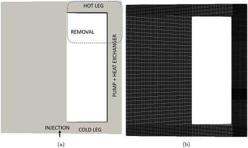
The simplified 2D geometry for the MSFR consists in a cylinder hosting the salt plus the blanket, which is arranged in a rectangular torus inside the cylinder allowing for an axial-symmetric description. A sketch of the employed geometry is in Fig. 3a. The mesh, containing 22 671 cells, is presented in Fig. 3b. Both geometry and mesh have already been employed in several studies as part of the EVOL,^[31] SAMOFAR (https://samofar.eu/), and SAMOSAFER (https://samosafer.eu/) projects. A free surface at the top of the hot leg is present to allow for thermal expansion of the salt. This is important given that the multiphysics solver includes compressibility effects. The region on the right of the blanket also includes the pump and heat exchanger. However, these components are not modeled explicitly but simply via the addition of source or sink terms in the equations for thermal hydraulics. Bubble injection occurs at the cold leg while bubble removal is performed at the hot leg. Again, the components responsible for these operations are modeled via source and sink terms in the balance equations. This geometry is essentially the one initially considered in the EVOL project,^[31] the choice of a cylinder being motivated by neutron economy reasons. However, the presence of sharp edges produces a stagnation region near the inner surface of the blanket.^[32] This negative feature is the reason for moving to the smoother toroidal geometry currently considered for the MSFR.

Fig. 3. (a) Geometry and (b) computational mesh employed for 2D simulations.

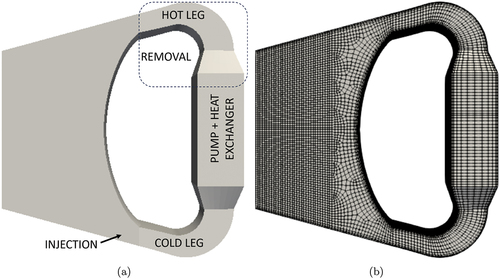
The 3D geometry is depicted in Fig. 4a. It represents 1/16 of the real reactor. The geometry models one of the reactor loops, together with the associated portion of the core. As before, the blanket is arranged in a torus and is not explicitly simulated. Similarly, pump and heat exchanger are modeled through appropriate terms in the momentum and energy equations. With respect to the geometries employed in Refs. [6] and [8], the present one adopts joints in the heat exchange region, thus eliminating the sharp edges present in the aforementioned works. The mesh has 118 550 cells and is represented in Fig. 4b. Despite our not performing a proper sensitivity analysis, we have adopted the mesh relaxing the one adopted in Refs. [8] and [24], which was based on a sensitivity analysis and reached a mesh convergence.^[24]

Fig. 4. (a) Geometry and (b) computational mesh employed for 3D simulations.

The results obtained with the coarse mesh are consistent with the one obtained with the finer mesh, mainly in terms of void coefficient as a function of the void fraction (see Sec. IV.C.1) and cycle time (see Sec. IV.B.1). The comparison of the steady-state distribution of the temperature and fission rate (see Sec. IV.B, Figs. 6b and 6d, respectively) leads to a discrepancy lower than 1% and around 3% for the two quantities, respectively, that could be justified with the slightly different geometry adopted. These evidences support the use of the chosen mesh for this work that should be intended to highlight some qualitative trends rather than a thorough quantitative analysis.

IV.B. Analysis of the Operational Features of the In-Core FP Removal System

The analysis of the operational features of the helium bubbling system concerns four parts:

1. Evaluating the efficiency of GFP removal, through a characteristic removal time.

2. Quantifying the effectiveness of GFP removal, in terms of the poisoning contribution of the removed GFPs.

3. Assessing the activity and decay heat of the removed gas, of crucial importance for the off-gas unit.

4. Calculating the fuel mass flow rate versus power curve to assess the impact of the gaseous phase.

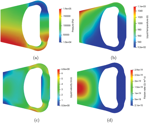
As initial conditions, we employ the main fields found with a stationary simulation in the absence of helium injection. Significant quantities are plotted in Figs. 5 and 6 for the 2D and 3D geometries, respectively. Starting from these conditions, bubbles are injected from the bottom, at the cold leg, and extracted from the top, at the hot leg. During their flow, they extract GFPs from the salt through mass transfer, effectively removing them from the core.

Fig. 5. Initial conditions for quantities of interest: (a) pressure, (b) temperature, (c) velocity, and (d) fission rate with the 2D geometry.

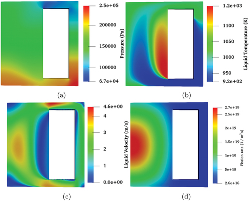
Fig. 6. Initial conditions for quantities of interest: (a) pressure, (b) temperature, (c) velocity, and (d) fission rate with the 3D geometry.

As the initial condition for the GFPs, the values in Tables V and VI are adopted. Since both radioactive and nonradioactive isotopes are present, the choice of the initial inventory for the transient is not trivial. These values are obtained through a steady-state calculation stopped when equilibrium is reached for the radioactive isotope with longest mean life, ¹³³Xe.

TABLE V Initial Inventories for the Various GFPs in 2D Simulations

Isotope	Initial Condition (kg)
^131Xe	$7.60\times {10}^{-3}$
^132Xe	$1.31\times {10}^{-2}$
^133Xe	$8.01\times {10}^{-3}$
^134Xe	$2.99\times {10}^{-2}$
^135Xe	$7.62\times {10}^{-4}$
^136Xe	$3.11\times {10}^{-2}$

TABLE VI Initial Inventories for the Various GFPs in 3D Simulations

Isotope	Initial Condition (kg)
^131Xe	$3.71\times {10}^{-2}$
^132Xe	$6.03\times {10}^{-2}$
^133Xe	$3.69\times {10}^{-2}$
^134Xe	$1.45\times {10}^{-1}$
^135Xe	$3.45\times {10}^{-3}$
^136Xe	$1.50\times {10}^{-1}$

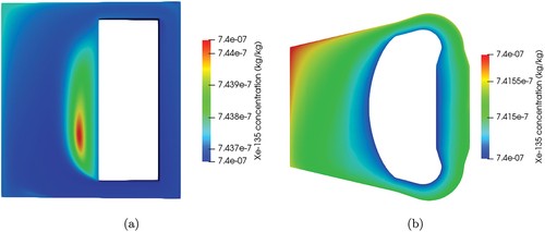
In Fig. 7, the initial concentration of one of the isotopes, ¹³⁵Xe, in both two and three dimensions is plotted. The other isotopes have different values, as discussed above, but their spatial distribution is extremely similar. Notice the absence, in the 3D geometry, of the recirculation region near the edge of the blanket present in the 2D geometry. This is due to the rounder wall profile in the 3D geometry, and it reflects the stagnation region, which is known to characterize the 2D squared geometry.

Fig. 7. Initial distribution of the ¹³⁵Xe isotope in (a) 2D geometry and (b) 3D geometry.

IV.B.1. Evaluation of the Cycle Time

As already mentioned, some previous studies modeled the effect of the bubbling system on the GFP concentration as an additional decay^[7]; i.e., the global inventory of GFPs was assumed to satisfy an equation of the form

(17) $\frac{\mathit{dN}}{\mathit{dt}}=\mathit{Source}-\mathit{Consumption}-\mathit{\lambda N}-{\gamma }_b\mathit{N},$(17)

where $\mathit{\lambda }$ is responsible for radioactive decay and ${\gamma }_b$ intends to model the effect of the helium bubbling system.

In addition to the usefulness of such an assumption in calculations not dealing explicitly with thermal hydraulics, e.g., burnup calculations, ${\gamma }_b$ and its reciprocal, i.e., the cycle time $\mathit{\tau }$,

(18) $\mathit{\tau }=\frac{1}{{\gamma }_b},$(18)

are also useful indicators of the efficiency of the bubbling system.

From Eq. (17)(17) $\frac{\mathit{dN}}{\mathit{dt}}=\mathit{Source}-\mathit{Consumption}-\mathit{\lambda N}-{\gamma }_b\mathit{N},$(17) , assuming that consumption reactions are negligible, as is indeed the case for our isotopes, we need

(19) ${\gamma }_b\gg \mathit{\lambda }$(19)

in order for the bubbling system to be effective. This consideration led to the adoption of the value $\mathit{\tau }=30\mathrm{s}$ in previous works.^[7]

Part of our aim is to evaluate this characteristic time as a function of the bubble flow rate. This was already done in Ref. [8], whose calculation strategy is adopted in this work. At the same time, in addition to what has been done in Ref. [8], some analysis for lower values of bubble flow rate will be performed.

The value ${\gamma }_b$ can be evaluated at each time step as the ratio between the mass flow rate of ¹³⁵Xe leaving the core and the mass of ¹³⁵Xe present in the whole core:

(20) ${\gamma }_b=\frac{\mathrm{X}{\mathrm{e}}_{\mathit{out}}}{\mathrm{X}{\mathrm{e}}_{\mathit{tot}}},$(20)

where the total mass of ¹³⁵Xe present in the core $\mathrm{X}{\mathrm{e}}_{\mathit{tot}}$ is found by direct integration of the concentration over the whole domain. The outwards mass flow rate $\mathrm{X}{\mathrm{e}}_{\mathit{out}}$, instead, is evaluated through a mass balance as

(21) $\dot{\mathrm{X}}{\mathrm{e}}_{\mathit{out}}\left(\mathit{t}\right)=-\frac{\mathrm{X}{\mathrm{e}}_{\mathit{tot}}\left(\mathit{t}\right)-\mathrm{X}{\mathrm{e}}_{\mathit{tot}}\left(\mathit{t}-\mathrm{\Delta t}\right)}{\mathrm{\Delta t}}+S_{\mathit{Xe}}\left(\mathit{t}\right),$(21)

where $S_{\mathrm{Xe}}$ is the mass of ¹³⁵Xe produced by reactions in the whole core. With respect to Eq. (17)(17) $\frac{\mathit{dN}}{\mathit{dt}}=\mathit{Source}-\mathit{Consumption}-\mathit{\lambda N}-{\gamma }_b\mathit{N},$(17) , we are here neglecting both consumption reactions and radioactive decay.

Following this approach, applied to the global GFP inventory identified in Sec. III.C.2 instead of ¹³⁵Xe alone, we find the cycle time $\mathit{\tau }$ for various values of helium flow rate. The results are reported as functions of time in Fig. 8a for the 2D geometry. Some comments can be drawn:

1. After an initial transient, $\mathit{\tau }$ approaches a constant value. This means that apart from an initial transient, during which the void distribution inside the core has yet to stabilize, the assumption of an exponential decay in the GFP population works well.

2. The value $\mathit{\tau }$ is smaller the higher the helium flow rate. This is intuitive and means that the helium bubbling system is more efficient for higher helium flow rates. More specifically, Fig. 8b shows an inverse proportionality between $\mathit{\tau }$ and the helium flow rate.

3. The values of $\mathit{\tau }$ found in this way are consistently smaller than the ones obtained considering ¹³⁵Xe alone, as reported in Ref. [8].

Fig. 8. Efficiency in 2D geometry: (a) time evolution of the cycle time $\mathit{\tau }$ at various helium flow rates and (b) illustration of the inverse proportionality between the cycle time $\mathit{\tau }$ and the helium flow rate. The coefficient of determination R² is 0.994 at 20 s and 0.992 at 30 s.

To understand the reason for which increasing the number of simulated Xe isotopes leads to smaller values of $\mathit{\tau }$, it is necessary to recall from the previous section that our model implies, with the notation used before,

(22) ${\dot{m}}_{\mathit{k},\mathit{i}}\propto \left(C_{k,i}^{\ast }-C_{\mathit{k},\mathit{i}}\right).$(22)

On the other hand, the saturation concentration $C_{k,i}^{\ast }$ is modeled through Henry’s law, so

(23) $C_{k,i}^{\ast }\propto C_{\mathit{k}{\mathit{ }}^{\mathrm{\prime }},\mathit{i}},$(23)

where $\mathit{k}{ }^{\mathrm{\prime }}$ is the phase on the other side of the interface. Letting k be the gas and $\mathit{k}{ }^{\mathrm{\prime }}$ the salt, we see that increasing the concentration of GFPs in the salt increases the saturation concentration. Since new helium is continuously injected into the core, the concentration in the gas does not increase in the same way, and so, by Eq. (22)(22) ${\dot{m}}_{\mathit{k},\mathit{i}}\propto \left(C_{k,i}^{\ast }-C_{\mathit{k},\mathit{i}}\right).$(22) , mass transfer increases.

In Figs. 9a and 9b, the cycle time and the inverse proportionality between $\mathit{\tau }$ and the helium flow rate are shown for the 3D geometry.

Fig. 9. Efficiency in 3D geometry: (a) time evolution of the cycle time $\mathit{\tau }$ at various helium flow rates and (b) illustration of the inverse proportionality between the cycle time $\mathit{\tau }$ and the helium flow rate. The coefficient of determination R² is 0.988.

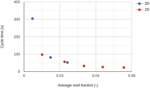
The comparison between the 2D and 3D results (summarized in Table VII) is interesting to assess possible 3D effects. In order to compare the results, we should rescale the helium fraction and the helium mass flow rate in the axial-symmetric and the 1/16 geometry to be compliant with each other in terms of average helium fraction in the active zone for the mass exchange. The cycle times for both geometries are provided against the average helium fraction in the mass exchange zone in Table VIII. The results highlight the direct dependence of the average helium fraction on the cycle time making the 2D and 3D geometries fully compatible once the average helium fraction is the same, as can be seen from Fig. 10. Clearly, the latter is influenced by the geometry of the case and the location of the helium injection and removal.

TABLE VII Comparison Among Cycle Times Found in Two Dimensions and Three Dimensions*

Two Dimensions		Three Dimensions
Helium Flow Rate (g/s)	Cycle Time (s)	Helium Flow Rate (g/s)	Cycle Time (s)
0.1	97	0.1	304
0.2	56	0.3	81
0.3	32	0.5	52
0.4	26
0.5	23

*Helium flow rates refer here to the values in the simulation.

TABLE VIII Comparison Among Cycle Times Found in Two Dimensions and Three Dimensions Against the Average Helium Fraction*

Average Helium Fraction	Cycle Time (s)	Simulation
0.0047	304	3D – 0.1 g/s
0.0101	97	2D – 0.1 g/s
0.0148	81	3D – 0.3 g/s
0.0226	56	2D – 0.2 g/s
0.0242	52	3D – 0.5 g/s
0.0334	32	2D – 0.3 g/s
0.0439	26	2D – 0.4 g/s
0.0556	23	2D – 0.5 g/s

*The values in the simulation column refer to the geometry and helium flow rate used in the calculation.

Fig. 10. Graphical representation of the data reported in Table VIII.

IV.B.2. GFP Neutron Poisoning

Even if in the MSFR the function of the helium bubbling system in removing the neutron poison is less important than in a thermal reactor, it is still relevant to evaluate its capability to avoid the buildup of GFPs that can impact the neutron economy. This is even more important considering that in its present design, the MSFR does not foresee any control rod for reactivity adjustment.

To evaluate the GFP poisoning term, we follow two different strategies:

1. We perform single-phase eigenvalue calculations to determine the effective multiplication factor $k_{\mathit{eff}}$ of the system in the absence of helium and with all GFPs present. Then, we repeat the calculation removing the GFP term from the neutronics equation. The difference in $k_{\mathit{eff}}$ is ascribed to the poisoning effect of GFPs.

2. We calculate the variation in $k_{\mathit{eff}}$ from the beginning to the end of the GFP removal transient. This is done deactivating cross-section updating, so that thermal feedback does not contribute. Then, the value for the void coefficient we find in the next section is employed to separate the variation of $k_{\mathit{eff}}$ into a void and a GFP poisoning contribution.

These two strategies provide essentially identical values for the reactivity contribution of GFPs. Numerically, we have, in absolute value, 38 pcm. Performing the same procedure with only ¹³⁵Xe gives a contribution of only 0.1 pcm.

The value we found, 38 pcm, should be compared with both the circulating delayed fraction ${\beta }_{\mathit{circ}}$ and with the reactivity inserted by the change in void fraction. In particular, this reactivity is not negligible in absolute terms, corresponding to roughly $0.3\mathrm{\$}$.

IV.B.3. Activity and Decay Heat

Designing the helium bubbling system and the off-gas unit clearly requires information about the activity of the removed gas. This would determine which kind of radioprotection devices are useful and, via decay heat, whether a dedicated cooling circuit is required for the tank. Considering the GFPs selected in Sec. III.C.2, focusing on the radioactive ones, and setting as initial conditions the ones provided in Sec. IV.B, i.e., the situation of a couple of weeks without any removal, we find the activity and decay heat stated in Table IX. These values are referred to the entire core, even if they are calculated with the 3D geometry representing 1/16 of the system. Two-dimensional calculation provides very similar values.

TABLE IX Contributions to Activity and Decay Heat of the Removed Gas Found with the 3D Geometry*

Isotope	Activity (Bq)	Decay Heat (W)
^133Xe	$8.85\times {10}^{17}$	$2.55\times {10}^4$
^135Xe	$1.14\times {10}^{18}$	$1.03\times {10}^5$
Total	$2.03\times {10}^{18}$	$1.28\times {10}^5$

*Values are referred to the whole core.

We can see that values for the decay heat are in the range of hundreds of kilowatts. This is a value that can pose some concern in terms of rejection of this amount of heat, also considering that our analysis completely ignores metallic FPs, which should also be removed by the bubbling system. The previous figures represent an underestimation of the real decay heat that needs to be removed in the off-gas system unit to avoid reaching temperatures that could be detrimental for the system structure.

We also report in Fig. 11 the activity rate leaving the core during the removal transient. This is obviously extremely dependent on the adopted removal strategy and on the initial conditions. Our result is for a couple of weeks without any removal, and it shows again that the GFP removal transient, apart from the very beginning, during which the bubble distribution has yet to stabilize, is very well described as exponential.

Fig. 11. Activity leaving the core in the gas per unit time found with the 3D geometry, referred to the whole core. Notice the logarithmic scale.

IV.B.4. Fuel Mass Flow Rate Versus Power Curve

Finally, we consider the power variation following a change in fuel salt flow rate. The knowledge of the power versus flow rate curve is of crucial importance if the mass flow rates in the three circuits are used in the reactor control strategy, as some proposals suggest.^[9]

It is not immediate what the effect of a flow rate variation would be. Indeed, we have two contrasting mechanisms:

1. A variation in precursor motion, which tends to decrease power as flow rate increases.

2. A variation in void fraction, which tends to increase power as flow rate increases.

Before proceeding to the actual result, we obtain a curve for the circulating delayed fraction ${\beta }_{\mathit{circ}}$. Starting from stationary single-phase conditions, we simulate variations in the salt mass flow rate. This is done with neutronics in eigenvalue mode and deactivating all feedback mechanisms apart from precursor motion. By acting appropriately on delayed fraction and neutron spectrum, we are able to find values for the circulating delayed fractions ${\beta }_{\mathit{circ}}$. The result is in Fig. 12.

Fig. 12. Circulating delayed fraction as a function of flow rate.

We see that ${\beta }_{\mathit{circ}}$ stays roughly constant, at a value of about 130 pcm, for flow rate variations of $\pm 40\mathrm{\%}$ from nominal conditions. In particular, the associated reactivity variation only becomes comparable with characteristic thermal or void feedback for flow rates below 20% of the nominal flow rate, i.e., an accidental condition.

Our results can be compared with those obtained in Ref. [33] through a variety of means, including analytical calculations, multiphysics simulations similar to ours, and Monte Carlo simulations. The general trend is similar to the one of Fig. 12 presented in Ref. [33] despite the latter referring to a ²³⁵U-started system instead of a ²³³U-started one as in the present work. For the ²³³U-started system, the delayed neutron fraction calculated in Ref. [33] lays between $124\pm 3$ and $146\pm 3\mathrm{pcm}$ for the nominal flow rate depending on the sampling strategy, in full agreement with the 130 pcm calculated in this paper.

We can now simulate variations in salt flow rate in the two-phase system, obtaining Fig. 13. We can see that power increases as flow rate increases. This is an indication that void fraction variation dominates over precursor motion. The behavior depicted in Fig. 13 is the opposite of what occurs in single-phase conditions and is a clear indication that the void fraction strongly affects the fuel mass flow rate versus power curve. Notice that the helium flow rate is here our reference value of 0.1 g/s in the 2D geometry, i.e., about 0.3 g/s per core sector in the actual reactor, which is not regarded as a high value.

Fig. 13. Power variation, void fraction, and salt temperature as functions of flow rate variation.

IV.C. Safety-Related Analysis

The presence of an in-core bubbling system poses some questions from a safety point of view. If on one hand the benefit of the GFPs is remarkable, on the other hand this system introduces a gaseous phase in the core that, given the negative void coefficient of the MSFR, impacts mainly the neutronics of the system.^[6] Any possible initiator events related to the helium bubbling system are based on the variation of the void fraction in the core. As a first step, we evaluate the void coefficient introduced in the system with the multiphysics solver and compare it with previously obtained values. Then, two possible accidents will be evaluated: (1) loss of helium injection and (2) loss of helium removal.

IV.C.1. Void Coefficient

The void coefficient is calculated for different helium flow rates using the eigenvalue mode of the solver and comparing the situation with and without a developed helium stream in the core. The results are presented in Table X for the 2D geometry. These values can be compared with those found in Ref. [6], which investigates void fractions comparable to the Table X first row. The agreement is within 10%.

TABLE X Void Coefficient at Various Helium Flow Rates in 2D Geometry

Helium Flow Rate (g/s)	Void Fraction (%)	Void Coefficient ($\mathrm{pcm}/\mathrm{\%}$)
0.1	0.69	$-293$
0.2	1.8	$-245$
0.3	3.2	$-218$
0.4	5.0	$-192$
0.5	6.9	$-187$

It is clear that the Table X values correspond to reactivities that exceed ${\beta }_{\mathit{circ}}$. Thus, prompt supercriticality may occur at these values of helium flow rate in case the helium gas immediately disappears from the core. If this is the case, the limit of 0.3 g/s of helium per reactor circulation loop should apply when we rescale our results to the whole reactor. On the other hand, the hypothesis of an immediate disappearance of the gaseous phase is unrealistic. In order to consider also the dynamics of the thermal hydraulics, in Secs. IV.C.2 and IV.C.3, we analyze two possible initiator transients with the multiphysics solver.

IV.C.2. Loss of Helium Injection Accident

We first consider loss of helium injection. We assume that at 0 s, starting from stationary two-phase conditions, helium injection is completely stopped. No countermeasure is taken, and helium removal continues to work as usual. Stationary two-phase conditions refer here to a helium flow rate of 0.1 g/s in the 2D geometry.

In Fig. 14, we plot the evolution of power, void fraction, and mean salt temperature. We see that power attains a maximum at about $+75\mathrm{\%}$ with respect to the nominal conditions and then decreases, stabilizing at about $+40\mathrm{\%}$. A qualitative explanation can be drawn as follows. Since helium is no longer being injected but is being removed, the void fraction in the core drops as the gas present in the system is transported toward the removal region. Then, the reduction in void fraction injects positive reactivity, increasing power that in turn increases the core temperature, inducing thermal feedback that stabilizes the power level.

Fig. 14. Normalized power, void fraction, and mean salt temperature after losing helium injection.

Despite the fact that the initial void fraction would have led to a prompt supercriticality if the helium had disappeared immediately, the dynamics of the transient from a thermal-hydraulic point of view grants a “slow” evolution of the transient, allowing the reactivity temperature feedback to intervene.

IV.C.3. Loss of Helium Removal Accident

As for the loss of helium removal, we assume that at 0s, starting from stationary two-phase conditions, helium removal is completely stopped. No countermeasure is taken, and helium injection continues to work as usual.

With respect to the previous case, we can anticipate that equilibrium will not be reached. Since helium injection is assumed to continue, the void fraction will keep increasing until the complete shutting down of the reactor. Therefore, we simulate just the first 10s of this transient.

In Fig. 15, we plot the time behavior of both power and void fraction. As expected, void fraction increases linearly with time. Correspondingly, power decreases. However, we also notice that there is a delay in power reduction. This can be explained as a geometrical effect due to helium removal occurring mainly in the hot leg. When loss of removal occurs, the helium that was about to be removed is advected by the salt into the steam generator. Being outside of the core, helium in the steam generator does not contribute to reactivity. After being transported to the cold leg, helium is reinjected into the core, thus contributing to reactivity and generating a delay between loss of helium removal and power reduction that is due to helium flowing out-of-core. This is confirmed by Fig. 16, where the void fraction is plotted at the beginning of the transient and after 10s.

Fig. 15. Normalized power and void fraction after losing helium removal.

Fig. 16. Volume fraction of the gas at the beginning (left) and after 10s (right) of loss of helium removal. Notice the common scale.

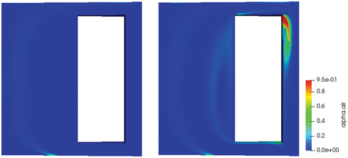
It is worth noting that such an accident, despite leading to a shutdown without any external intervention, is not entirely harmless. In fact, as Fig. 16 shows, the amount of gas in the pump region will greatly increase in a relatively short time. This will most likely damage the pump.

V. CONCLUSIONS

This work presents a comprehensive analysis of the possible use of an in-core bubbling system for FP removal to be employed in the MSFR. Our analysis is based on a multiphysics solver in order to assess different aspects from both the neutronics and the thermal-hydraulic points of view. The previous tool has been extended in order to deal with multiple GFP species given the lack of a predominant nuclide of interest like the ¹³⁵Xe in a thermal reactor.

The solver is employed in the analysis of the helium bubbling system, both for its operational characterization and for safety-related studies. Since removal efficiency is the first characteristic for the in-core bubbling system, this is modeled through a characteristic cycle time, for which we provide values at various helium mass flow rates. Typical values are in the range of several tens of seconds and agree with previous estimates. The dependence of the cycle time on the average helium fraction is found to be very similar in 2D and 3D simulations, indicating that simplified 2D geometries can be used to describe GFP production, transport, and removal once the average helium fraction has been established.

The poisoning effect of GFPs in the Xe family, after prolonged operation without any kind of removal, amounts to tens of pcm. In this light, the only isotope considered in previous works, ¹³⁵Xe, turns out to be negligible. Since the stable isotopes are not in equilibrium in these conditions, in the absence of removal, their poisoning contribution will continue to increase with time.

Another aspect of importance for the design not only of the bubbling system but also of the off-gas unit is the activity and decay heat of the removed gas. The calculated values, which correspond to letting radioactive isotopes reach equilibrium in-core and then starting removal, range in the hundreds of kilowatts, indicating the need of a dedicated cooling system for the off-gas unit.

Also of importance for the characterization of the in-core bubbling system is its impact on the fuel salt flow rate–power curve. This aspect is relevant for the control features of the MSFR considering the absence of control rods for load-following adjustment. A possible choice is to employ mass flow rates in the different circuits. Our results show that in the absence of the bubbling system, an increase of salt flow rate causes power to decrease due to precursor motion, but the opposite occurs when a helium stream is present in the core, due to variation in the void fraction.

The analysis performed in this work aims also at qualitatively assessing the trade-off between the removal requirements and the safety feature of the reactor. The presence of a void fraction in the core may cause a reactivity-initiated accident in case of stop of the helium injection. An upper limit of 0.3 g/s per core sector on the helium flow rate is found in order to avoid prompt supercriticality in case of sudden disappearance of the gaseous phase. On the other hand, a more realistic investigation has been performed analyzing the transient evolution of a loss of helium injection, showing that the MSFR thermal-hydraulic behavior tends to avoid prompt supercriticality even in case the reactivity associated with the void feedback exceeds the delayed fraction. A less concerning transient is the loss of helium removal, which has no consequences on safety but could be problematic for the accumulation of gas in the reactor.

It is worthwhile to remind that our results account for the contribution of gaseous FPs only, neglecting the contribution of the metallic ones. In addition, the outcomes are dependent both on the geometry and on the location of bubble injection and removal. In this view, further analyses could help the design of this system by investigating the best location for injection and removal. In addition, different models and correlations for mass transfer could be tested and investigated if experimental results are made available. Finally, a further extension of the solver to model also metallic FPs could provide a complete analysis of the in-core helium bubbling system of the MSFR.

Disclosure Statement

No potential conflict of interest was reported by the author(s).

Data Availability Statement

The data that support the findings of this study are openly available in Zenodo at http://doi.org/10.5281/zenodo.7515490.

Additional information

Funding

This project has received funding from the Euratom research and training programme 2014–2018 under grant agreement number 847527.

References

- M. TIBERGA et al., “Preliminary Investigation on the Melting Behavior of a Freeze-Valve for the Molten Salt Fast Reactor,” Ann. Nucl. Energy, 132, 544 (2019); http://dx.doi.org/10.1016/j.anucene.2019.06.039.
- B. R. BETZLER et al., “Modeling and Simulation Functional Needs for Molten Salt Reactor Licensing,” Nucl. Eng. Des., 355, 110308 (2019); http://dx.doi.org/10.1016/j.nucengdes.2019.110308.
- S. DELPECH et al., “Reactor Physic and Reprocessing Scheme for Innovative Molten Salt Reactor System,” J. Fluorine Chem., 130, 1, 11 (2009); http://dx.doi.org/10.1016/j.jfluchem.2008.07.009.
- H. B. ANDREWS et al., “Review of Molten Salt Reactor Off-Gas Management Considerations,” Nucl. Eng. Des., 385, 111529 (2021); https://doi.org/10.1016/j.nucengdes.2021.111529.
- Z. TAYLOR et al., “Implementation of Two-Phase Gas Transport into VERA for Molten Salt Reactor Analysis,” Ann. Nucl. Energy, 165, 108672 (2022); http://dx.doi.org/10.1016/j.anucene.2021.108672.
- E. CERVI et al., “Multiphysics Analysis of the MSFR Helium Bubbling System: A Comparison Between Neutron Diffusion, SP3 Neutron Transport and Monte Carlo Approaches,” Ann. Nucl. Energy, 132, 227 (2019); http://dx.doi.org/10.1016/j.anucene.2019.04.029.
- M. AUFIERO et al., “An Extended Version of the SERPENT-2 Code to Investigate Fuel Burn-Up and Core Material Evolution of the Molten Salt Fast Reactor,” J. Nucl. Mater., 441, 1, 473 (2013); https://doi.org/10.1016/j.jnucmat.2013.06.026.
- F. CARUGGI et al., “Multiphysics Modelling of Gaseous Fission Products in the Molten Salt Fast Reactor,” Nucl. Eng. Des., 392, 111762 (2022); http://dx.doi.org/10.1016/j.nucengdes.2022.111762.
- C. TRIPODO, S. LORENZI, and A. CAMMI, “Definition of Model-Based Control Strategies for the Molten Salt Fast Reactor Nuclear Power Plant,” Nucl. Eng. Des., 373, 111015 (2021); http://dx.doi.org/10.1016/j.nucengdes.2020.111015.
- A. CAMMI et al., “Transfer Function Modeling of Zero-Power Dynamics of Circulating Fuel Reactors,” J. Eng. Gas Turbines Power, 133, 5 (2010); http://dx.doi.org/10.1115/1.4002880.
- C. FIORINA et al., “Modelling and Analysis of the MSFR Transient Behaviour,” Ann. Nucl. Energy, 64, 485 (2014); http://dx.doi.org/10.1016/j.anucene.2013.08.003.
- E. CERVI et al., “An Euler-Euler Multiphysics Solver for the Analysis of the Helium Bubbling System in the MSFR,” Proc. 26th Int. Conf. Nuclear Energy for New Europe (NENE 2017), Bled, Slovenia, September 11–14, 2017, p. 202.1, Nuclear Society of Slovenia (2017).
- E. CERVI et al., “Development of a Multiphysics Model for the Study of Fuel Compressibility Effects in the Molten Salt Fast Reactor,” Chem. Eng. Sci., 193, 379 (2019); http://dx.doi.org/10.1016/j.ces.2018.09.025.
- H. WELLER et al., “A Tensorial Approach to Computational Continuum Mechanics Using Object Orientated Techniques,” Comput. Phys., 12, 620 (1998); http://dx.doi.org/10.1063/1.168744.
- J. SERP et al., “The Molten Salt Reactor (MSR) in Generation IV: Overview and Perspectives,” Prog. Nucl. Energy, 77, 308 (2014); http://dx.doi.org/10.1016/j.pnucene.2014.02.014.
- M. ALLIBERT et al. “7 – Molten Salt Fast Reactors,” Handbook of Generation IV Nuclear Reactors, Woodhead Publishing Series in Energy, p. 157, I. L. PIORO, Ed., Woodhead Publishing; https://doi.org/10.1016/B978-0-08-100149-3.00007-0.
- E. CERVI et al., “Development of an SP3 Neutron Transport Solver for the Analysis of the Molten Salt Fast Reactor,” Nucl. Eng. Des., 346, 209 (2019); http://dx.doi.org/10.1016/j.nucengdes.2019.03.001.
- J. LEPPÄNEN et al., “The Serpent Monte Carlo Code: Status, Development and Applications in 2013,” Ann. Nucl. Energy, 82, 142 (2015); http://dx.doi.org/10.1016/j.anucene.2014.08.024.
- A. SANTAMARINA et al., “The JEFF-3.1.1 Nuclear Data Library. Validation Results from JEF-2.2 to JEFF-3.1.1,” OECD 2009 NEA No. 6807, Organisation for Economic Co-operation and Development, Nuclear Energy Agency (2009).
- H. RUSCHE, “Computational Fluid Dynamics of Dispersed Two-Phase Flows at High Phase Fractions,” PhD Thesis, Imperial College London, University of London (2002).
- A. GHIONE, “Development and Validation of a Two-Phase CFD Model Using OpenFOAM,” Master’s Thesis, Royal Institute of Technology (2012).
- L. SCHILLER and A. NAUMANN, “Über die grundlegenden Berechnungen bei der Schwerkraftaufbereitung,” Z. Ver. Dtscher. Ing., 77, 12, 318 (1933).
- W. E. RANZ and W. R. MARSHALL, “Evaporation from Drops. Parts I & II,” Chem. Eng. Prog., 48, 142 (1952).
- E. CERVI, “An Innovative Multiphysics Modelling Approach for the Analysis and the Development of the Generation IV Molten Salt Fast Reactor,” PhD Thesis, Politecnico di Milano (2020).
- R. T. LAHEY, “The Simulation of Multidimensional Multiphase Flows,” Nucl. Eng. Des., 235, 10, 1043 (2005); https://doi.org/10.1016/j.nucengdes.2005.02.020.
- R. KEDL and A. HOUTZEEL, “Development of a Model for Computing 135Xe Migration in the MSRE,” Oak Ridge National Laboratory (1967).
- R. HIGBIE, “The Rate of Absorption of a Pure Gas into a Still Liquid During Short Periods of Exposure,” Trans. AIChE, 31, 365 (1935).
- F. PEEBLES, “Removal of Xenon-135 from Circulating Fuel Salt of the MSBR by Mass Transfer to Helium Bubbles,” Oak Ridge National Laboratory (1968).
- G. MERLA, “Improvement of Continuous Reprocessing and Fuel Composition Adjustment Capabilities in SERPENT-2 for Molten Salt Reactors,” Master’s Thesis, Politecnico di Milano (2021).
- G. MERLA, A. CAMMI, and S. LORENZI, “A New Reactivity Control Approach for Circulating Fuel Reactors,” Proc. 30th Int. Conf. Nuclear Energy for New Europe, Bled, Slovenia, September 6–9. 2021, p. 206.1, Nuclear Society of Slovenia (2021).
- B. BROVCHENKO et al., “Optimization of the Pre-Conceptual Design of the MSFR,” EVOL Project (2013).
- M. AUFIERO et al., “Development of an OpenFOAM Model for the Molten Salt Fast Reactor Transient Analysis,” Chem. Eng. Sci., 111, 390 (2014); http://dx.doi.org/10.1016/j.ces.2014.03.003.
- E. M. AUFIERO et al., “Calculating the Effective Delayed Neutron Fraction in the Molten Salt Fast Reactor: Analytical, Deterministic and Monte Carlo Approaches,” Ann. Nucl. Energy, 65, 78 (2014); http://dx.doi.org/10.1016/j.anucene.2013.10.015.