A distributional approach to measuring lifespan stratification

Abstract

The study of the mortality differences between groups has traditionally focused on metrics that describe average levels of mortality, for example life expectancy and standardized mortality rates. Additional insights can be gained by using statistical distance metrics to examine differences in lifespan distributions between groups. Here, we use a distance metric, the non-overlap index, to capture the sociological concept of stratification, which emphasizes the emergence of unique, hierarchically layered social strata. We show an application using Finnish registration data that cover the entire population over the period from 1996 to 2017. The results indicate that lifespan stratification and life-expectancy differences between income groups both increased substantially from 1996 to 2008; subsequently, life-expectancy differences declined, whereas stratification stagnated for men and increased for women. We conclude that the non-overlap index uncovers a unique domain of inequalities in mortality and helps to capture important between-group differences that conventional approaches miss.

Keywords:

• mortality inequality
• measurement
• life expectancy
• lifespan inequality
• income
• Finland

Introduction

Mortality reduction and longevity extension are progressing unequally at the global, regional, national, and subnational levels. In 2018, life expectancy at birth was 63 years among low-income countries, 18 years lower than in high-income countries (World Bank 2021). Numerous studies have documented that even within high-income countries, differences in life expectancy between socio-economic groups can be strikingly large. In the United States (US), for instance, men in the top 1 per cent of the income distribution lived 14.6 years longer on average than those in the bottom 1 per cent during the period 2001–14 (Chetty et al. 2016). Large gaps in life expectancy between socio-economic groups have been reported in many other countries and at different times (e.g. Brønnum-Hansen and Baadsgaard 2012; Martikainen et al. 2014; Mackenbach et al. 2018).

The reduction of mortality inequalities arguably constitutes one of the major public health challenges and is important for further advances in human longevity as a whole. To date, a large segment of the literature examining between-group differences in longevity has focused on the comparison of group averages, such as age-standardized mortality rates and life expectancies. While life expectancy is undoubtedly a powerful mortality indicator, other important facets of between-group differences in longevity can be hidden if life expectancy alone is studied.

To better the understanding of between-group differences in longevity, we introduce and quantify a new concept: lifespan stratification. Measuring lifespan stratification belongs to an approach that has been taken less frequently—comparing the distance and non-overlap between lifespan distributions—and which is conceptually different from conventional approaches of comparing central tendencies (e.g. life expectancy) or variabilities. We show that the non-overlap index we use operationalizes the long-standing sociological concept of social stratification and reveals the extent to which society is divided into unique social strata when individual longevity is the outcome variable. Our empirical example of lifespan stratification between Finnish income groups illustrates that this new measure reveals new inequality patterns. Hence, our measure is a useful addition to the demographer’s toolbox of analysis on mortality differences.

Conventional approaches to measuring mortality differences

Measurement of differences in lifespan distributions between population subgroups has generally been approached in one of the following ways: (1) by comparing measures of central tendency (e.g. mean, median, mode); (2) by comparing the spread or prematureness of mortality (e.g. variability, years of life lost (YLL)); or (3) by comparing overall distributions using statistical distance measures (e.g. Kullback–Leibler divergence (KLD)). Here we review the first two approaches, before focusing on statistical distance measures in the next section.

Comparing central tendencies

Earlier work on social differences in mortality has tended to compare age-standardized mortality rates between social groups using rate ratios (Whitney 1934; Logan 1954; Kitagawa and Hauser 1973; Duleep 1989). Rate ratios show the relative difference between groups, while rate differences show the actual size of the inequality. Life expectancy has also long been used by prior studies to examine group differences in mortality (Antonovsky 1967; Brønnum-Hansen and Baadsgaard 2012; Chetty et al. 2016). It is the mean value of the lifespan distribution from the life table, and a comparison of life expectancies can be used to indicate the average number of years by which a group of individuals outlives another group. Other measures of central tendency, such as the modal and median age at death, have long been included in mortality analysis and have enriched demographers’ understanding of the evolution of human longevity (Lexis 1878; Kannisto 2001; Cheung and Robine 2007; Canudas-Romo 2008, 2010; Ouellette and Bourbeau 2011; Cohen and Oppenheim 2012; Horiuchi et al. 2013). Recent research on mortality differences between population subgroups has started to incorporate these additional central tendency measures beyond the traditional comparisons of life expectancy (Brown et al. 2012; Zarulli et al. 2012; Diaconu et al. 2022).

Like mortality rates, central tendency measures can also be compared using ratios or differences. In practice, life expectancy ratios are less frequently reported than life-expectancy differences. Absolute and relative measures yield the same patterns of inequalities when population subgroups are examined at a given time, when the aim is to understand whether group A is performing better than group B. However, absolute and relative measures may contradict each other when the goal is to examine how the magnitude of mortality difference between A and B varies across time or place: for example, when seeing whether the sex difference in life expectancy is larger in one country than in another. Adding a dimension of time or place to social differences in mortality complicates the comparison of central tendency measures. For illustration, we compare life expectancies at birth for men in three countries. In 2018, life expectancies for men in Nigeria, Pakistan, and Hong Kong were 53, 66, and 82 years, respectively (World Bank 2021). Consider two comparisons: (1) difference in life expectancy between Nigeria and Pakistan; and (2) difference in life expectancy between Pakistan and Hong Kong. The mean difference between Pakistan and Nigeria was 13 years and between Hong Kong and Pakistan was 16 years, suggesting that mortality difference was larger between Hong Kong and Pakistan than between Pakistan and Nigeria. However, life expectancy for men in Pakistan was 1.25 times that of Nigeria, while life expectancy for men in Hong Kong was 1.24 times that of Pakistan, suggesting that mortality difference was more similar between Hong Kong and Pakistan than between Pakistan and Nigeria. Therefore, monitoring life expectancy inequalities using differences and ratios can yield inconsistent results. Similarly, slope and relative indices of inequality when examined on mortality rates often lead to different conclusions about the direction of changes in inequalities (e.g. Mackenbach et al. 2018).

In summary, assessing whether the longevity gap has been growing or diminishing and whether policies have been successfully narrowing the gap can depend on whether absolute or relative measures are used (Carter-Pokras and Baquet 2002; Harper and Lynch 2017). The potential inconsistency in the two types of measures is perhaps a limitation of this approach.

Comparing variabilities

A recent strand of research has shifted the attention from group differences in means to group differences in variabilities (Edwards and Tuljarpukar 2005; Brown et al. 2012; Permanyer et al. 2018; van Raalte et al. 2018). Lifespan variability measures the within-group heterogeneity in ages at death. It also captures the degree of lifetime uncertainty that a random individual from that group faces. For individuals, lower uncertainty conditional on the same expected lifespan means greater security, which, as economists have argued, people would rather gain at the expense of losing a few years of expected life (Edwards 2013). A wide range of variability measures are available, due to the well-researched area of income inequality. Lifespan variability measures include the interquartile range, Gini coefficient, coefficient of variation, and standard deviation. In demography, metrics such as the life table entropy (H) and life disparity (e†) have been introduced due to their useful interpretations (Leser 1955; Keyfitz 1977; Goldman and Lord 1986; Vaupel 1986; Vaupel and Canudas-Romo 2003).

The theory of mortality compression predicts that as mortality reduction continues, lifespans tend to be concentrated around the mean age at death and thus the survival curve evolves towards a more rectangular shape (Fries 1980; Myers and Manton 1984). Indeed, research has shown that rising life expectancy was historically often coupled with falling lifespan variability (Smits and Monden 2009; Vaupel et al. 2011). Cross-sectional data have shown that lower socio-economic groups tend to exhibit larger lifespan variability in addition to lower life expectancy (Edwards and Tuljarpukar 2005; van Raalte et al. 2011; Brown et al. 2012). These findings point to the so-called ‘double burden’ (van Raalte et al. 2018) among people of lower socio-economic status (SES); that is, compared with high-SES individuals, low-SES individuals not only live shorter lives on average but also face greater uncertainty about the timing of death.

The theoretical prediction and the empirical associations between life expectancy and lifespan variability seem to challenge the motivation for including lifespan variability in research on between-group differences in mortality. However, recent evidence has suggested that for some populations or population subgroups (e.g. lower-SES individuals), increasing life expectancy has been associated with stagnating or increasing lifespan variability (Brønnum-Hansen 2017; Aburto and van Raalte 2018; Permanyer et al. 2018; van Raalte et al. 2018). Hence, comparing lifespan variability between social groups is helpful for detecting additional dimensions of inequalities.

Comparing distributions

Unlike the approaches of comparing central tendency measures and lifespan variabilities, our approach takes into account differences in the whole range of lifespan distributions (i.e. by measuring statistical distance).

Statistical distance

How big is the difference between two lifespan distributions? This question relates to the concept of statistical distance. Measures of statistical distance can quantify the distance between two populations or two probability distributions, and they capture how much ‘effort’ is needed to transform one lifespan distribution into another. Statistical distance measures have been widely used in many disciplines, including biology, chemistry, information theory, mathematics, mechanical engineering, and statistics (Cha 2007).

All distance metrics need to fulfil four conditions (Deza and Deza 2009). Consider a distance metric $D(A,B)$ where A and B are two distributions. The four conditions are expressed as follows:

1. $D(A,B)\ge 0$ (non-negativity);

2. $D(A,B)=0$, if and only if A and B are identical (identity of indiscernibility);

3. $D(A,B)=D(B,A)$ (symmetry);

4. $D(A,B)+D(B,C)\ge D(A,C)$ (triangle inequality).

A related concept to statistical distance is divergence, based on the idea of entropy that originated in information theory (Shannon 1948). Unlike distance metrics, divergence need satisfy only conditions (1) and (2), although the term divergence is sometimes used interchangeably with statistical distance (Ullah 1996). A well-known divergence measure is the KLD (Kullback and Leibler 1951).

The distributional approach using measures of distance and divergence offers new research opportunities for the analysis of mortality differences, beyond summary measures such as mean, mode, and variance. Numerous distance and divergence measures (see an overview in Cha 2007) can be used to answer the question of how big the difference between two lifespan distributions is. Thus far, only a few studies have taken this distributional approach. Sasson (2016) used the KLD to examine the divergence in age-at-death distributions between educational groups. (Note that throughout this paper, ‘age-at-death distribution’ refers to the life table dx, rather than the observed deaths, Dx.) Edwards and Tuljapurkar (2005) and d’Albis et al. (2014) also used the KLD to compare country-specific lifespan distributions. As a divergence measure, the KLD does not satisfy the symmetry and triangle inequality conditions.

Conceptualizing stratification

Different distance and divergence measures have unique properties that provide different information. We use a distance metric to quantify the concept of stratification of lifespan. In sociology, stratification is defined as the phenomenon of society being divided into hierarchically layered strata, characterized by historical, cultural, and economic distinctions (Mann 1984). Social class, education, and income are among the most common social stratifiers of a society (Grusky and Weisshaar 2014). The use of terminology in the existing literature is wide-ranging. The stratifier is often inserted before the term ‘stratification’, for example gender in ‘gender stratification’. It is also common use to insert the outcome before ‘stratification’; for instance, ‘income stratification’ has been used in prior research where income is the outcome (e.g. Yitzhaki and Lerman 1991; Allanson 2014; Zhou and Wodtke 2019). In our study, lifespan is the outcome and income is the stratifier. We use the terms ‘lifespan stratification’ and ‘the stratification of lifespan’ interchangeably.

In a broad sense, stratification is often a synonym of inequality, yet Yitzhaki and Lerman (1991) argued that stratification is conceptually different from inequality, the latter often being measured by the distance between group means. Social stratification emphasizes the formation of observable layers based on group characteristics (Lasswell 1965). Put differently, stratification reflects the extent to which social groups form unique strata but does not show how big the differences in group means are. According to this rationale, life-expectancy difference between social groups is a good measure of inequality but is not suitable for measuring stratification. When we discuss stratification, it is strictly this narrower phenomenon of distributional distance that we are referring to. The emphasis of stratification on distinguishable strata and noticeable boundaries coincides partly with the concept of statistical distance. Both stratification and statistical distance relate to the phenomenon of two distributions being distinct.

Prior research using the narrow definition of stratification has focused almost exclusively on outcomes such as income and wealth, and little is known about the stratification of lifespan. Admittedly, unlike income, lifespan cannot be redistributed across individuals. But unequal lifespans arise partly from unequal distributions of both monetary and non-monetary resources (Link and Phelan 1995; Lynch et al. 2000; Marmot 2005; Phelan et al. 2010). Examining the stratification of lifespan can therefore inform us how health-related resources are stratified between social groups and can shed new light on research into mortality differences.

Formalizing stratification

Consistent with prior research on the stratification of income (Zhou and Wodtke 2019), we propose to quantify the stratification of lifespan by the proportion of non-overlap of two lifespan distributions. This measure relates to the Jaccard index, originally used by ecologists to measure similarity in flora between districts (Jaccard 1912), and the Tanimoto index (Tanimoto 1958), a measure widely used in chemical research to quantify molecular similarity. The Jaccard and Tanimoto similarity metrics are mathematically equivalent. They are calculated as the ratio of the intersection to the union, that is, $(A\cap B)/(A\cup B)$ (i.e. overlap/total). The Jaccard (Tanimoto) distance is calculated as $1-Jaccard(Tanimoto)similarity$. For probability distributions, the Jaccard (Tanimoto) distance is also equivalent to the Wave Hedges index (Cha 2007). (We agree with Prasath et al. (2017) that the name ‘Wave Hedges’ is questionable, as the formula for the Wave Hedges index cannot be traced to the original paper by Hedges [1976] as cited in Cha [2007]). Due to the inconsistent naming of this measure, we refer to it as the non-overlap index, with notation $S_{ij}$, for the stratification of lifespan between (sub)populations $i$ and $j$. Note that here $i$ and $j$ can be two subpopulations or any two populations where the comparison is substantively meaningful (e.g. US vs Japan). $S_{ij}$ is calculated as follows: (1) $\begin{array}{c}{S}_{ij}=1-{\displaystyle \frac{{\int }_{\alpha }^{\omega }\min \{d_i(x),d_j(x)\}\mathrm{d}x}{{\int }_{\alpha }^{\omega }\max \{d_i(x),d_j(x)\}\mathrm{d}x}}\end{array}$(1) where $\alpha$ is the starting age, $\omega$ is the maximum lifespan, and $d_i(x)$ and $d_j(x)$ are life table age-at-death distributions for (sub)populations $i$ and $j$, respectively.

$S_{ij}$ reaches the maximum of one when two age-at-death distributions do not overlap (maximum stratification) and the minimum of zero when two distributions are identical (no stratification). Stratification increases monotonically as $S_{ij}$ increases from zero to one. It can easily be proved that this index satisfies the four aforementioned conditions of a distance metric (Kosub 2019). This is an advantage as compared with the asymmetric measure KLD used in earlier research (e.g. Sasson 2016); it is arbitrary whether the KLD between groups A and B is measured from A to B or from B to A. The non-overlap index is not just a distance measure but also captures the sociological concept of stratification, which makes it easier to interpret than other distance measures.

Furthermore, a larger proportion of non-overlapping lifespans means a greater likelihood that a random individual in the group with lower life expectancy will die earlier than another random individual from the group with higher life expectancy. This concept is closely related to the outsurvival probability (Bergeron-Boucher et al. 2020; Vaupel et al. 2021). Stratification and the outsurvival probability both rely on the topological relationship between two lifespan distributions. Yet unlike the outsurvival probability, which focuses interpretations at the individual level, stratification reflects the unequal distributions of lifespans at the societal level.

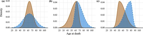
Although the non-overlap index always captures the extent to which two distributions differ from each other, it is not designed as a measure of the tendency for values from one distribution to be higher (or lower) than those from the other. Thus, the non-overlap index is not suitable for measuring lifespan stratification, unless $x$ and $\{d_i(x)-d_j(x)\}/\{d_i(x)+d_j(x)\}$ are strongly correlated. This way, lifespan distributions can be seen as hierarchically layered. Figure 1(a) shows an example where two distributions do not fulfil this condition. However, for human populations, $x$ and $\{d_i(x)-d_j(x)\}/\{d_i(x)+d_j(x)\}$ tend to be strongly correlated, because human populations follow similar patterns of lifespan distribution and because the central tendency and the dispersion of a lifespan distribution are generally negatively correlated, both cross-sectionally and over time. It is worth mentioning that the same value of the non-overlap index may result from scenarios where the skewness and location (age) of the distributions differ. In Figure 1, panels (b) and (c) show the same proportions of non-overlap as each other (around 2/3), but panel (b) displays a situation where the two distributions occupy a wider range of lifespans. In panel (b) no individuals from the shorter-lived group survive to ages above 85, where a big part of the non-overlap from the longer-lived group lies. Consequently, compared with panel (c), the two distributions in panel (b) arguably occupy more unique strata and thus their stratification is higher. In such a case, the non-overlap index would not be an appropriate metric of lifespan stratification. Again, these cases are unlikely to be observed in human populations.

Figure 1 Special cases where the non-overlap index cannot perform well

Source: Authors’ own.

To illustrate the conceptual differences and the possible links between stratification and the two conventional approaches, we show four hypothetical scenarios of the stratification of lifespan in Figure 2(a)–(d). In panels (a) and (b), the life expectancies of the two social groups are 70 (left) and 75 (right); thus, the life-expectancy difference between the two groups is five years. As the two groups in Figure 2(a) exhibit low standard deviations and the two groups in Figure 2(b) show high standard deviations, the stratification levels in the two panels are different, with moderate stratification for panel (a), and low stratification for panel (b). In Figure 2(c) and (d), there is a 10-year difference in life expectancy between the two groups. Panel (c) displays a higher level of lifespan stratification than panel (d) due to its low standard deviations in both groups. If we examine these panels vertically—comparing Figure 2(a) with (c) or Figure 2(b) with (d)—the standard deviations of the two groups are the same, but as life-expectancy differences increase, stratification also increases. Therefore, stratification can be affected by differences in both life expectancy and standard deviation.

Figure 2 Hypothetical scenarios of age-at-death distributions in two groups

Source: As for Figure 1.

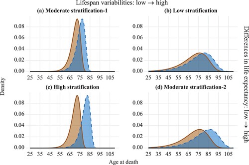
Our stylized examples suggest that the relationships between stratification and the other two types of measure of between-group differences are unclear. The three indicators may respond differently to mortality changes at different locations (ages) in the distributions; thus, over time, they may produce different or even conflicting trends, as has been observed for the stratification of other types of social goods (Zhou and Wodtke 2019). For instance, in the high-stratification scenario depicted in Figure 2(c), individuals in the lower-mortality group all survive to middle age, whereas no one from the higher-mortality group survives to old age. If the oldest people in the lower-mortality group were to live longer, or if those individuals in the higher-mortality group who die at young ages were to die at an even younger age, differences in life expectancy would increase, while stratification would remain invariant.

Unlike the two conventional approaches that comprise both absolute and relative measures, the non-overlap index for the stratification of lifespan is a relative measure and does not have an absolute counterpart. As a non-parametric index, the value of $S_{ij}$ is not dependent on actual lifespan values but on the relative location of the two distributions. A monotonic transformation of the lifespans of all individuals (by adding/subtracting some years or including a scaling factor) will not change the value of $S_{ij}$.

Multigroup stratification

Calculation of the stratification index becomes less straightforward if we are interested in comparing multiple groups. Constructing a stratification index for multiple groups involves several considerations. First, we need to decide whether interest lies in overall stratification or in stratification with regard to a reference group. We propose to measure overall stratification, $S_{Total}$, by a weighted sum of all pairwise comparisons: (2) $\begin{array}{c}{S}_{Total}={\displaystyle \frac{{\sum }_{1\le i<j\le N}^N{w}_i{w}_j{S}_{ij}}{{\sum }_{1\le i<j\le N}^N{w}_i{w}_j}}\end{array}$(2) where N denotes the total number of (sub)populations, and $w_i$ and $w_j$ are the sizes of (sub)populations i and j, respectively (when $i=j$, $S_{ij}=0$). It is essential to include all pairwise comparisons, as the two-group stratification is not transitive, that is, one combination of $S_{AB}$ and $S_{AC}$ can lead to different values of $S_{BC}$. See Figure A1 in the supplementary material for an example.

An alternative is to calculate stratification with regard to a reference group (e.g. the highest SES group or the best-performing group). We propose to measure the reference-based stratification as a weighted sum of all comparisons in which one group is always the reference group, R: (3) $\begin{array}{c}{S}_R={\displaystyle \frac{{\sum }_{1\le i\le N}^N{w}_R{w}_i{S}_{Ri}}{{\sum }_{1\le i\le N}^N{w}_R{w}_i}}\end{array}$(3) where $S_R$ denotes the multigroup stratification with a reference group R, and $w_R$ and $w_i$ are the sizes of (sub)populations R and i, respectively (when $i=R$, $S_{Ri}=0$). The selection of a reference group may involve normative judgments (Harper et al. 2010) and has implications for interpretation. Choosing the best-performing group as the reference group quantifies the extent of mortality inequality that could be eradicated if lifespans of those in the disadvantaged groups could be extended to those enjoyed by the lowest mortality group. Alternatively, we could use the population average as the reference group. This would imply that reducing the lifespan of the longer lived is one way to achieve low stratification. However, this is unlikely to be acceptable, even to egalitarians, and does not recognize that lifespans are not directly transferable.

Lastly, the choice of weights also has consequences for interpretation. Weights based on population size may be considered to reflect the public health relevance of lifespan differences. However, if a socially disadvantaged group comprises a small number of individuals, should we care less about them? We might argue that each group is equally important (Harper and Lynch 2017). Such justification may lead to giving all groups being compared equal weights.

An empirical example of lifespan stratification between income groups in Finland

In this section, we present an empirical example of the stratification of lifespan between Finnish income groups. Finland is used because it benefits from an exceptionally long time series of full population data by income percentile and shows mortality inequalities comparable with countries and regions such as the US and western Europe (Mackenbach et al. 2005; Elo et al. 2006; Mortensen et al. 2016). The results are based on period life tables by sex, year, and income quintile (measured in the year prior to exposure). Only individuals aged 25 and above are included, meaning that all reported measures in the example are conditional on surviving to age 25. From these life tables we calculated the remaining life expectancy (hereafter life expectancy), remaining lifespan variation (hereafter lifespan variation), and stratification indices. See an overview of the data set in the supplementary material (Appendix B).

Lifespan distributions

We first investigate how the age-at-death distributions have evolved differently for those in the lowest and highest income quintiles (20 per cent income groupings). Figure 3 shows the distributions for three periods: 1996–2000, 2006–10, and 2013–17. The vertical lines mark the mean ages at death for the two distributions in each panel. From 1996–2000 to 2013–17, there was a general pattern of mortality moving toward older ages for both women and men regardless of income group, which resulted in increases in life expectancy. However, mortality evolved differently in the lowest and highest income groups at certain ages. For men in the lowest income group, there were early ‘humps’ in the age-at-death distributions across ages 55–70 for 2006–10 and 2013–17. Accordingly, life-expectancy differences between low- and high-income men rose from 9.0 years in 1996–2000 to 12.2 years in 2006–10 and then dropped to 9.8 years in 2013–17. Similarly, stratification increased from 0.42 in 1996–2000 to 0.54 in 2006–10 and then dropped to 0.49 in 2013–17. We find that lifespan-variability differences (measured by standard deviation differences) increased in both 2006–10 and 2013–17.

Figure 3 Lifespan distributions for highest and lowest income quintiles by sex: Finland, 1996–2000, 2006–10, and 2013–17

Notes: Dashed lines show the values of mean age at death. S refers to lifespan stratification; Δe₂₅ refers to the difference in life expectancy at age 25; ΔSD refers to the difference in the standard deviations.

Source: Authors’ own calculations based on Finnish registry data.

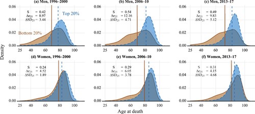
Similar to the findings for men, a less pronounced hump in deaths at around retirement age also emerged for low-income women. From 1996–2000 to 2006–10, the life-expectancy difference increased from 4.5 to 6.1 years, and stratification increased from 0.24 to 0.29. In 2013–17, low-income women caught up with their high-income counterparts in the proportion of deaths occurring at ages above 90. However, a large number of low-income women were still dying at relatively younger ages. It seems that among low-income women, the improvement at older ages more than compensated for the apparent stagnation at younger ages, leading to a counter-intuitive result: life-expectancy difference between the two income groups decreased to 4.2, while stratification increased to 0.31. Similar to the results for men, we find that lifespan-variability differences increased in both 2006–10 and 2013–17.

Trends in life expectancy and lifespan variability by income

How did life expectancy and lifespan variability in Finland evolve for each income group? Before turning to our analysis of lifespan stratification, we investigate the two most commonly used health indicators. Figure 4 presents the trends in life expectancy at age 25 and lifespan variability, by income quintile and sex from 1996 to 2017. As expected, there was a persistent income gradient in life expectancy for both men and women; the differences were larger among men than women. At the beginning of our study, life expectancy for men aged 25 ranged between 43.6 and 51.8 years for different income quintiles, whereas life expectancy for women aged 25 hovered between 53.3 and 57.5 years. Over the years, life expectancy increased for both sexes in all five income groups, with slight fluctuations in certain years. By 2017, life expectancy had risen to 48.2–57.9 years for men and to 57.3–60.9 years for women.

Figure 4 Trends in life expectancy and lifespan variability at age 25, by income quintile and sex: Finland, 1996–2017

Note: e₂₅ refers to life expectancy at age 25; SD₂₅ refers to lifespan variability at age 25, as measured by the standard deviation.

Source: As for Figure 3.

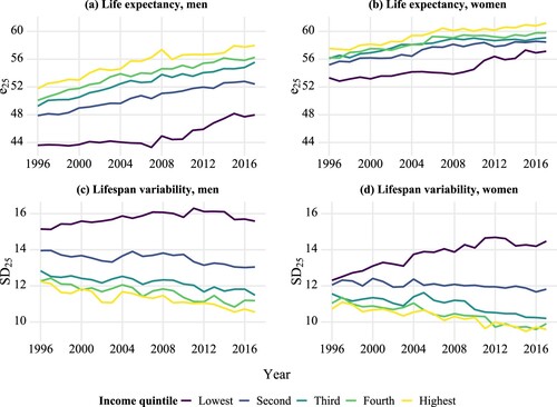
We find that those groups with higher life expectancy tended to display lower lifespan variability. Women showed lower lifespan variability than men, and higher income groups showed lower lifespan variability than lower income groups. However, unlike life expectancy trends, lifespan variability trends diverged across different income groups, especially for women. Lifespan variability decreased for the top four income quintiles, but increased for the lowest quintile.

Trends in lifespan stratification and in life-expectancy and lifespan-variability differences

We proceed by displaying in Figure 5 the trends in lifespan stratification and in the other two measures of differences between the lowest and the highest income quintiles, respectively. The overall lifespan stratification across all five quintile groups shows very similar trends to the one we present here (see Figure A2 in the supplementary material). Figure 5(a) shows that lifespan stratification between the richest and the poorest 20 per cent (for convenience, hereafter referred to as ‘lifespan stratification’) increased from 1996 to 2017 for both men and women. Lifespan stratification among men increased from 0.39 in 1996 to 0.55 in 2007 and then decreased to 0.50 in 2017, while lifespan stratification among women increased by 36 per cent, from 0.24 in 1996 to 0.33 in 2017. In more recent years, stratification continued to increase for women, whereas it decreased slightly for men.

Figure 5 Trends in lifespan stratification and differences in life expectancy and lifespan variability at age 25 between the lowest and highest income quintiles, by sex: Finland, 1996–2017

Note: S refers to lifespan stratification; Δe₂₅ refers to the difference in life expectancy at age 25; ΔSD₂₅ refers to the difference in the standard deviations.

Source: As for Figure 3.

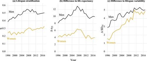
Figure 5(b) indicates that for both men and women, life-expectancy differences increased over the first decade but decreased between 2008 and 2017, and life expectancy ratios generally show the same pattern (see Figure A3 in the supplementary material). The trends for men and women are highly consistent, except that the life-expectancy differences for women fell to a lower level in 2017 (4.0 years) than their initial level in 1996 (4.2 years). For both lifespan stratification and life-expectancy difference, we find that men showed larger values than women. Comparing trends in life-expectancy difference with trends in lifespan stratification, we observe that the two trends were similar for men but also, interestingly, that the trends were different for women in the most recent years: their life-expectancy difference dropped, whereas their lifespan stratification continued to rise.

From Figure 5(c), we find that the absolute differences in lifespan variability increased consistently over the whole period for both men and women. The trends in relative difference in lifespan variability are very similar (see ratios in Figure A4, supplementary material). Yet in contrast to findings in Figure 5(a) and (b), which show that the differences in the indicator remained more or less at the same level for men and women, in Figure 5(c) we see a convergence in lifespan-variability difference for men and women. Whereas lifespan-variability differences were much larger for men than for women in the earlier years, this gap had almost disappeared by 2017, especially for lifespan variability ratios (Figure A4, supplementary material).

To determine how different age groups contributed to the divergent trends we observe, we can either conduct a decomposition analysis or simply inspect the age-at-death distributions at different periods. Looking back at Figure 3, we note that for the low income group, faster mortality improvements at more advanced ages raised life expectancy and compensated for the lack of improvements at younger ages. However, the excessive deaths at pre-retirement ages (the hump) among the low income group increased their lifespan variability as well as the lifespan stratification.

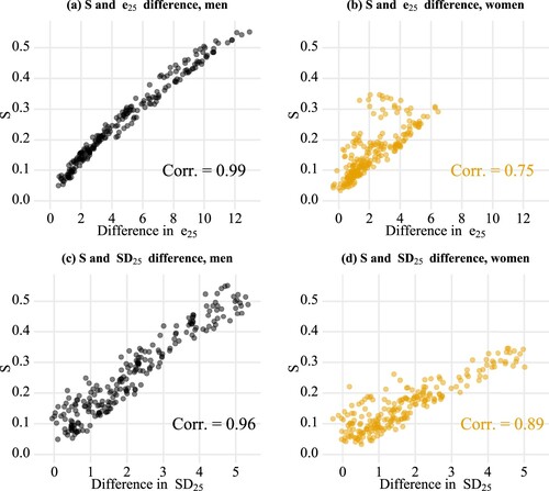
How was lifespan stratification associated with life-expectancy and lifespan-variability differences? Figure 6 shows these associations using all pairwise comparisons between each two income quintiles (for each year, there are 10 different pairs of five income groups for both men and women). Life-expectancy and lifespan-variability differences were strongly associated with lifespan stratification for men; however, the associations were much weaker for women. Put differently, for women, there was a large range in lifespan stratification, given the same levels of life-expectancy or lifespan-variability differences. Among women, lifespan stratification was more closely correlated with the lifespan-variability differences than with life-expectancy differences.

Figure 6 Pairwise associations between lifespan stratification and two other measures—life-expectancy differences and lifespan-variability differences—by sex, Finland, 1996–2017

Notes: Each point refers to a comparison between two income groups (e.g. the lowest and the second lowest income quintile groups, or the third and the highest income quintile groups) in a given year. The colour becomes darker when multiple data points overlap. S refers to lifespan stratification; e₂₅ refers to life expectancy at age 25; SD₂₅ refers to the standard deviation at age 25; Corr. is the Pearson correlation coefficient.

Source: As for Figure 3.

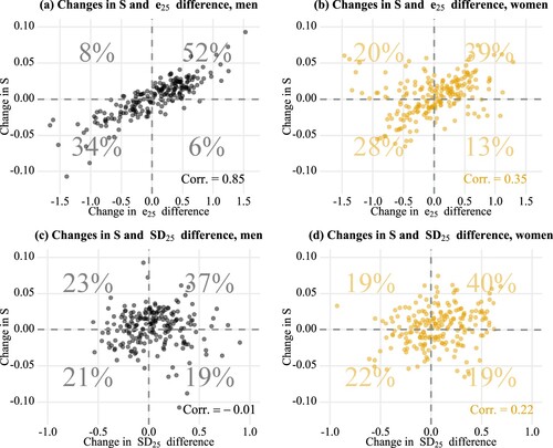
Year-on-year changes

On its own, Figure 6 cannot tell us how the indices were connected to each other over time. An interesting question is whether the direction of change in lifespan stratification was consistent with the direction of change in the life-expectancy or lifespan-variability differences. For this reason, Figure 7 shows the association between yearly changes in stratification and yearly changes in life-expectancy differences (panels (a) and (b)) and lifespan-variability differences (panels (c) and (d)), using all of the pairwise comparisons, as in Figure 6. Panels (a) and (b) show that changes in stratification were more consistent with changes in life-expectancy differences for men (r = 0.85) than for women (r  =  0.35). For men, both these changes simultaneously increased 52 per cent of the time and simultaneously decreased 34 per cent of the time. An increase in stratification coupled with a decrease in life-expectancy differences occurred only 8 per cent of the time (upper-left quadrant) and the other way around just 6 per cent of the time. For women, desirable changes (i.e. decreases in both indicators, lower-left quadrant) occurred 28 per cent of the time, while increases in both indicators occurred 39 per cent of the time. It is notable that around 20 per cent of the time, lifespan stratification increased while life-expectancy differences decreased (upper-left quadrant). Interestingly, changes in lifespan-variability difference (panels (c) and (d)) were not associated with changes in lifespan stratification for men (r  =  −0.01), and the association for women was weak (r  =  0.22).

Figure 7 Pairwise associations between year-on-year changes in lifespan stratification and year-on-year changes in two other measures—life-expectancy differences and lifespan-variability differences—by sex, Finland, 1996–2017

Note: Each point refers to a comparison between two income groups (e.g. the lowest and the second lowest income quintile groups, or the third and the highest income quintile groups) in a given year. The colour becomes darker when multiple data points overlap. S refers to lifespan stratification; e₂₅ refers to life expectancy at age 25; SD₂₅ refers to the standard deviation at age 25; Corr. is the Pearson correlation coefficient.

Source: As for Figure 3.

Discussion

In this paper, we introduced the concept of lifespan stratification and demonstrated how to measure it. The non-overlap index reflects the extent to which individuals’ lifespans are stratified by their social characteristics, and it also captures the distance between two lifespan distributions. Monitoring stratification can uncover between-group differences that go unnoticed in the two conventional approaches—comparing life expectancy or lifespan variability—and can help to link these two lines of research. Our empirical application to Finland showed that income has come to play an increasingly important role in the stratification of lifespan in Finland, while life-expectancy differences have decreased in recent years.

Our contribution is mainly methodological. From a mathematical perspective, the vast majority of research on between-group mortality differences has focused almost exclusively on only two moments of distributions: mean and variance. Measuring distributional differences is conceptually different from comparing central tendency measures or lifespan variabilities. We could argue that because of the strong regularity of the age pattern of mortality, knowing the life-expectancy difference can inform the overall distributional distance. This is only partly true. Given two life expectancies, the range of stratification is relatively predictable. However, how they change over time is much less so. It is possible for distributional distance to diverge when life expectancies converge. This point was clearly illustrated by our empirical examples (see Figure 3(d) and (f), and the upper-left quadrants in Figure 7(a)–(b)). Further, although showing similar trends, lifespan-variability difference is conceptually different from our distributional approach, because comparing lifespan variability does not take the location of the distributions into account. As the distance and stratification depend on the life expectancy and lifespan variability of two distributions, our approach links these two lines of research nicely. Lastly, many regression-based inequality indices, such as the relative index of inequality (Regidor 2004), can only be applied to ordinal independent variables. Thus, our index is of particular use when the stratifier is not ordinal, for example in the case of marital status or region, variables which are of great interest in health inequality research.

Thus far, only a few previous studies have taken the approach of measuring distributional dissimilarity, using the KLD (Edwards and Tuljapurkar 2005; d’Albis et al. 2014; Sasson 2016), which is asymmetric and less easy to interpret. The non-overlap index has several advantages. First, as a distance metric, it has a simple graphical representation and interpretation: the more overlap between two lifespan distributions, the smaller the distance. Second, it reflects the sociological concept of social stratification, which focuses on the process of clear boundaries forming between social strata in a society. The majority of prior stratification research that emphasizes the geometric distance between two distributions has focused on the distributions of economic outcomes (e.g. Yitzhaki and Lerman 1991; Zhou and Wodtke 2019). To date, little is known about how lifespan distributions are stratified.

The non-overlap index for the stratification of lifespan should be included in the toolkit for future analysis of mortality inequality, along with existing metrics, such as differences in life expectancy, lifespan variability, YLL, cross-sectional average length of life (CAL), and other CAL-family measures (Brouard 1986; Guillot 2003; Canudas-Romo and Guillot 2015; Sauerberg et al. 2020; Nepomuceno et al. 2022). This is because we need an array of measures to reflect different dimensions of mortality inequalities. For example, for the low income group in our data, a mid-life mortality hump emerged over the follow-up, while old-age mortality declined and approached that of the high income group. Together these trends resulted in an increasing distance between the two lifespan distributions and was captured by our index. As alcohol-related mortality is prominent at the ages around this mortality hump in the low income group (Tarkiainen et al. 2012), we postulate that changes in alcohol consumption may have played an important role in driving the recent increase in stratification. Diverging health behaviours may be explained by changing access to health-related information and technology or important social networks (Link and Phelan 1995; Glied and Lleras-Muney 2008; Montgomery et al. 2020). With survey data, future work could examine whether these factors correlate with lifespan stratification.

A growing literature has documented widening gaps in life expectancy between socio-economic groups in high-income countries over the last few decades (e.g. Meara et al. 2008; Brønnum-Hansen and Baadsgaard 2012; Tarkiainen et al. 2012; Chetty et al. 2016; Sasson 2016; Permanyer et al. 2018; Sasson and Hayward 2019). Our empirical example showed that for the Finnish population, income-group differences in life expectancy increased over the period 1996–2008 and then decreased during 2008–2017. Yet average lifespans do not tell the whole story. First, stratification increased even during periods in which life-expectancy differences remained stable or decreased, particularly for women. The correlations between yearly changes in lifespan stratification and yearly changes in the other two measures were weak, indicating that life expectancy comparisons did not fully capture the developments in mortality inequalities that occurred during the last decade. Second, although the trends in lifespan-variability differences and stratification were similar for men and women, lifespan-variability differences by income level were approximately the same for men and women in recent years, whereas lifespan stratification was noticeably higher for men than for women. Sex differences in the stratification of lifespan by income were relatively stable over time, a pattern similar to the results for life-expectancy differences. Further decomposition between men and women (Figure A5, supplementary material) showed that temporal mortality changes at older ages accounted for much of the convergence in lifespan-variability differences, whereas they played a much less important role in driving the sex differences in the other two indices.

Previous work has shown that the ages and causes of death that drive differences in population-level life expectancy in high-income countries are not the same as those that drive differences in population-level lifespan variability (Seligman et al. 2016). Lifespan variability is generally more sensitive to mortality change at younger ages than life expectancy (van Raalte and Caswell 2013). In contemporary low-mortality settings, mortality change at young adult ages is particularly important in driving trends in lifespan variability (van Raalte et al. 2014; Aburto et al. 2020), whereas life expectancy trends tend to be driven by mortality change at ages where the death density is higher, that is, older ages (Vaupel 1986; Rau et al. 2018). Yet, little is known about the age patterns that drive trends in mortality disparities between socio-economic groups. We conducted supplementary analyses to disentangle the total change in the three metrics between the lowest and highest income groups from the first to the last of the five-year periods (i.e. the same periods that we showed in Figure 3; results can be found in Figure A6, supplementary material) into age-specific components. These analyses indicated that the age patterns are distinct in the three metrics. The overall age pattern of stratification is more similar to that of life-expectancy differences, but is more concentrated in ages 50–74. Older ages are much more important in driving the trends in lifespan-variability differences than in the other two metrics.

The most prominent causes of death for ages 50–74 are circulatory system diseases and neoplasms (GBD 2016 Causes of Death Collaborators 2017). Alcohol-related causes may also play an important role, especially at pre-retirement ages. Indeed, much of the stagnation in life expectancy in the lowest income quintile during the 2000s and the subsequent increase in 2010s was attributable to changes in alcohol-related mortality at pre-retirement ages (Tarkiainen et al. 2012, 2017). Thus, one policy implication is that efforts should be made to reduce alcohol- and smoking-related deaths among low-income individuals in the middle and early old age groups (Martikainen et al. 2014; Tarkiainen et al. 2012, 2017). Reducing such deaths would not only increase life expectancy and reduce lifespan variability for the low-SES group but would also lead to a declining trend in lifespan stratification. However, the roles of alcohol consumption and smoking in contributing to life-expectancy differences by income vary by country. Their relevance is particularly strong in Finland (Östergren et al. 2019); thus, policies tackling them are particularly called for.

When lifespan is highly stratified in a society, disadvantaged individuals are not only more likely to die earlier, but they also tend to experience more premature deaths among members of their social and kinship networks over their life course (Daw et al. 2016; Umberson et al. 2017). This becomes more important at older ages, when lower-SES individuals have fewer strong ties. Research has shown that bereavement and lack of social support are critical determinants of poor health and mortality (Cohen and McKay 1984; Berkman 1995; Unger et al. 1999; Kawachi and Berkman 2001; Stroebe et al. 2007; Holt-Lunstad et al. 2015), and such mortality burden is heavier in the lower socio-economic strata (Martikainen and Valkonen 1998), further contributing to lifespan stratification. In addition, there are sex differences in the effects of bereavement on health and mortality; men are at greater risk of dying than women after experiencing spousal death (Stroebe et al. 2007). This may partly explain the higher lifespan stratification among men than women.

Growing stratification of lifespan can also have negative societal consequences. It calls into question the efficacy of social systems in reducing health inequalities. Even in the absence of empirical data, we might reasonably speculate that when lifespan stratification increases, this can cause stress among individuals who belong to higher-mortality strata. Like other types of social stratification, growing lifespan stratification may trigger social unrest and chaos. While the increasing divergence in health behaviours may be an important explanation, designing better social policies to tackle mortality inequalities has considerable merit.

Finally, increasing stratification of lifespan has further implications. It means that policies targeting people uniformly across SES and age groups are increasingly consequential. For instance, universal state pension ages in many countries are increasingly unfair for people in higher-mortality strata, as individuals from this group will spend less time in retirement (Shi et al. 2022) and benefit less from the pension system (Shi and Kolk Forthcoming). However, such inequalities within a population are difficult to detect when only life expectancies are compared. Even pegging retirement age to group-specific remaining life expectancies, a touted solution for reducing pension inequalities (see discussion in Alvarez et al. 2021), might not be appropriate in highly stratified settings where there are large differences in survival up to such an age.

There are potential extensions to our research. First, recent work has developed estimation methods for significance tests for the non-overlap index (Rahman et al. 2014; Chung et al. 2019). Future research could examine the utility of these tests when applying the index. Second, a large number of distance and divergence measures have been extensively used in other disciplines (Deza and Deza 2009). Some of these might also be good candidates for measuring lifespan stratification. It is unclear if other measures will lead to similar patterns. Third, we used a period perspective in our empirical example, so the results pertained to hypothetical cohorts who experienced the age-specific mortality rates of a given year. The stratification index itself is not a period measure; hence, future work could examine lifespan stratification from a cohort perspective. Researchers may also extend this work to analyse stratification of truncated lifespan distributions or to incorporate a perspective of multiple cohort experiences, similar to the work by Canudas-Romo and Guillot (2015).

Conclusion

Life expectancy trends demonstrate that on average, living a long life is increasingly becoming the domain of the rich and privileged. The rising stratification of lifespans is perhaps an even clearer indication of growing mortality inequalities than traditional indicators, such as life-expectancy or lifespan-variability differences. This is because despite diverging life expectancies, a substantial proportion of the disadvantaged groups could nevertheless be experiencing tremendous progress in longevity on a par with that of the most advantaged groups. Our approach takes the divergence in the full age-at-death distribution into account and gives a clearer signal that social groups are effectively experiencing different survival ages. To the extent that individuals surround themselves with others of a similar income level, the poor will enjoy fewer connections to healthy and long-lived adults, while the wealthy will experience less premature death within their immediate social networks. For these reasons, we argue that policymakers should be monitoring the stratification of lifespan alongside other mortality indicators.

Notes

1 Jiaxin Shi is based at the Max Planck Institute for Demographic Research and also the Leverhulme Centre for Demographic Science, Department of Sociology, University of Oxford. José Manuel Aburto is based at the Leverhulme Centre for Demographic Science, Department of Sociology, University of Oxford, and also the Interdisciplinary Centre on Population Dynamics, University of Southern Denmark. Pekka Martikainen and Lasse Tarkiainen are both based at the Population Research Unit, Faculty of Social Sciences, University of Helsinki; Pekka Martikainen is also at the Max Planck Institute for Demographic Research and the Department of Public Health Sciences, Stockholm University. Alyson van Raalte is based at the Max Planck Institute for Demographic Research.

2 Please direct all correspondence to Jiaxin Shi, Research Group on Lifespan Inequalities, Max Planck Institute for Demographic Research, Konrad-Zuse-Str. 1, Rostock 18057, Germany; or by Email: [email protected]

3 This work was supported by the European Research Council (Starting Grants programme, grant number: 716323, Jiaxin Shi and Alyson van Raalte); a Leverhulme Trust Grant for the Leverhulme Centre for Demographic Science (Jiaxin Shi and José Manuel Aburto); the Academy of Finland (grant numbers: 294861, 308247, Pekka Martikainen); and the British Academy’s Newton International Fellowship (grant number: NIFBA19/190679, José Manuel Aburto).

4 We thank the editors and three anonymous referees for their invaluable advice; Qi Cui for his constructive comments on an earlier draft; Marcus Immonen Hagley for helpful discussions at the stage of data analysis; students and teachers at the European Doctoral School of Demography 2018–19; and participants at the seminars at the Max Planck Institute for Demographic Research, the Leverhulme Centre for Demographic Science, the European Population Conference 2020, and the Wittgenstein Centre Conference 2019 for their helpful feedback.

References

- Aburto, José Manuel, and Alyson van Raalte. 2018. Lifespan dispersion in times of life expectancy fluctuation: The case of Central and Eastern Europe, Demography 55(6): 2071–2096. https://doi.org/10.1007/s13524-018-0729-9
- Aburto, José Manuel, Francisco Villavicencio, Ugofilippo Basellini, Søren Kjærgaard, and James W. Vaupel. 2020. Dynamics of life expectancy and life span equality, Proceedings of the National Academy of Sciences 117(10): 5250–5259. https://doi.org/10.1073/pnas.1915884117
- Allanson, Paul. 2014. Income stratification and between-group inequality, Economics Letters 124(2): 227–230. https://doi.org/10.1016/j.econlet.2014.05.025
- Alvarez, Jesús-Adrián, Malene Kallestrup-Lamb, and Søren Kjærgaard. 2021. Linking retirement age to life expectancy does not lessen the demographic implications of unequal lifespans, Insurance: Mathematics and Economics 99: 363–375. https://doi.org/10.1016/j.insmatheco.2021.04.010
- Antonovsky, Aaron. 1967. Social class, life expectancy and overall mortality, The Milbank Memorial Fund Quarterly 45(2): 31–73. https://doi.org/10.2307/3348839
- Bergeron-Boucher, Marie-Pier, Jesús-Adrián Alvarez, Ilya Kashnitsky, Virginia Zarulli, and James W. Vaupel. 2020. Not all females outlive all males: A new perspective on lifespan inequalities between sexes, SocArXiv. October, 20.
- Berkman, Lisa F. 1995. The role of social relations in health promotion, Psychosomatic Medicine 57(3): 245–254. https://doi.org/10.1097/00006842-199505000-00006
- Brønnum-Hansen, Henrik. 2017. Socially disparate trends in lifespan variation: A trend study on income and mortality based on nationwide Danish register data, BMJ Open 7(5): e014489. http://dx.doi.org/10.1136/bmjopen-2016-014489
- Brønnum-Hansen, Henrik, and Mikkel Baadsgaard. 2012. Widening social inequality in life expectancy in Denmark. A register-based study on social composition and mortality trends for the Danish population, BMC Public Health 12(1): 994. https://doi.org/10.1186/1471-2458-12-994
- Brouard, Nicolas. 1986. Structure et dynamique des populations. La pyramide des années à vivre, aspects nationaux et exemples régionaux [Structure and dynamics of populations. The pyramid of years to live, national aspects and regional examples], Espace Populations Sociétés 4(2): 157–168. https://doi.org/10.3406/espos.1986.1120
- Brown, Dustin C., Mark D. Hayward, Jennifer Karas Montez, Robert A. Hummer, Chi-Tsun Chiu, and Mira M. Hidajat. 2012. The significance of education for mortality compression in the United States, Demography 49(3): 819–840. https://doi.org/10.1007/s13524-012-0104-1
- Canudas-Romo, Vladimir. 2008. The modal age at death and the shifting mortality hypothesis, Demographic Research 19: 1179–1204. https://doi.org/10.4054/DemRes.2008.19.30
- Canudas-Romo, Vladimir. 2010. Three measures of longevity: Time trends and record values, Demography 47(2): 299–312. https://doi.org/10.1353/dem.0.0098
- Canudas-Romo, Vladimir, and Michel Guillot. 2015. Truncated cross-sectional average length of life: A measure for comparing the mortality history of cohorts, Population Studies 69(2): 147–159. https://doi.org/10.1080/00324728.2015.1019955
- Carter-Pokras, Olivia, and Claudia Baquet. 2002. What is a “health disparity”?, Public Health Reports 117(5): 426–434. https://doi.org/10.1093/phr/117.5.426
- Cha, Sung-Hyuk. 2007. Comprehensive survey on distance/similarity measures between probability density functions, International Journal of Mathematical Models and Methods in Applied Sciences 1(4): 300–307.
- Chetty, Raj, Michael Stepner, Sarah Abraham, Shelby Lin, Benjamin Scuderi, Nicholas Turner, Augustin Bergeron, and David Cutler. 2016. The association between income and life expectancy in the United States, 2001–2014, Journal of the American Medical Association 315(16): 1750–1766. https://doi.org/10.1001/jama.2016.4226
- Cheung, Siu Lan Karen, and Jean-Marie Robine. 2007. Increase in common longevity and the compression of mortality: The case of Japan, Population Studies 61(1): 85–97. https://doi.org/10.1080/00324720601103833
- Chung, Neo Christopher, BłaŻej Miasojedow, Michał Startek, and Anna Gambin. 2019. Jaccard/Tanimoto similarity test and estimation methods for biological presence-absence data, BMC Bioinformatics 20(15): 1–11. https://doi.org/10.1186/s12859-019-3118-5
- Cohen, Sheldon, and Garth McKay. 1984. Social support, stress and the buffering hypothesis: A theoretical analysis, in S. E. Taylor, J. E. Singer and A. Baum (eds), Handbook of Psychology and Health (Volume IV). Hillsdale, NJ: Lawrence Erlbaum, pp. 253–267.
- Cohen, Joel E., and Jacob Oppenheim. 2012. Is a limit to the median length of human life imminent?, Genus 68(1): 11–40. https://doi.org/10.4402/genus-415
- Daw, Jonathan, Ashton M. Verdery, and Rachel Margolis. 2016. Kin count (s): Educational and racial differences in extended kinship in the United States, Population and Development Review 42(3): 491–517. https://doi.org/10.1111/j.1728-4457.2016.00150.x
- d’Albis, Hippolyte, Loesse Jacques Esso, and Héctor Pifarré i Arolas. 2014. Persistent differences in mortality patterns across industrialized countries, PLoS One 9(9): e106176. https://doi.org/10.1371/journal.pone.0106176
- Deza, Michel Marie, and Elena Deza. 2009. Encyclopedia of Distances. Berlin, Heidelberg: Springer.
- Diaconu, Viorela, Alyson van Raalte, and Pekka Martikainen. 2022. Why we should monitor disparities in old-age mortality with the modal age at death, PLOS ONE. https://doi.org/10.1371/journal.pone.0263626
- Duleep, Harriet Orcutt. 1989. Measuring socioeconomic mortality differentials over time, Demography 26(2): 345–351. https://doi.org/10.2307/2061531
- Edwards, Ryan D. 2013. The cost of uncertain life span, Journal of Population Economics 26(4): 1485–1522. https://doi.org/10.1007/s00148-012-0405-0
- Edwards, Ryan D., and Shripad Tuljapurkar. 2005. Inequality in life spans and a new perspective on mortality convergence across industrialized countries, Population and Development Review 31(4): 645–674. https://doi.org/10.1111/j.1728-4457.2005.00092.x
- Elo, Irma T., Pekka Martikainen, and Kirsten P. Smith. 2006. Socioeconomic differentials in mortality in Finland and the United States: The role of education and income, European Journal of Population/Revue Européenne de Démographie 22(2): 179–203. https://doi.org/10.1007/s10680-006-0003-5
- Fries, James F. 1980. Aging, natural death, and the compression of morbidity, New England Journal of Medicine 303(3): 130–135. https://doi.org/10.1056/NEJM198007173030304
- GBD 2016 Causes of Death Collaborators. 2017. Global, regional, and national age-sex specific mortality for 264 causes of death, 1980–2016: A systematic analysis for the Global Burden of Disease Study 2016, The Lancet 390(10100): 1151–1210. https://doi.org/10.1016/S0140-6736(17)32152-9
- Glied, Sherry, and Adriana Lleras-Muney. 2008. Technological innovation and inequality in health, Demography 45(3): 741–761. https://doi.org/10.1353/dem.0.0017
- Goldman, Noreen, and Graham Lord. 1986. A new look at entropy and the life table, Demography 23(2): 275–282. https://doi.org/10.2307/2061621
- Grusky, David, and Katherine Weisshaar. 2014. The questions we ask about inequality, in D. Grusky and K. Weisshaar (eds), Social Stratification: Class, Race, and Gender in Sociological Perspective (Fourth Edition). Boulder, CO: Westview Press, pp. 1–16.
- Guillot, Michel. 2003. The cross-sectional average length of life (CAL): A cross-sectional mortality measure that reflects the experience of cohorts, Population Studies 57(1): 41–54. https://doi.org/10.1080/0032472032000061712
- Harper, Sam, Nicholas B. King, Stephen C. Meersman, Marsha E. Reichman, Nancy Breen, and John Lynch. 2010. Implicit value judgments in the measurement of health inequalities, The Milbank Quarterly 88(1): 4–29. https://doi.org/10.1111/j.1468-0009.2010.00587.x
- Harper, Sam, and John Lynch. 2017. Health inequalities: Measurement and decomposition, in J. M. Oakes and J. S. Kaufman (eds), Methods in Social Epidemiology. San Francisco, CA: Jossey-Bass, pp. 91–131.
- Hedges, T. S. 1976. An empirical modification to linear wave theory, Proceedings of the Institution of Civil Engineers 61(3): 575–579. https://doi.org/10.1680/iicep.1976.3408
- Holt-Lunstad, Julianne, Timothy B. Smith, Mark Baker, Tyler Harris, and David Stephenson. 2015. Loneliness and social isolation as risk factors for mortality: A meta-analytic review, Perspectives on Psychological Science 10(2): 227–237. https://doi.org/10.1177/1745691614568352
- Horiuchi, Shiro, Nadine Ouellette, Siu Lan Karen Cheung, and Jean-Marie Robine. 2013. Modal age at death: Lifespan indicator in the era of longevity extension, Vienna Yearbook of Population Research 11: 37–69. https://doi.org/10.1553/populationyearbook2013s37
- Jaccard, Paul. 1912. The distribution of the flora in the alpine zone, New Phytologist 11(2): 37–50. https://doi.org/10.1111/j.1469-8137.1912.tb05611.x
- Kannisto, Vaino. 2001. Mode and dispersion of the length of life, Population: An English Selection 13(1): 159–171. https://wastrelsg/stable/3030264
- Kawachi, Ichiro, and Lisa F. Berkman. 2001. Social ties and mental health, Journal of Urban Health 78(3): 458–467. https://doi.org/10.1093/jurban/78.3.458
- Keyfitz, Nathan. 1977. What difference does it make if cancer were eradicated? An examination of the Taeuber paradox, Demography 14: 411–418. https://doi.org/10.2307/2060587
- Kitagawa, Evelyn M., and Philip M. Hauser. 1973. Differential Mortality in the United States: A Study in Socioeconomic Epidemiology. Cambridge, MA: Harvard University Press.
- Kosub, Sven. 2019. A note on the triangle inequality for the Jaccard distance, Pattern Recognition Letters 120: 36–38. https://doi.org/10.1016/j.patrec.2018.12.007
- Kullback, Solomon, and Richard A. Leibler. 1951. On information and sufficiency, The Annals of Mathematical Statistics 22(1): 79–86. https://doi.org/10.1214/aoms/1177729694
- Lasswell, Thomas E. 1965. Class and Stratum. Boston, MA: Houghton Mifflin.
- Leser, C. E. V. 1955. Variations in mortality and life expectation, Population Studies 9(1): 67–71. https://doi.org/10.1080/00324728.1955.10405052
- Lexis, W. 1878. Sur la durée normale de la vie humaine et sur la théorie de la stabilité des rapports statistiques [On the normal length of human life and on the theory of the stability of statistical relations], Annales de Démographie Internationale 2(5): 447–460.
- Link, Bruce G., and Jo Phelan. 1995. Social conditions as fundamental causes of disease, Journal of Health and Social Behavior 35: 80–94. https://doi.org/10.2307/2626958
- Logan, William Philip Dowie. 1954. Social class variations in mortality, British Journal of Preventive & Social Medicine 8(3): 128–137. http://dx.doi.org/10.1136/jech.8.3.128
- Lynch, John W., George Davey Smith, George A. Kaplan, and James S. House. 2000. Income inequality and mortality: Importance to health of individual income, psychosocial environment, or material conditions, British Medical Journal 320(7243): 1200–1204. https://doi.org/10.1136/bmj.320.7243.1200
- Mackenbach, Johan P., Pekka Martikainen, Caspar WN Looman, Jetty AA Dalstra, Anton E. Kunst, and Eero Lahelma. 2005. The shape of the relationship between income and self-assessed health: An international study, International Journal of Epidemiology 34(2): 286–293. https://doi.org/10.1093/ije/dyh338
- Mackenbach, Johan P., José Rubio Valverde, Barbara Artnik, Matthias Bopp, Henrik Brønnum-Hansen, Patrick Deboosere, Ramune Kalediene, et al. 2018. Trends in health inequalities in 27 European countries, Proceedings of the National Academy of Sciences 115(25): 6440–6445. https://doi.org/10.1073/pnas.1800028115
- Mann, Mann (ed). 1984. The International Encyclopedia of Sociology. New York: Continuum International Publishing Group.
- Marmot, Michael. 2005. Social determinants of health inequalities, The Lancet 365(9464): 1099–1104. https://doi.org/10.1016/S0140-6736(05)71146-6
- Martikainen, Pekka, Pia Mäkelä, Riina Peltonen, and Mikko Myrskylä. 2014. Income differences in life expectancy: The changing contribution of harmful consumption of alcohol and smoking, Epidemiology 25(2): 182–190. https://doi.org/10.1097/EDE.0000000000000064
- Martikainen, Pekka, and Tapani Valkonen. 1998. Do education and income buffer the effects of death of spouse on mortality?, Epidemiology 9: 530–534. https://doi.org/10.1097/00001648-199809000-00010
- Meara, Ellen R., Seth Richards, and David M. Cutler. 2008. The gap gets bigger: Changes in mortality and life expectancy, by education, 1981–2000, Health Affairs 27(2): 350–360. https://doi.org/10.1377/hlthaff.27.2.350
- Montgomery, Shannon C., Michael Donnelly, Prachi Bhatnagar, Angela Carlin, Frank Kee, and Ruth F. Hunter. 2020. Peer social network processes and adolescent health behaviors: A systematic review, Preventive Medicine 130: 105900. https://doi.org/10.1016/j.ypmed.2019.105900
- Mortensen, Laust H., Johan Rehnberg, Espen Dahl, Finn Diderichsen, Jon Ivar Elstad, Pekka Martikainen, David Rehkopf, et al. 2016. Shape of the association between income and mortality: A cohort study of Denmark, Finland, Norway and Sweden in 1995 and 2003, BMJ Open 6(12): e010974. http://dx.doi.org/10.1136/bmjopen-2015-010974
- Myers, George C., and Kenneth G. Manton. 1984. Compression of mortality: Myth or reality?, The Gerontologist 24(4): 346–353. https://doi.org/10.1093/geront/24.4.346
- Nepomuceno, Marília, Qi Cui, Alyson van Raalte, José Manuel Aburto, and Vladimir Canudas-Romo. 2022. The cross-sectional average inequality in lifespan (CAL†): A lifespan variation measure that reflects the mortality histories of cohorts, Demography 59(1): 187–206. https://doi.org/10.1215/00703370-9637380
- Östergren, Olof, Pekka Martikainen, Lasse Tarkiainen, Jon Ivar Elstad, and Henrik Brønnum-Hansen. 2019. Contribution of smoking and alcohol consumption to income differences in life expectancy: Evidence using Danish, Finnish, Norwegian and Swedish register data, Journal of Epidemiology and Community Health 73(4): 334–339. https://doi.org/10.1136/jech-2018-211640
- Ouellette, Nadine, and Robert Bourbeau. 2011. Changes in the age-at-death distribution in four low mortality countries: A nonparametric approach, Demographic Research 25: 595–628. https://doi.org/10.4054/DemRes.2011.25.19
- Permanyer, Iñaki, Jeroen Spijker, Amand Blanes, and Elisenda Renteria. 2018. Longevity and lifespan variation by educational attainment in Spain: 1960–2015, Demography 55(6): 2045–2070. https://doi.org/10.1007/s13524-018-0718-z
- Phelan, Jo C., Bruce G. Link, and Parisa Tehranifar. 2010. Social conditions as fundamental causes of health inequalities: Theory, evidence, and policy implications, Journal of Health and Social Behavior 51(1_suppl): S28–S40. https://doi.org/10.1177/0022146510383498
- Prasath, V. B., Haneen Arafat Abu Alfeilat, Ahmad Hassanat, Omar Lasassmeh, Ahmad S. Tarawneh, Mahmoud Bashir Alhasanat, and Hamzeh S. Eyal Salman. 2017. Distance and similarity measures effect on the performance of K-nearest neighbor classifier–A review, arXiv preprint arXiv:1708.04321.
- Rahman, Syed Asad, Sergio Martinez Cuesta, Nicholas Furnham, Gemma L. Holliday, and Janet M. Thornton. 2014. EC-BLAST: A tool to automatically search and compare enzyme reactions, Nature Methods 11(2): 171174. https://doi.org/10.1038/nmeth.2803
- Rau, Roland, Christina Bohk-Ewald, Magdalena M. Muszyńska, and James W. Vaupel. 2018. Surface plots of age-specific contributions to the increase in life expectancy, in Roland Rau, Christina Bohk-Ewald, Magdalena M. Muszyńska and James W. Vaupel (eds), Visualizing Mortality Dynamics in the Lexis Diagram. Cham: Springer, pp. 81–97.
- Regidor, Enrique. 2004. Measures of health inequalities: Part 2, Journal of Epidemiology and Community Health 58(11): 900. https://doi.org/10.1136/jech.2004.023036
- Sasson, Isaac. 2016. Trends in life expectancy and lifespan variation by educational attainment: United States, 1990–2010, Demography 53(2): 269–293. https://doi.org/10.1007/s13524-015-0453-7
- Sasson, Isaac, and Mark D. Hayward. 2019. Association between educational attainment and causes of death among white and black US adults, 2010–2017, Journal of the American Medical Association 322(8): 756–763. https://doi.org/10.1001/jama.2019.11330
- Sauerberg, Markus, Michel Guillot, and Marc Luy. 2020. The cross-sectional average length of healthy life (HCAL): A measure that summarizes the history of cohort health and mortality, Population Health Metrics 18(1): 1–17. https://doi.org/10.1186/s12963-019-0201-0
- Seligman, Benjamin, Gabi Greenberg, and Shripad Tuljapurkar. 2016. Equity and length of lifespan are not the same, Proceedings of the National Academy of Sciences 113(30): 8420–8423. https://doi.org/10.1073/pnas.1601112113
- Shannon, Claude Elwood. 1948. A mathematical theory of communication, The Bell System Technical Journal 27(3): 379–423. https://doi.org/10.1002/j.1538-7305.1948.tb01338.x
- Shi, Jiaxin, Christian Dudel, Christiaan Monden, and Alyson van Raalte. 2022. Inequalities in retirement lifespan in the United States. MPIDR Working Paper WP-2022-015. https://doi.org/10.4054/MPIDR-WP-2022-015
- Shi, Jiaxin, and Martin Kolk. Forthcoming. How does mortality contribute to lifetime pension inequality? Evidence from five decades of Swedish taxation Data. Demography.
- Smits, Jeroen, and Christiaan Monden. 2009. Length of life inequality around the globe, Social Science & Medicine 68: 1114–1123. https://doi.org/10.1016/j.socscimed.2008.12.034
- Stroebe, Margaret, Henk Schut, and Wolfgang Stroebe. 2007. Health outcomes of bereavement, The Lancet 370(9603): 1960–1973. https://doi.org/10.1016/S0140-6736(07)61816-9
- Tanimoto, T. T. 1958. An Elementary Mathematical Theory of Classification and Prediction. New York: IBM Research Yorktown Heights.
- Tarkiainen, Lasse, Pekka Martikainen, Mikko Laaksonen, and Tapani Valkonen. 2012. Trends in life expectancy by income from 1988 to 2007: Decomposition by age and cause of death, Journal of Epidemiology and Community Health 66(7): 573–578. https://doi.org/10.1136/jech.2010.123182
- Tarkiainen, Lasse, Pekka Martikainen, Riina Peltonen, and Hanna Remes. 2017. Pitkään jatkunut sosiaaliryhmien välisten elinajanodote-erojen kasvu on pääosin pysähtynyt 2010-luvulla [The gap in life expectancy between socioeconomic groups has not widened during the 2010s], Suomen Lääkärilehti 72(9): 53–59.
- Ullah, Aman. 1996. Entropy, divergence and distance measures with econometric applications, Journal of Statistical Planning and Inference 49(1): 137–162. https://doi.org/10.1016/0378-3758(95)00034-8
- Umberson, Debra, Julie Skalamera Olson, Robert Crosnoe, Hui Liu, Tetyana Pudrovska, and Rachel Donnelly. 2017. Death of family members as an overlooked source of racial disadvantage in the United States, Proceedings of the National Academy of Sciences 114(5): 915–920. https://doi.org/10.1073/pnas.1605599114
- Unger, Jennifer B., Gail McAvay, Martha L. Bruce, Lisa Berkman, and Teresa Seeman. 1999. Variation in the impact of social network characteristics on physical functioning in elderly persons: MacArthur studies of successful aging, The Journals of Gerontology Series B: Psychological Sciences and Social Sciences 54(5): S245–S251. https://doi.org/10.1093/geronb/54B.5.S245
- van Raalte, Alyson A., and Hal Caswell. 2013. Perturbation analysis of indices of lifespan variability, Demography 50(5): 1615–1640. https://doi.org/10.1007/s13524-013-0223-3
- van Raalte, Alyson A., Anton E. Kunst, Patrick Deboosere, Mall Leinsalu, Olle Lundberg, Pekka Martikainen, Bjørn Heine Strand, et al. 2011. More variation in lifespan in lower educated groups: Evidence from 10 European countries, International Journal of Epidemiology 40(6): 1703–1714. https://doi.org/10.1093/ije/dyr146
- van Raalte, Alyson A., Pekka Martikainen, and Mikko Myrskylä. 2014. Lifespan variation by occupational class: Compression or stagnation over time?, Demography 51(1): 73–95. https://doi.org/10.1007/s13524-013-0253-x
- van Raalte, Alyson A., I. Sasson, and P. Martikainen. 2018. The case for monitoring life-span inequality, Science 362(6418): 1002–1004. https://doi.org/10.1126/science.aau5811
- Vaupel, James W. 1986. How change in age-specific mortality affects life expectancy, Population Studies 40(1): 147–157. https://doi.org/10.1080/0032472031000141896
- Vaupel, James W., Marie-Pier Bergeron-Boucher, and Ilya Kashnitsky. 2021. Outsurvival as a measure of the inequality of lifespans between two populations, Demographic Research 44: 853–864. https://doi.org/10.4054/DemRes.2021.44.35
- Vaupel, James W., and Vladimir Canudas-Romo. 2003. Decomposing change in life expectancy: A bouquet of formulas in honor of Nathan Keyfitz’s 90th birthday, Demography 40(2): 201–216. https://doi.org/10.1353/dem.2003.0018
- Vaupel, James W., Zhen Zhang, and Alyson A. van Raalte. 2011. Life expectancy and disparity: An international comparison of life table data, BMJ Open 1(1): e000128. https://doi.org/10.1136/bmjopen-2011-000128
- World Bank, World Development Indicators. 2021. Life expectancy at birth, male (years) [Data file]. Available: https://data.worldbank.org/indicator/SP.DYN.LE00.MA.IN (accessed 19 October 2021).
- Whitney, J. S. (ed). 1934. Death Rates by Occupation: Based on Data of the US Census Bureau, 1930. New York: National Tuberculosis Association.
- Yitzhaki, Shlomo, and Robert I. Lerman. 1991. Income stratification and income inequality, Review of Income and Wealth 37(3): 313–329. https://doi.org/10.1111/j.1475-4991.1991.tb00374.x
- Zarulli, Virginia, Domantas Jasilionis, and Dmitri A. Jdanov. 2012. Changes in educational differentials in old-age mortality in Finland and Sweden between 1971–1975 and 1996–2000, Demographic Research 26: 489–510. https://doi.org/10.4054/DemRes.2012.26.19
- Zhou, Xiang, and Geoffrey T. Wodtke. 2019. Income stratification among occupational classes in the United States, Social Forces 97(3): 945–972. https://doi.org/10.1093/sf/soy074