The rural–urban poverty gap in England after the 2008 financial crisis: exploring the effects of budgetary cuts and welfare reforms

ABSTRACT

A rural–urban poverty gap exists in most countries around the world, and this paper employs a novel approach to explain this difference, using logistic regression to examine the effects of rural–urban residence type, individual socio-economic and demographic characteristics, and changes in government policies on the likelihood of being poor in England. Unusually, rural areas in England have lower poverty rates than urban areas, so the direction of the typical rural–urban poverty gap is reversed, but the method employed here would be applicable in either direction. We disaggregate micro-data from the Understanding Society Survey (USS) into three residence types (predominantly rural; significantly rural and predominantly urban), and combine these USS data with information on changes in councils’ spending power, in service spending and in per capita income lost from cuts to welfare benefits since 2010. The results demonstrate that rural residence provides a buffer against poverty in England, a so-called ‘rural advantage effect’, but this is reduced or becomes non-significant after controlling for individual socio-economic and demographic characteristics and changes in government policies. Furthermore, working-age poverty has increased more rapidly in rural areas than urban between 2010 and 2018. Our analysis also reveals how national policies have differential spatial impacts on local populations according to their diverse characteristics.

KEYWORDS:

• rural–urban poverty gap
• rural poverty
• welfare cuts
• housing costs
• austerity

JEL:

• I32

1. INTRODUCTION AND LITERATURE REVIEW

In most countries around the world, rural poverty tends to exceed urban poverty (Weber et al., 2005), and researchers seek explanations for this ‘rural–urban poverty gap’. Thus, a call for papers at a major European research conference in 2023 (European Society for Rural Sociology (ESRS), 2023) addresses:

the rural gap issue, which refers to the inability of rural regions to match the standards of quality of life, services, and opportunities with urban areas, and investigates the specific role and position of rural areas and rurality in debates about ‘places, that don’t matter’ and ‘left-behind regions’.

Explanations put forward for the ‘rural–urban poverty gap’ are many and varied, but typically include peripherality, industrial structure of local economies, socio-demographic characteristics of local populations and government policies affecting local areas (Pike et al., 2023). However, few studies have attempted a systematic analysis that combines social micro-data with spatial data to examine the determinants of differences in the incidence of poverty between rural and urban areas. This study develops such an analysis and applies it to the case of England: even though the ‘rural–urban poverty gap’ in England runs counter to that of most other countries, our approach could be applied in any country where geo-referenced micro-data are available to examine the determinants of its rural–urban poverty gap.

In England, the Department for Environment, Food and Rural Affairs (DEFRA) (2022) defines rurality as an area with fewer than 10,000 residents. For many decades, rural areas of Britain (and especially England) have consistently had lower poverty rates than their urban counterparts, largely due to selective migration of higher income households to live (if not work) in rural areas. Hence, while slightly less than one-fifth of British people are currently counted as poor (Francis-Devine, 2021), official data show that the percentage of low-income households in 2016/17 was 16% in rural areas compared with 18% in their urban counterparts before housing costs (BHC), or 17% in rural and 24% in urban after housing costs (AHC). Housing costs make a big difference when comparing regional levels of poverty:

The proportion of individuals in relative low-income BHC was highest in Wales, the West Midlands, the North West, the North East and Yorkshire and Humber (all 19%) over the three year period 2015/16 to 2017/18. However, when considering by AHC, the proportion is highest in London (28%). A much higher percentage of people in London are counted as being in poverty based on incomes AHC owing to the high cost of housing relative to other parts of the UK.

(House of Commons Library, 2019)

This paper focuses on England to explore how 10 years of austerity have affected the chances of being poor in its rural and urban areas, identifying a rural–urban poverty gap. Data show that 9.6 million people, or 17.1% of England’s population, lived in rural areas in 2019 (DEFRA, 2021). Living in a rural area continues to provide a measure of protection from poverty in England, yet our analysis shows that this relative advantage has diminished since the introduction of austerity measures by the UK government from 2010 to reduce government spending and public debt. Research by Beatty and Fothergill (2018), updated by Beatty (2020), shows that cuts in social security since 2010 have worsened geographical inequality with coalfields, seaside towns, old industrial areas and certain London areas being especially impacted. More generally, fiscal retrenchment has been targeted to the nation’s least well-off areas. Having explored these changes, the purpose of this paper is to examine the determinants of differences in the relative rates of poverty between urban and rural England in 2018, and to determine if fiscal austerity following the 2008 financial crisis may have narrowed this gap. While this paper focuses on England, a similar analytical approach could be used in other countries where austerity policies result in dramatic reductions in the generosity of social welfare programme benefits. The analytical question is whether austerity policies differentially affect persons living in areas with different social and economic structures and varying socio-demographic compositions.

The ‘rural advantage effect’ observed in Britain is particularly interesting because, as noted above, it runs counter to the direction of the ‘rural gap’ in most countries, where rural poverty tends to exceed urban poverty (Weber et al., 2005). Nevertheless, rural poverty does exist in Britain. Indeed, previous analysis of longitudinal data from the British Household Panel Survey (BHPS) revealed that 50.2% of rural households in Britain experienced at least one spell of poverty during the period 1991–2008 (Vera-Toscano et al., 2020). As Shucksmith (2016, p. 436) has observed, ‘People live in, and experience poverty, inequality and social exclusion in places both urban and rural … .’ There are several possible explanations why rural poverty is lower than urban in Britain/England, referred to here as the ‘rural advantage effect’ – the obverse of the typical ‘rural–urban poverty gap’ examined in a research working group at the 2023 Congress of the European Society for Rural Sociology. Research into this question typically considers three domains of variables: (1) the socio-demographic characteristics of urban and rural populations; (2) the industrial composition of employment in urban and rural economies; and (3) the differential effects of changes in social and economic policies in rural versus urban areas.

1.1. Socio-demographic characteristics

Studies that focus on individual and household characteristics such as age, race, family structure, level of educational attainment and/or economic status find that they are key determinants of the likelihood of poverty (Chapman et al., 1998; Flaherty et al., 2004; Hills, 1995; Mather & Jarosz, 2019; Organisation for Economic Co-operation and Development (OECD), 2009; Tickamyer et al., 2017). Typically, persons with greater education, more secure employment and stable family structures are less likely to be poor regardless of their residential location. However, research also shows that the impacts of personal or household characteristics can be mediated by the opportunity structures available where people reside (Galster & Sharkey, 2017). In England, there has been socially selective internal migration between rural and urban areas for several decades, with older, richer households moving to rural areas while younger, poorer households have moved from rural to urban areas, in a process portrayed as rural gentrification or middle-class colonisation (Phillips, 1993). This is regarded as a major factor underlying rural advantage in England.

1.2. Industrial structure

The likelihood of being poor has also been shown to be contingent on the types of jobs available in local labour markets (Lobao, 2014). Places vary with respect to the share of their employers that provide well-paying jobs with effective mobility ladders, and resilience against off-shoring. Rural labour markets tend to have relatively fewer well paying, resilient industries compared with their urban peers in the United States and in many other nations (Brown & Schafft, 2019). The disproportionate concentration of lower wage, lower skill occupations that tend to comprise industries located in rural labour markets has been shown to be a determinant of higher rural poverty rates in such places (Fuguitt et al., 1989; Lobao, 2014; Rural Sociological Society, 1993).

In England, in contrast, employment by industry data produced by DEFRA (2019) reveal few significant differences in the industrial structure of employment between urban and rural areas. With the exception of an overrepresentation of rural workers in agriculture, forestry and fisheries, and of urban workers in education, healthcare and social work, the industrial composition of urban and rural England is quite similar (DEFRA, 2019). Hence, relative shares of urban and rural employment by industry do not reveal a systematic pattern favouring high (or low) earnings in either urban or rural areas. Employment data are by place of residence, hence the industrial similarity of urban and rural populations is partly explained by substantial commuting of rural workers to urban jobs (Champion et al., 2009).

While the industrial composition of employment does not contribute to geographical differentials in poverty rates, the characteristics of one’s employment does. For example, low-paying jobs have been shown to be more prevalent and more persistent in rural than urban areas in England (Phimister et al., 2000; Vera-Toscano et al., 2020). Official data show that (place of work-based) wage rates (e.g., Commission for Rural Communities (CRC), 2010) and earnings (DEFRA, 2019) are lower in rural, and especially in remoter rural areas. Research shows that low pay’s higher prevalence in rural areas is thought to arise partly from the smaller size of rural businesses (72% of rural employment is in small and medium-sized enterprises (SMEs), compared with 41% of urban employment; DEFRA, 2019) and an associated lack of opportunities for training and advancement (Shucksmith, 2000). In addition, the prevalence of relatively low-paying, in-home work is higher in rural places compared with urban counterparts. Countering this to some extent, many rural workers can access higher wage jobs by commuting to employment in nearby urban areas (Champion et al., 2009).

1.3. Changes in government policy

There is an extensive literature on the ‘shrinking state’ (Lobao et al., 2018), its relationship to concepts of rollback and rollout neoliberalism (Peck, 2013; Peck & Tickell, 2002), and to its spatially uneven impacts (Pike et al., 2023). Of particular relevance to this paper, Lobao et al. (2018) review how the banking crisis, and its transmutation of private debts into public debt, led to subsequent policies of austerity (retrenchment in the United States) which focused on reducing expenditures in areas that impact the poor and marginalised (Figari et al., 2015). Associated with this have been processes of state rescaling and responsibilisation, by which the central state offloads responsibility to local government and voluntary effort, inevitably exacerbating spatial inequality (Brenner, 2004, 2009). The uneven spatial impacts of austerity policies have been documented in Britain by Beatty and Fothergill (2018), Gray and Barford (2018) and Kitson et al. (2011).

In England, following the financial crisis of 2007/08 and the election of Conservative Party-led governments from 2010, austerity policies were adopted which increased poverty through steep reductions in welfare spending, substantial cuts in central government contributions to local government spending and reduced economic growth. The Conservatives had promised in its 2015 manifesto to find total welfare cuts of £33 billion during the period 2010–20 (Keen, 2016; Hobson, 2020, p. 17). The biggest element of these was the decision not to uprate benefits in line with inflation (Joseph Rountree Foundation (JRF), 2021). Other measures included cuts to support for meeting housing costs; a cap on the total benefits any household could receive; and stricter conditionality for unemployment benefits, and for Universal Credit. As the JRF (2021, p. 40) pointed out, ‘these will affect every benefit recipient in different ways, but it is clear that the benefit system in 2021 offers significantly less support than the system did in 2010’.

Local government spending was hit even harder. The main sources of councils’ income are a local property tax (council tax), business rates and a contribution from central government. Due to big reductions in central government’s contribution to councils, local authorities in England lost 27% of their spending power during the period 2010–15, with further cuts of 56% over the next five years announced in 2015 (Hastings et al., 2017). Analysis by the Institute of Fiscal Studies (IFS) concludes that these cuts, while severe, were uniformly applied across local authorities pre-2014 and that this changed little following the introduction of a funding allocation formula in 2013/14 (Francis-Devine, 2021). On the contrary, both Hastings et al. (2017) and May et al. (2020) find that cuts were spatially uneven with poorer areas hit hardest. However, Hastings et al. maintain that such cuts were focused on the poorest groups within cities, while May et al.’s analysis indicates that within rural England too, it was the most deprived areas which suffered the largest cuts in central government funding of local authorities. Certainly, many rural councils have also experienced drastic cuts in central government funding and complain of lower funding per head than in cities (Beatty, 2020; Rural Sociological Society (RSS), 1993), and this is investigated further in this paper.

Our aim in this study is to determine whether the ‘rural advantage effect’ persists once individual attributes associated with the risk of being poor, declines in welfare spending in the areas where people reside and are accounted for in a multivariate analysis. To do this, we estimate stepwise logistic regression models predicting the likelihood of being poor in 2018. We start with a base model that includes a three-category rural–urban dummy variable, we then add individuals’ demographic and socio-economic characteristics, and finally changes in governmental social welfare spending and austerity cuts in local area districts where individuals reside.

2. DATA AND DEFINITIONS

2.1. Data sources

We combine survey data with administrative data. Survey data come from the Understanding Society Survey (USS) (University of Essex (ISER), 2020).¹ We use a range of administrative datasets at the local authority district (LAD) or local government areas, which comprises various different geographies that have evolved historically, including non-metropolitan districts, unitary authorities, London boroughs and metropolitan districts (Rabe, 2011). Some LADs are exclusively urban, while others have a mixture of rural and urban. These LAD level datasets include data on rural–urban residence type, changes at the LAD level in core spending power, service spending and the decline in per capita income as a result of cuts to welfare benefits.

Data on poverty status and individual socio-demographic characteristics are from the USS, which is a successor to (and continuation of) the British Household Panel Survey (BHPS). Funded by the Economic and Social Research Council (ESRC), and widely used, the USS began collecting panel data on 40,000 households in the UK in 2009 (including those in the BHPS since 1991), including information on demographic, socio-economic and labour characteristics at the household and individual levels for all household members. Our analysis focuses on respondents (who responded to all questions of interest) in working-age households (where all adult members were under pensionable age (65+ for males and 60+ for females)) in England in 2018. We restrict our analysis to England since other parts of Britain have different rural–urban classifications and different policy regimes. We consider only working-age households because different factors influence pensioners’ incomes. We focus on 2018 to understand the cumulative impact of austerity on the likelihood of being in poverty and the urban–rural poverty gap. The resulting sample for our multivariate analysis comprises 11,646 individuals: 924 living in predominantly rural LADs, 571 living in urban LADs with significant rural populations and 10,161 living in predominantly urban LADs.

The Understanding Society Survey (USS) comprises a large general population sample (GPS) plus three other components: the Ethnic Minority Boost Sample, the former BHPS sample and the Immigrant and Ethnic Minority Boost Sample (University of Essex (ISER), 2020). The England, Scotland and Wales sample is a proportionately stratified (equal probability), clustered sample of 47,520 addresses selected from the postcode address file. Because of the large sample size, the sample is powered for subgroup and regional analysis (Benzeval et al., 2020). Checks on representativeness of the sample in terms of sufficient heterogeneity in the sample to perform subgroup analysis for associations, gradients and causal analysis between and within different subpopulations and make population inferences using data from wave 8. These analyses conclude that on average the data are representative of the wider population (Benzeval et al., 2020). However, there is a slight underestimation of younger age groups, those living in London and some ethnic minority groups. This suggests that for our research on the urban and rural populations the data should be representative of the associations we establish and the inferences we make from our analyses.

2.2. Rural–urban classification

Our key explanatory variable is rural–urban place of residence in 2018. The USS dataset includes a binary variable which equals 1 if a respondent lives in a settlement with a population of 10,000 or less (rural), and 0 otherwise (urban), derived from the Office for National Statistics’ (ONS) Rural and Urban Classification of Output Areas, released on 21 July 2004. Output areas are ‘urban’ if the majority of the population of an output area lives within settlements with a population of 10,000 or more (Rabe, 2011). The remaining ‘rural’ output areas are grouped into three other broad types based on population density and settlement type: town, village or hamlets and isolated dwellings.

This rural–urban binary variable has been used fruitfully in previous analyses of the dynamics of rural poverty using the BHPS by Chapman et al. (1998), Phimister et al. (2000), Palmer (2009) and Vera-Toscano et al. (2020), but there is a strong case for exploring the application of a more nuanced typology to reflect the diversity of rural contexts in England (Pateman, 2010). The ONS Rural and Urban Classification of Output Areas, referred to above and officially adopted in 2013 by DEFRA (2017a, 2017b), would be ideal for this purpose, given its construction around two analytical dimensions of rurality (namely settlement size and population sparsity), but unfortunately it has not been possible readily to combine this with the USS dataset.

However, the Rural–Urban Classification of Local Authority districts in England is also officially recognised and used by DEFRA, and it has been possible to combine this with the USS dataset. In some respects, this is similar to Eurostat’s and the OECD’s international classifications of rural–urban areas, but at a lower level (broadly NUTS-3 rather than NUTS-2). There are two variants of this classification, each of which was explored in the analysis, as explained below.

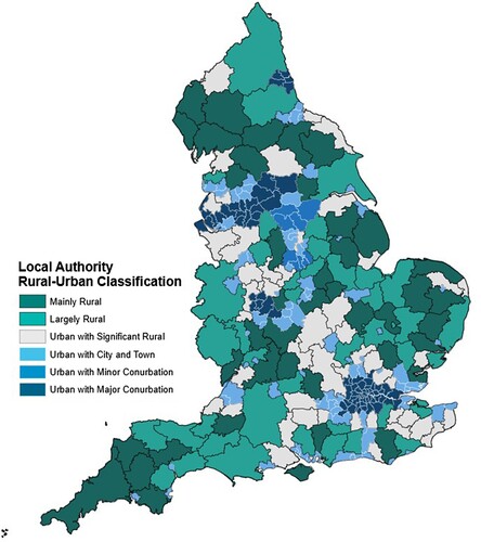
Under the 2011 Rural–Urban Classification for Local Authority Districts (LADs) in England, each LAD is assigned to one of six categories on the basis of the percentage of the total resident population accounted for by the combined rural and hub town populations, and its ‘conurbation context’ (a ‘hub town’ is a town of between 10,000 and 30,000 which serves a rural hinterland) (DEFRA, 2017a). The local authority categories are as follows:

• Mainly rural (population ≥ 80% rural including hub towns) (known as R80).

• Largely rural (population 50–79% rural including hub towns) (known as R50).

• Urban with significant rural (population 26–49% rural including hub towns).

• Urban with city and town (population < 26% rural including hub towns).

• Urban with minor conurbation (population < 26% rural including hub towns).

• Urban with major conurbation (population < 26% rural including hub towns).

The results of applying this classification to rural England are shown in Figure 1. It can be seen that mainly rural (R80) and largely rural (R50) districts tend to be further from urban conurbations. For example, Cumbria and Cornwall are mainly rural and Northumberland and Shropshire are largely rural. Urban with significant rural districts appear more diverse, including several around London but also districts in Somerset, Cheshire and Teesside.

Figure 1. English local authority districts (LADs) by rural–urban classification.

Source: DEFRA, RUC11, LAD21. © Crown Copyright and database rights 2023 Ordnance Survey Licence No. 100022861.

In a simplified version, DEFRA (2019, 2021) aggregates these six categories into three:

• Predominantly rural (≥ 50% of resident population lives in rural areas or hub towns).

• Significantly rural: officially ‘urban with significant rural’ since 2011 (26–49% of residents live in rural areas/hub towns). ‘Significantly rural’ is used here for clarity.

• Predominantly urban (≥ 74% of resident population lives in urban areas).

Some further insight into these categories may be helpful. According to DEFRA (2021), predominantly rural areas were home to 12 million people in 2020 (21.3% of the English population) and their population was growing and ageing faster than that of predominantly urban areas, largely due to internal migration. Specifically, the trend has been for net migration to predominantly rural areas and net migration from predominantly urban areas. This has been age-selective, such that between 2001 and 2015:

Predominantly Rural areas have proportionately seen large falls in the population aged 30 to 39 and higher proportional increases in the older population. The population aged 65 and over increased by 37% in Predominantly Rural areas, compared with 17% in Predominantly Urban areas

over this period (DEFRA, 2021, p. 25). Most of rural England is within commuting distance of urban employment opportunities, including most significantly rural areas, and some but not all of the predominantly rural areas.

To help decide whether to use the three- or six-category classification in the analysis, Table 1 presents the results of a logistic regression analysis in the form of mean marginal effects of place of residence. These estimates are interpreted as the change in the probability of being poor if the individual is living in a given area type compared with the reference category. The data in panel 1 show that for individuals living in rural areas (under the output area binary definition), the probability of being poor is 12 percentage points lower than for to those living in urban areas.

Table 1. Place of residence as a predictor of likelihood of poverty.

		Marginal effects
(1)	National Statistics Rural and Urban Classification of Output Areas released on 21 July 2004
	Rural resident dummy	−0.120***
(2)	Rural–Urban LA Classification (2011)
	Predominantly Rural	−0.062***
	Predominantly Urban (reference category)	–
	Significantly Rural	−0.104***
(3)	Rural–Urban LA Classification segregation London (2011)
	Predominantly Rural	−0.075***
	Predominantly Urban	−0.011
	Significantly Rural	−0.112***
	London (reference category)	–
(4)	Rural–Urban LA Classification (2011)
	Largely Rural (rural including hub towns 50–79%)	−0.081***
	Mainly Rural (rural including hub towns ≥ 80%)	−0.062**
	Urban with City and Town	−0.047***
	Urban with Major Conurbation (reference category)	–
	Urban with Minor Conurbation	−0.009
	Significantly Rural (rural including hub towns 26–49%)	−0.118***
(5)	Rural–Urban LA Classification segregating London (2011)
	Largely Rural (rural including hub towns 50–79%)	−0.075***
	Mainly Rural (rural including hub towns ≥ 80%)	−0.071**
	Urban with City and Town	−0.045***
	Urban with Major Conurbation	0.010
	Urban with Minor Conurbation	−0.003
	Significantly Rural (rural including hub towns 26–49%)	−0.112***
	London (reference category)	–
	Observations	11,646

Note: Presented are mean marginal effects from logistic regression models of the determinants of poverty. *p < 0.10, **p < 0.05, ***p < 0.01. LA, local authority.

Panel 2 focuses on the effects of residence using the three-category classification. Compared with persons living in predominantly urban areas, residents of predominantly rural local areas are 6.2% less likely to be poor and residents of significantly rural local areas are 10.4% less likely. In panel 3, London is distinguished from predominantly urban and made the reference category. These data show that the likelihood of being poor among urban residents is not statistically different from that of Londoners. Rural residents retain their significant advantage: in fact, it is slightly stronger.

Panel 4 examines the association between residence type and poverty using the full six-category residential taxonomy. While the various urban and rural categories differ in their association with poverty, the overall picture is quite similar to that produced using the three-category aggregation. The poverty rates of persons living in major and minor conurbations are not statistically different, although persons living in urban local areas that include a city or town are slightly less likely to be poor than their more highly urbanised counterparts. Living in a largely rural areas (R50) provides strong protection against poverty. Residence in mainly rural areas (R80) is also protective, but less so compared with largely rural R50 districts. Similar to the results shown in panels 2 and 3, residence in a significantly rural area provides the greatest protection against poverty, probably reflecting commuters’ access to better employment.

Panel 5 contains the same analysis but with London withdrawn from the urban with major conurbation category and used as the reference category. The results are very similar to those shown in panel 4. Perhaps the most interesting finding here is that poverty likelihood does not vary between Londoners and persons living in other major or minor conurbations. Similar to the data shown in panel 4, residents of urban local areas with a city or town are less likely to be poor than their more highly urbanised peers living in conurbations.

On the basis of this information, while the analysis has been conducted with both three- and six-category formulations, it is considered that presentation of the three-category analysis is sufficient for reporting the results in this paper, except in a few instances where further insights from the six-category analysis are especially worthy of mention.

2.3. Outcome variable

Poverty status is our outcome variable. This binary variable is equal to 1 if an individual has an equivalised household income (AHC) of less than 60% of England’s median household income. This is the widely accepted Eurostat operationalisation of the EU Council’s definition of poverty: ‘people are said to be living in poverty if their income and resources are so inadequate as to preclude them from having a standard of living considered acceptable in the society in which they live’ (Council of the European Union, 2004). To generate this variable, we follow usual practice in using annual net-equivalised household income AHC. Annual net household income is obtained from the household component of the USS assuming all members share the household resources. Hence, we assign each respondent the equivalised annual net household’s income using the McClements equivalence scales (Jones, 2007).

2.4. Explanatory variables: individual characteristics

Since we are studying individual poverty, we assign a number of household characteristics to the individual-level USS records. These variables have all been shown to be associated with poverty chances in previous research. We include categorical variables for the age of the head of the household, and dummy variables for different types of housing tenure (owned, mortgaged, rented, social housing), household type (single person, couple: no children, couple with children, lone parent, lives with other adults), economic activity of the household head (employment status and type of contract if employed), educational attainment of the household head, and for the number of employed people in the household.

Recent data on drivers of poverty in the UK are provided by Francis-Devine (2021) and the Joseph Rountree Foundation’s (JRF) (2022) recent report on poverty. These reports indicate that household poverty in the UK (including England) is higher in female-headed households, in households with younger heads, in households with young children, especially where only one parent is present, in households where the head has low educational attainment, in households that do not own their home, and in households with insecure labour market attachment.

More targeted research shows that age and gender are associated with the risk of poverty. Women, for example, are disproportionately poor in the UK (National Education Union, 2019) and children in sole parent families are especially vulnerable to poverty. In fact, relative child poverty increased from 27% in 2013–14 to 31% in 2019–20 (Cribb et al., 2022). Relatedly, younger households have higher poverty rates compared with mid- and later-career aged households (Trust for London, 2020a, 2020b). Educational attainment is strongly associated with lifetime earnings, and children whose parents have low educational attainment often attain relatively little education themselves. Hence low educational attainment contributes to intergenerational poverty (Centre for Longitudinal Studies, 2017; Thompson, 2020).

Poverty has been shown to be substantially lower among households that own their home compared with renters and residents of social housing (JRF, 2022; Trust for London, 2020). Research by the Institute for Public Policy Research (IPPR) (Murphy, 2018) showed that dramatic increases in property values have displaced many persons from home ownership to private renting or social housing. They estimate that one quarter of households will rent their housing by 2025. They also showed that housing costs among private renters have increased more than 50% faster than inflation over the past 25 years in the UK.

While poverty is lower among households with at least one employed person, research by IPPR shows that the protective effects of employment have declined in recent years. Poverty has increased substantially among employed persons, to the extent that in-work poverty now accounts for the majority of working-age households in poverty (McNeil et al., 2021) and the incidence of this is even higher in rural areas (Palmer, 2009). This reflected the impact of low wage growth, a lack of social housing and the rising cost of living, even before the energy crisis. Increased housing and childcare costs are major drivers of poverty among working families.

2.5. Austerity cuts and welfare reforms

These variables measure changes in governmental social welfare spending and austerity cuts at the LAD level. These LAD-level data are linked to individual respondent records. We include three key explanatory variables:

• Percentage decrease in core spending power between 2014/15 and 2018/19 as a measure of changes in revenue funding available to LADs to spend in any year. This variable is split into quartiles with the lowest quartile (q1) comprising households from a LAD with the smallest change in core spending power, and the highest quartile (q4) including households living in a LAD with the greatest decrease in core spending power.

• Percentage decrease in service spending between 2009/10 and 2016/17 at the LAD level. Service spending is a measure of actual revenue spending (not capital) by each local authority. To enable longitudinal comparison over the study period we exclude spending on education, police, fire, new public health grants and new responsibilities relating to social care. As with change in core spending power we allocate households into four different quartiles from smallest change (q1) to largest ones (q4), with the latter being the most affected by austerity cuts.

• Expected decline by 2020/21 in per capita income (£) because of cuts to welfare benefits at the LAD level. This variable combines real losses from pre-2015 reforms (as by March 2016) with estimated losses of all welfare reforms between 2010 and 1220 in March 2019.

These three categorical variables are divided into quartiles to assess non-linearity in spending cuts and welfare losses across the distribution (Table 2). Thus, for example, 8.4% of the predominantly rural population lived in LADs experiencing the greatest decrease in local government spending power between 2014/15 and 2018/19, compared with 26.3% of those living in predominantly urban areas, and 25.9% of the population residing in significantly rural areas. These data show that both urban and rural areas received diminished government spending between 2014/15 and 2018/19 with predominantly urban areas experiencing a greater loss.

Table 2. Changes in government spending and welfare in urban versus rural areas (%) and distribution across population quartiles.

(*100)	Predominantly Rural	Predominantly Urban	Significantly Rural
Real terms change in local government spending power between 2014/15 and 2018/19	−0.96%	−2.83%	−1.68%
Quartiles (*100-%)
Quartile 1	0.830	0.196	0.280
Quartile 2	No observations	0.246	0.371
Quartile 3	0.085	0.295	0.089
Quartile 4 (greatest decrease)	0.084	0.263	0.259
Real terms change in local government service spending between 2009–10 and 2016–17	−17.90%	−27.40%	−16.97%
Quartiles (*100-%)
Quartile 1	0.534	0.182	0.697
Quartile 2	0.228	0.242	0.303
Quartile 3	0.154	0.288	No observations
Quartile 4 (greatest decrease)	0.084	0.287	No observations
Total anticipated loss by 2020/21 from pre- and post-2015 welfare reforms (per capita)	£629.00	£800.00	£610.20
Quartiles (*100-%)
Quartile 1	0.62	0.18	0.84
Quartile 2	0.34	0.25	0.08
Quartile 3	0.04	0.27	0.07
Quartile 4 (greatest loss)	No observations	0.29	No observations
Observations	924	10,161	571

Note: Values for each quartile indicate the incidence of government spending and welfare cuts across local area districts by urban versus rural residence. Thus, for example, 29% of the predominantly urban population reside in local authority districts (LADs) with the greatest decrease in income because of welfare reforms between 2010 and 2020, compared with none in predominantly rural or significantly rural areas.

Source: Authors’ analysis of data from the Understanding Society Survey (USS) combined with government data (core spending power), Institute of Fiscal Studies (IFS) data (service spending), and information from the Centre for Regional Economic and Social Research at Sheffield Hallam University (welfare reforms).

3. POVERTY RATES, SOCIODEMOGRAPHIC CHARACTERISTICS, AND WELFARE CUTS IN RURAL AND URBAN ENGLAND

3.1. Poverty rates

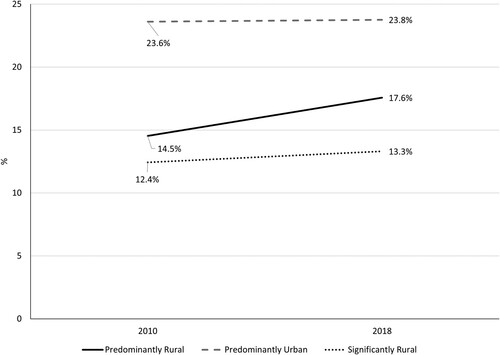
The share of urban and rural working-age individuals in poverty in 2010 and in 2018 from our analysis is shown in Figure 2. While our multivariate analysis is done in 2018 only, it is relevant to provide this descriptive information on 2010 to see how poverty rates changed over the past decade. In 2018, after the period of budgetary cuts and welfare reforms, poverty rates grew higher for both urban and rural populations, but while urban poverty continued to exceed rural in 2018, the gap between predominantly rural and predominantly urban rates areas narrowed from 9.1 in 2010 to 6.2 in 2018. This was due to the more rapid increase of poverty among predominantly rural residents during this period. Poverty rates increased by 21.3% in predominantly rural areas and by 7.2% in significantly rural areas. In contrast, the poverty rate was virtually unchanged in predominantly urban areas. Possible reasons for this narrowing of the rural–urban poverty gap between 2010 and 2018 are considered in the discussion section below.

Figure 2. Share of working-age individuals in poverty by rural–urban residence in England, 2010 and 2018.

Source: Authors’ analysis of data from the Understanding Society Survey (USS).

3.2. Comparative profile of sociodemographic characteristics

The USS data displayed in Table 3 show a comparative profile of individuals in England by rural–urban place of residence for 2018. These data show that persons living in predominantly urban areas are somewhat more likely to be characterised by attributes associated with a higher likelihood of being poor, discussed in Section 2.4 above. These individuals are more likely to have household heads with lower educational attainment, to reside in social or rented housing, and are more likely to have an unemployed head or a head that is economically inactive. In contrast, persons people living in significantly rural have characteristics that research shows to be negatively associated with the risk of poverty. For example, compared with the other two residential classifications residents of significantly rural areas are most likely to live in an owned or mortgaged house, have the highest employment and lowest unemployment rates, and have the highest percentage with a university degree. Persons living in predominantly rural areas are somewhat in between the other two categories.

Table 3. Sociodemographic and economic characteristics by place of residence, England, 2018.

	Predominantly Rural	Predominantly Urban	Significantly Rural
Head of household female	50.5%	43.9%	45.5%
Head of household age (years)
Head of household 16–24	2.2%	1.85%	1.06%
Head of household 25–55	69.2%	69.0%	70.4%
Head of household 56–65	22.8%	20.9%	24.0%
Housing tenure
Owned/mortgage	71.7%	65.1%	74.6%
Social housing	12.0%	20.1%	13.1%
Private rent	16.4%	14.8%	12.3%
Type of family
Single	10.5%	9.62%	11.3%
Couple, no children	21.5%	11.7%	19.6%
Couple, children	31.2%	28.7%	31.0%
Lone parents	4.39%	4.42%	5.11%
Other households	32.4%	45.6%	33.0%
Head of household economic activity
Employed	64.0%	60.1%	67.7%
Self-employed	13.8%	11.8%	11.5%
Unemployed	3.29%	5.33%	2.82%
Inactive	18.9%	22.7%	18.0%
Head of household education
University degree	30.6%	32.3%	33.5%
Other higher education	14.2%	12.0%	13.2%
A-levels	22.3%	17.8%	21.7%
GCSE	21.0%	17.8%	21.0%
Other qualifications	6.81%	8.86%	6.53%
No education	6.15%	8.85%	5.82%
Number of individuals employed in the household
0 persons	10.4%	9.62%	9.52%
1 person	26.5%	29.2%	26.8%
2 or more persons	63.1%	61.2%	63.7%
Observations	911%	9972%	567%

Source: Authors’ analysis of data from the Understanding Society Survey (USS).

While these descriptive data are suggestive of why urban poverty rates exceed their rural counterparts, they do not reveal whether living in an urban area, in and of itself, has an independent effect on the likelihood of poverty once these socio-demographic attributes are controlled in a multivariate analysis. In other words, will the ‘rural advantage effect’ persist after other covariates of poverty are controlled. Hence, the impacts of residence type and socio-economic factors on the likelihood of poverty merit multivariate analysis, and this is presented in Sections 4 and 5 below.

3.3. Austerity after the 2008 Global Financial Crisis

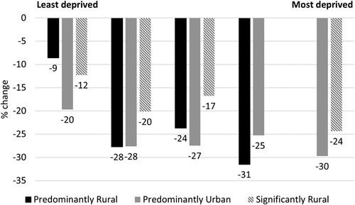
Public expenditure cuts from 2010 disproportionally affected the less well-off with welfare spending and local government particularly hard hit. Following May et al. (2020), we use IFS data on service spending cuts (Amin Smith et al., 2016) merged with our USS data to further distinguish how these cuts have affected rural versus urban areas. We allocate local authorities to five equal groups based on their average income deprivation domain scores of the 2015 index of multiple deprivation (IMD) (MHCLG, 2015). As shown in Figure 3, our results confirm May et al.’s (2020) findings that the most deprived areas experienced the greatest cuts in central government funding of local authorities in both urban and rural England. Note that there is no predominantly rural bar in the fifth quintile and no significant rural bar in fourth quintile because there were no cases of these LADs in those quintiles. This applies also to Figures 4 and 5.

Figure 3. Real terms change in local government service spending by 2005 index of multiple deprivation and rural–urban residence: England, 2009–10 to 2016–17 (% change).

Source: Authors’ analysis of data from the Understanding Society Survey (USS) and Institute of Fiscal Studies (IFS) data.

The pattern is largely the same with regard to local government spending power, as shown in Figure 4. Here we compare the core spending power of local authorities between 2014/15 and 2018/19 (MHCLG, 2019). Core spending power measures the core revenue funding available for local authority services, derived mainly from three sources: Council Tax (a local property tax); locally retained business rates (a tax on businesses related to turnover); and a revenue contribution from central government distributed according to a funding formula reflecting need. It should be noted that local authorities in England are not free to raise their own revenue as they wish (as they would be in most other countries): central government limits how much local taxes can increase each year as part of its limits on public expenditure. Over this period local authorities faced big reductions in their central government contribution which they have therefore been unable to offset by raising taxes locally.

Figure 4. England: real-terms change in local government spending power by 2005 index of multiple deprivation and rural–urban residence: 2014/15–2018/19.

Source: Authors’ analysis of data from the Understanding Society Survey (USS) and Ministry of Housing, Communities & Local Government (MHCLG) data.

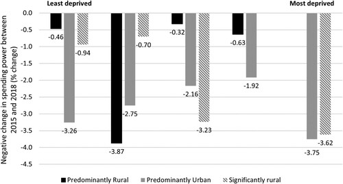
On average, core spending power was reduced by 2.8% in predominantly urban local authority areas and 2.1% in significantly rural areas, but only by 1.32% in predominantly rural areas. However, when disaggregated by level of deprivation, we observe that significantly rural areas have suffered similar reductions in their core spending power as their predominantly urban peers.

We next examine the total estimated loss resulting from all welfare reforms between 2010/11 and 2020/21 (data from Beatty, 2020; Beatty & Fothergill, 2018). In this analysis, we combine changes in benefit payments (financial loss per working-age adult, £/year) with our three category rural–urban classification and the IMD. Figure 5 shows the total estimated loss of per capita income due to welfare reforms between 2010 and 2015 and the anticipated loss from 2015 to 2020/21.

Figure 5. Decline in per capita income as a result of cuts to welfare benefits by 2005 by index of multiple deprivation and rural–urban residence.

Source: Authors’ analysis of data from the Understanding Society Survey (USS) and from Beatty and Fothergill (2018).

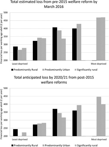
On average, urban residents are more likely than their rural peers to see a reduction in annual income as a result of welfare reforms (£800 anticipated loss by 2020/21 from pre- and post-2015 welfare reforms per working-age adult in predominantly urban areas compared with £629 for predominantly rural residents). However, consistent with the government service spending data shown in Figure 3, the data in Figure 5 show that the most deprived predominantly rural and significantly rural areas experienced similar financial losses to those of their urban counterparts. Hence, it is not so much the rural–urban divide but the deprivation status of the LAD that determines the extent of the financial losses. In summary, Figures 3–5 show that the severity of the different austerity measures and welfare reforms seem to have had similar adverse effects on poor households regardless of rural or urban residence.

4. MULTIVARIATE ANALYSIS OF THE EFFECTS OF RESIDENCE TYPE ON THE LIKELIHOOD OF POVERTY

Next, we explore the extent to which living in rural areas significantly decreases the likelihood of being poor (e.g., the ‘rural advantage effect’) net of other predictors of individual poverty introduced in the descriptive analysis. Thus, we start by estimating the likelihood of being poor with a non-linear (logit) model specified as: (1) $P_i=\alpha +{\beta }_1\mathrm{rura}{l}_i+{\beta }_2{X}_i+{\beta }_3\mathrm{austerit}{y}_i+{ϵ}_i$(1) where $P_i$ is the individual’s poverty status; $\mathrm{rura}{l}_i$ is the independent variable of interest that tests for the rural advantage effect; and $X_i\mathrm{and}\mathrm{austerit}{y}_i$ control for individuals’ socio-economic and demographic characteristics and characteristics of their spatial context, respectively.

We estimate stepwise models. Model 1 includes solely a dummy for the three category rural–urban residence variable with urban being the reference category (the raw ‘rural-advantage’). We provide additional evidence on whether this rural ‘advantage’ remains after controlling for individual’s demographic and socio-economic characteristics (model 2), and then consistent with our principal focus, model 3 examines the effects of changes in governmental social welfare spending and austerity cuts. Since poverty rates overall appear to be associated with changes in government social welfare spending and austerity cuts (Brewer et al., 2009; Vera-Toscano et al., 2020), we test how changes in government programmes since the introduction of austerity in 2010 are associated with the likelihood of being poor, and if the rural advantage persists after considering the effects of these policy changes.

4.1. Multivariate results

The data in Table 4 present results from the stepwise logistic regression examining the determinants of an individual in poverty. To ease interpretation, we report mean marginal effects. The data in column 1 show the base model of the ‘rural advantage’. In this baseline specification, there is a significant negative association between living in a rural area and the likelihood of being poor. For individuals living in predominantly rural areas, results indicate that the probability of being poor is 6.2 percentage points lower than for to those living in predominantly urban areas. For individuals living in significantly rural areas protection against poverty is even greater, for example, the probability of being poor is 10.4 percentage points lower than for people who live in predominantly urban areas. However, the question is whether this rural advantage is attributable to the characteristics of persons living in rural versus urban areas, or if the rural context per se diminishes the likelihood of poverty. Accordingly, models 2 and 3 control for individual and local authority characteristics thought to be associated with poverty.

Table 4. Predictors of poverty.

	Rural dummy	Rural dummy + Individual characteristics	Rural dummy + Individual characteristics + Local authority characteristics
Place of residence (ref. Predominantly Urban)
Predominantly Rural	−0.062***	−0.040***	−0.021
Significantly Rural	−0.104***	−0.079***	−0.059***
Individual characteristics
Head of household female		−0.025***	−0.026***
Head of household age (ref. Head of household 25–55)
Head of household 16–24		0.122***	0.123***
Head of household 56–65		−0.003	−0.004
Housing tenure (ref. Homeowner)
Social housing		0.143***	0.145***
Private rent		0.175***	0.175***
Type of family (ref. Couple, no children)
Single		0.093***	0.092***
Couple, children		0.169***	0.166***
Lone parents		0.218***	0.217***
Other households		0.080***	0.077***
Head of household economic activity (ref. Unemployed/inactive)
Head of household self-employed		0.005	0.004
Head of household permanent contract		−0.113***	−0.114***
Head of household fixed term contract		−0.107***	−0.108***
Head of household education (ref. No education attained)
Head of household university		−0.104***	−0.097***
Head of household other higher education		−0.056***	−0.051***
Head of household A-levels		−0.056***	−0.053***
Head of household GCSE		−0.035***	−0.034***
Head of household other qualifications		−0.039***	−0.038***
Number of individuals employed in household (ref. 1 person working)
0 person		0.024**	0.022**
2 people or more		−0.142***	−0.138***
Local authority characteristics^a
Negative change in spending power – quartile 2			0.004
Negative change in spending power – quartile 3			−0.013
Negative change in spending power – quartile 4 (greatest decrease)			0.006
Change in service spending – quartile 2			0.013
Change in service spending – quartile 3			−0.014
Change in service spending – quartile 4 (greatest decrease)			0.013
Total anticipated loss by 2020/21 from pre- and post-2015 welfare reforms (per capita) – quartile 2			0.031***
Total anticipated loss by 2020/21 from pre- and post-2015 welfare reforms (per capita – quartile 3			0.035***
Total anticipated loss by 2020/21 from pre- and post-2015 welfare reforms (per capita – quartile 4 (greatest loss)			0.050***
Observations	11,646	11,535	11,535

^a For the three austerity cuts and welfare reforms measures used the reference category is the quartile (q1) where service spending or government spending power decrease the least in relation to the previous reference year and where the losses due to welfare reforms were the smallest.

Presented are mean marginal effects from logistic regression models of the determinants of poverty.

*p < 0.10, **p < 0.05, ***p < 0.01.

Source: Authors’ analysis of data from the Understanding Society Survey (USS).

Model 2 adds measures of individuals’ socio-economic and demographic characteristics. The results shown in this analysis are consistent with previous research reviewed above. Individuals living in households whose head is aged 16 to 24 years old are three times more likely to be in poverty than those living in prime working-age households, those whose head is aged 25–55 years old. Educational attainment of the head of the household has a consistent negative association with the likelihood of poverty ranging from 9.7% to 3.8% lower compared with households whose head completed no education. Labour activity of the household head is also associated with the likelihood of poverty, for example, households whose head has a permanent or fixed term contract (compared with being out of the labour force) have a 10% lower likelihood of being in poverty. Households comprised of couples with no children have lower risks of poverty compared with other family types, especially lower than lone parents and couples with children. In contrast, not owning a house, increases the risk of poverty for household members. Home ownership decreases the risk of poverty by 14.5% compared with persons in social housing and 17.5% compared with renters. As expected, households lacking any employed members are significantly more likely to be in poverty than households with one employed member. Moreover, households with two or more employed members are 14% less likely to be poor compared with one worker households.

Importantly for this paper’s purposes, the rurality dummy remains significant after the inclusion of individuals’ socio-economic and demographic characteristics, although the ‘rural advantage’ for persons living in predominantly rural areas is reduced from 6.2% to 4.0%, and in significantly rural areas from 10.4% to 7.9%.

Model 3 (column 3) adds contextual (LAD) data on austerity cuts and welfare reforms that were linked with the USS survey respondents’ records. When these covariates are included in the model, the effect on poverty of living in a predominantly rural area while still negative is statistically insignificant. In other words, controlling for individuals’ socio-economic and demographic characteristics and local policy contexts eliminates any statistically significant difference in the likelihood of experiencing poverty between predominantly urban and predominantly rural residents. Controlling for individual and local authority characteristics also diminishes the rural advantage effect for individuals living in significantly rural areas, but such persons are still 5.9% less likely to be poor compared with their counterparts who live in predominantly urban areas. Hence, after accounting for demographic and local area characteristics, protection against poverty continues to be strong in local areas where 26–49% of population is rural. In contrast, such protection is substantially diminished in England’s most rural areas, for example, areas with lower access to urban economic opportunities.

Changes in local authority area spending power and service spending are not statistically associated with the likelihood of poverty among residents of such areas, after controlling for other variables. However, loss from welfare reforms does strongly significantly affect the likelihood of poverty. Controlling for rural–urban residence and individual and demographic characteristics, persons who live in areas with the highest per capita loss from welfare reforms are 5.0% more likely to be poor compared with persons living in areas with the smallest per capita welfare loss. In other words, the greater the loss due to welfare reforms (local authorities that are in the fourth quartile) the greater the likelihood of being in poverty. Moreover, the effects of individual and household characteristics remain virtually identical to those reported in model 2.

5. DISCUSSION, CONCLUSIONS AND UNANSWERED QUESTIONS

The primary aim of this paper has been to determine whether the ‘rural advantage effect’ in England persists once individual attributes associated with the risk of being poor, and cuts in welfare spending are accounted for in a multivariate analysis. To this end, a rural–urban classification of LADs in England was combined with USS data and LAD-level contextual data to enable the estimation of stepwise logistic regression models predicting the likelihood of being poor in 2018. Our results show that, after controlling for individuals’ socio-demographic characteristics and local policy contexts, the difference in the likelihood of experiencing poverty between predominantly urban and predominantly rural residents while still negative becomes statistically insignificant. In other words, once changes in austerity cuts and welfare reform are accounted for residents of predominantly rural LADs are no less likely to be poor that their counterparts living in predominantly urban areas. In contrast, residence in an urban area with significant rural population continues to give some protection against the risk of poverty.

Our results also shed light on which factors are responsible for the apparent rural advantage effect. Housing tenure is a key factor, with the much higher rates of home ownership in rural England affording protection against poverty, while tenants (especially private tenants) in rural and urban areas face greater expense and precarity. Labour market precarity is also a factor, with rural jobs increasingly casual, seasonal or otherwise insecure (Shucksmith et al., 2023), along with economic inactivity rates which may be indicative of diminishing local opportunity structures. While we lack direct information on commuting to urban jobs, it seems likely that residents of urban areas with significant rural populations (‘significant rural’) have more urban job access than their counterparts living in predominantly rural LADs.

One of the biggest factors, perhaps surprisingly, is the local impact of welfare reforms and austerity policies during the period which have had a very significant impact. Our analysis, consistent with other research, shows that austerity cuts were more severe in the poorest areas regardless of rural or urban residence. Interestingly, our further analysis suggests these cuts were more likely to lead to increases in poverty in rural England, while in urban England they were more likely to lead to increases in unemployment. Explanations for this difference in impacts will require further research.

This paper’s approach, combining spatial and micro-social data in logistic regression models, enables an understanding of which factors are responsible for the ‘rural–urban poverty gap’, specifically controlling for individuals’ socio-demographic characteristics and local policy contexts as well as types of rurality. Furthermore, the approach can be adapted to different national and regional contexts depending on availability of geo-referenced micro-data, a rural–urban classification scheme, and policy data that is reported at the local level.

These findings, and the underpinning analysis, will be of interest to those studying the ‘rural–urban poverty gap’ in many other countries around the world. While many nations consider socio-demographic characteristics in determining social programme eligibility, or how policies might affect the well-being of particular groups, few nations take rural–urban residence into consideration. For example, eligibility for the US’s Supplemental Food Assistance Program (SNAP) requires recipients to work or be enrolled in job training. While SNAP eligibility varies by age, family size, presence of children in the household and disability, where one lives is not considered (USDA-FNS, 2023). As a consequence of this one-size-fits-all approach, low-income persons living in rural areas who are more likely to have high unemployment, to lack job training facilities, or to provide public transportation to jobs or training facilities are systematically constrained from benefitting from SNAP. Our research shows the shortcomings of such spatially invariant programme designs. Clearly, social programme eligibility should be adjusted for spatial differences in opportunity structure, for example, for unemployment rates, if eligibility is contingent on work effort.

A secondary aim of this paper was to explore changes in working-age poverty rates in rural and urban areas through time, over the period since 2010, following the economic crisis and a change in government. Our results (see section 3.1) show that the gap between rural and urban poverty rates diminished between 2010 and 2018. While the urban poverty rate continued to exceed rural throughout, the gap between predominantly rural and predominantly urban poverty rates narrowed from 9.1 in 2010 to 6.2 percentage points in 2018, due to a more rapid increase of poverty among predominantly rural residents since 2010. Poverty rates increased by 21.3% in predominantly rural areas and by 7.2% in significantly rural areas, while the poverty rate was virtually unchanged in predominantly urban areas between 2010 and 2018.

While our analysis did not focus directly on the reasons for this faster growth of rural poverty since 2010, our analysis of factors associated with rural and urban poverty at the end of the period (2018), as well as research by other scholars, suggest several possible explanations which offer avenues for further research. For example, as shown by Palmer (2009), rural areas have much higher rates of in-work poverty compared with urban Britain, while other recent research (Asenova et al., 2015; JRF, 2022) indicates that working households have suffered some of the biggest cuts to welfare support. It may be that in 2010 rural areas contained more people earning just above the poverty line, for whom cuts in the real value of tax credits and other welfare support took them into poverty. It is also well established that eligible households in rural areas are less likely to claim their welfare entitlements (Bradshaw & Richardson, 2007) for various reasons including lack of access to advice and information, social stigma associated with welfare utilisation, and local cultures of independence and self-reliance (Shucksmith et al., 2023). May et al. (2020) point out that austerity policies led to the loss of many rural bus services, together with the consolidation and centralisation of job centres and citizens’ advice centres, all of which have made it harder to travel to work or to claim benefits.

Another likely explanation of the narrowing gap between rural and urban poverty rates is the pushing of poorer rural households into more expensive private rented housing due to a severe lack of social housing in rural England, along with the unaffordability of owner-occupation, at a time of rapidly rising market rents and cuts in welfare support for housing costs. Our analysis of data in the USS shows markedly different changes in housing tenure of low-income households in rural and urban Britain during 2010–18. The proportion of low-income households renting privately in rural Britain rose from 27.7% to 38.1% over this period, while the proportion in urban Britain was fairly stable, falling slightly from 38.7% to 37.8%. This striking difference came at a time when the cost of private renting grew rapidly to almost twice the cost of social housing or owner-occupation. This supports the hypothesis that the increased poverty rate (AHC) in rural England reflects a growing proportion of low-income households being forced into more expensive private rented tenure by a lack of more affordable alternatives.

In summary, poverty has increased throughout England since the 2008 recession, but the increase has been more rapid in rural areas. While rural residents continue to be less likely to be poor than their urban counterparts, the gap has diminished post-recession, and has been shown to reflect socio-demographic factors and the impacts of austerity policies and welfare reforms. Hence, people derive less protection from poverty by virtue of living in rural areas, and especially in predominantly rural areas, than was the case before 2010.

ACKNOWLEDGEMENTS

The authors are grateful to Andrew Williams and Christina Beatty for help with data sources, and to the editors and reviewers for their valuable comments. Thanks also to Bethany Kerwin of DEFRA for help with Figure 1.

DATA AVAILABILITY

The data analysed in this study are all publicly available: for the Understanding Society dataset, see https://www.understandingsociety.ac.uk/documentation; see https://www.gov.uk/government/publications/core-spending-power-final-local-government-finance-settlement-2019-to-2020 for local authorities’ core spending power, and see the Institute for Fiscal Studies (https://ifs.org.uk/publications/8781) for their service spending; for the data on the financial impact of welfare reforms, see https://www4.shu.ac.uk/research/cresr/ourexpertise/the-uneven-impact-of-welfare-reform; and for The Rural Urban Local Authority Classification data, see https://www.gov.uk/government/statistics/2011-rural-urban-classification-of-local-authority-and-other-higher-level-geographies-for-statistical-purposes/.

DISCLOSURE STATEMENT

No potential conflict of interest was reported by the authors.

Notes

1. We obtained access to a secure version of the USS dataset that contains the LAD code so that changes in government funding in the LADs where USS respondents reside can be linked to individual records. We were also able to append our rural–urban residence type classification to USS individual-level data by using the secure version of the USS managed by the University of Essex (University of Essex (ISER), 2020).

REFERENCES

- Amin Smith, N., Phillips, D., & Simpson, P. (2016). Real terms change in local government service spending by LA decile of grant dependence, 2009–10 to 2016–17. Institute of Fiscal Studies (IFS).
- Asenova, D., McKendrick, J., McGann, C., & Reynolds, R. (2015). Redistribution of social and societal risk: The impact on individuals, their networks and communities in Scotland. Joseph Rowntree Foundation (JRF).
- Beatty, C. (2020). Latest poverty map, updating Beatty C and Fothergill S (2017). https://twitter.com/CBeatty_CRESR/status/1488864256820928515
- Beatty, C., & Fothergill, S. (2018). Welfare reform in the United Kingdom 2010–16: Expectations, outcomes, and local impacts. Social Policy and Administration, 58(5), 950–968.
- Benzeval, M., Bollinger, C. R., Burton, J., Crossley, T. F., & Lynn, P. (2020). The representativeness of understanding society. Institute for Social and Economic Research.
- Bradshaw, J., & Richardson, D. (2007). Pension credit take-up in rural areas – State of the countryside update (SOC Update 4, December). Commission for Rural Communities (CRC).
- Brenner, N. (2004). New state spaces: Urban governance and the rescaling of statehood. Oxford University Press.
- Brenner, N. (2009). Open questions on state rescaling. Cambridge Journal of Regions, Economy and Society, 2(1), 123–139. https://doi.org/10.1093/cjres/rsp002
- Brewer, M., Muriel, A., Phillips, D., & Sibieta, L. (2009). Poverty and inequality in the UK. Institute for Fiscal Studies (IFS).
- Brown, D. L., Champion, T., Coombes, M., & Wymer, C. (2015). The migration–commuting nexus: Migration and commuting in rural England, 2002–2006: A longitudinal analysis. Journal of Rural Studies, 41, 118–128. https://doi.org/10.1016/j.jrurstud.2015.06.005
- Brown, D. L., & Schafft, K. A. (2019). Making a living in rural communities. In D. L. Brown & K. A. Schafft (Eds.), Rural people and communities in the 21st century: Resilience and transformation (pp. 205–229). Polity.
- Centre for Longitudinal Studies. (2017). Millennium cohort study briefing 13: Intergenerational inequality in early years assessments. https://cls.ucl.ac.uk/wp-content/uploads/2017/05/13_briefing_web.pdf
- Champion, T., Coombes, M., & Brown, D. L. (2009). Migration and longer-distance commuting in rural England. Regional Studies, 43(10), 1245–1259. https://doi.org/10.1080/00343400802070902
- Chapman, P., Phimister, E., Shucksmith, M., Upward, R., & Vera-Toscano, E. (1998). Poverty and exclusion in rural Britain: The dynamics of low income and employment. York Publ. Services.
- Commission for Rural Communities (CRC). (2010). State of the countryside 2010. CRC.
- Council of the European Union. (2004). Joint report by the Commission and the Council on Social Inclusion.
- Cribb, J., Waters, T., Wernham, T., & Xu, X. (2022). Living standards, poverty and inequality in the UK (Report No. R215). Institute for Fiscal Studies (IFS).
- Department for Environment, Food and Rural Affairs (DEFRA). (2017a). The 2011 rural–urban classification for local authority districts in England. Government Statistical Services.
- Department for Environment, Food and Rural Affairs (DEFRA). (2017b). The 2011 rural–urban classification for output areas in England. Government Statistical Services.
- Department for Environment, Food and Rural Affairs (DEFRA). (2019). Digest of rural statistics. HMSO.
- Department for Environment, Food and Rural Affairs (DEFRA). (2021). Digest of rural statistics. https://assets.publishing.service.gov.uk/government/uploads/system/uploads/attachment_data/file/1100175/07_Statistical_Digest_of_Rural_England_2022_August_edition.pdf
- European Society for Rural Sociology(ESRS). (2023). European Society for Rural Sociology XXIX Congress: Crises and the Future of Rural Areas, Working Group 11 on Spatial Inequalities. https://esrs2023.institut-agro-rennes-angers.fr/call-papers
- Flaherty, J., Veit-Wilson, J., & Dornan, P. (2004). Poverty – The facts. Child Poverty Action Group.
- Figari, F., Paulus, A., & Sutherland, H. (2015). The design of fiscal consolidation measures in the European Union: Distributional effects and implications for macroeconomic recovery. EUROMOD/Institute for Social and Economic Research.
- Francis-Devine, B. (2021). Poverty in the UK (Briefing Paper No. 7096, September). House of Commons Library. https://researchbriefings.files.parliament.uk/documents/SN07096/SN07096.pdf
- Fuguitt, G., Brown, D., & Beale, C. (Eds.). (1989). Rural and small town America. Russell Sage.
- Galster, G., & Sharkey, P. (2017). Spatial foundations of inequality: A conceptual model and empirical overview. The Russell Sage Foundation Journal of the Social Sciences, 3, 1–33. https://doi.org/10.7758/RSF.2017.3.2.01
- Gray, M. & Barford, A. (2018). The depths of the cuts: The uneven geography of local government austerity. Cambridge Journal of Regions, Economy and Society, 11(3), 541–563. https://doi.org/10.1093/cjres/rsy019.
- Hastings, A., Bailey, N., Bramley, G., & Gannon, M. (2017). Austerity urbanism in England: The regressive redistribution of local government services and the impact on the poor and marginalised. Environment and Planning A: Economy and Space, 49(9), 2007–2024. https://doi.org/10.1177/0308518X17714797
- Hills, J. (1995). Joseph Rowntree inquiry into income and wealth. Joseph Rowntree Foundation(JRF).
- Hobson, F. (2020). The aims of ten years of Welfare Reform (2010–2020) (Briefing Paper No. 9090, December). House of Commons Library. https://researchbriefings.files.parliament.uk/documents/CBP-9090/CBP-9090.pdf
- House of Commons Library. (2019). Poverty in the UK (Briefing Paper No. 7096, July). House of Commons Library. https://commonslibrary.parliament.uk/research-briefings/sn07096/
- Jones, F. (2007). The effects of taxes and benefits on household income, 2005/06. Office for National Statistics (ONS).
- Joseph Rowntree Foundation (JRF). (2021). Poverty report 2021. JRF.
- Joseph Rowntree Foundation (JRF). (2022). Poverty report 2022. JRF. https://www.jrf.org.uk/report/uk-poverty-2022
- Joyce, R., & Sibieta, L. (2013). An assessment of labour’s record on income inequality and poverty. Oxford Review of Economic Policy, 29(1), 178–202. https://doi.org/10.1093/oxrep/grt008
- Keen, R. (2016). Welfare Savings 2010/11 to 2020/21 (Briefing Paper No. 7667, July). House of Commons Library. https://researchbriefings.files.parliament.uk/documents/CBP-7667/CBP-7667.pdf
- Kitson, M., Martin, R., & Tyler, P. (2011). The geographies of austerity. Cambridge Journal of Regions, Economy and Society, 4(3), 289–302. https://doi.org/10.1093/cjres/rsr030
- Lobao, L. (2014). Economic change, structural forces and rural America: Shifting forces across communities. In C. Bailey, L. Jensen, & E. Ransom (Eds.), Rural America in a globalizing world (pp. 543–555). University of West Virginia Press.
- Lobao, L., Gray, M., Cox, K., & Kitson, M. (2018). The shrinking state: Understanding the assault on the public sector. Cambridge Journal of Regions, Economy and Society, 11(3), 389–408. https://doi.org/10.1093/cjres/rsy026
- Mather, M., & Jarosz, B. (2019). Demography and inequality. In D. Poston (Ed.), Handbook of population (second edition) (pp. 289–318). Springer.
- May, J., Williams, A., Cloke, P., & Cherry, L. (2020). Still bleeding: The variegated geographies of austerity and food banking in rural England and Wales. Journal of Rural Studies, 79, 409–424. https://doi.org/10.1016/j.jrurstud.2020.08.024
- McNeil, C., Parkes, H., Garthwaite, K., & Patrick, R. (2021). No longer managing: The rise of working poverty and fixing Britain’s broken social settlement. Institute for Public Policy Research (IPPR). https://www.ippr.org/files/2021-05/no-longer-managing-may21.pdf
- Ministry of Housing, Communities & Local Government (MHCLG). (2015). English indices of deprivation 2015. https://www.gov.uk/government/statistics/english-indices-of-deprivation-2015
- Ministry of Housing, Communities and Local Government (MHCLG). (2019). Local government revenue expenditure and financing statistics. https://www.gov.uk/government/collections/local-authority-revenue-expenditure-andfinancing
- Murphy, L. (2018). The invisible land: The hidden force driving the UK’s unequal economy and broken housing market. Institute for Public Policy Research (IPPR). https://www.ippr.org/research/topics/housing-infrastructure/?subtopic=affordable-housing&page_manualSearch=1
- National Education Union. (2019). Women and poverty. https://neu.org.uk/advice/women-and-poverty#:~:text=Women%20are%20more%20likely%20to,on%20in%20times%20of%20hardship
- Organisation for Economic Co-operation and Development (OECD). (2009). Poverty by individual and household characteristics. In OECD factbook 2009: Economic, environmental and social statistics (pp. 282–283). OECD Publ.
- Palmer, G. (2009). The poverty site. http://www.poverty.org.uk/summary/keyfacts.shtml
- Pateman, T. (2010). Rural and urban areas: Comparing lives using rural/urban classifications. Regional Trends, 43, 10–86. https://doi.org/10.1057/rt.2011.2
- Peck, J. (2013). Explaining (with) neoliberalism. Territory, Politics, Governance, 1(2), 132–157. https://doi.org/10.1080/21622671.2013.785365
- Peck, J., & Tickell, A. (2002). Neoliberalizing space. Antipode, 34(3), 380–404. https://doi.org/10.1111/1467-8330.00247
- Phillips, M. (1993). Rural gentrification and the processes of class colonisation. Journal of Rural Studies, 9(2), 123–140. https://doi.org/10.1016/0743-0167(93)90026-G
- Phimister, E., Shucksmith, M., & Vera-Toscano, E. (2000). The dynamics of low pay in rural households: Exploratory analysis using the British household panel survey. Journal of Agricultural Economics, 51(1), 61–76. https://doi.org/10.1111/j.1477-9552.2000.tb01209.x
- Pike, A., Béal, V., Cauchi-Duval, N., Franklin, R., Kinossian, N., Lang, T., Leibert, T., MacKinnon, D., Rousseau, M., Royer, J., Servillo, L., Tomaney, J., & Velthuis, S. (2023). ‘Left behind places’: A geographical etymology. Regional Studies, 1–13. https://doi.org/10.1080/00343404.2023.2167972
- Rabe, B. (2011). Geographical identifiers in understanding society (Understanding Society Working Paper Series). https://sp.ukdataservice.ac.uk/doc/6908/mrdoc/pdf/us_geographical_identifiers_nov11.pdf
- Rural Sociological Society (RSS). (1993). Persistent poverty in rural America. Westview.
- Shucksmith, M. (2000). Exclusive countryside? Social inclusion and regeneration in rural areas. Joseph Rowntree Foundation (JRF).
- Shucksmith, M. (2016). Social exclusion in rural places. In M. Shucksmith & D. Brown (Eds.), Routledge international handbook of rural studies (pp. 433–449). Routledge.
- Shucksmith, M., Glass, J., Chapman, P., & Atterton, J. (2023). Rural poverty today: Experiences of social exclusion in rural Britain. Policy Press.
- Thompson, I. (2020). Poverty and education in England. In I. Thompson, & G. Ivinson (Eds.), Poverty in education across the UK (pp. 115–140). Policy Press.
- Tickamyer, A., Sherman, J., & Warlick, J. (2017). Rural poverty in the United States. Columbia University Press.
- Trust for London. (2020a). Poverty before and after housing costs by age. https://www.trustforlondon.org.uk/data/poverty-by-age-group/
- Trust for London. (2020b). Poverty and type of housing. https://www.trustforlondon.org.uk/data/poverty-and-housing-tenure/
- University of Essex (ISER). (2020). Understanding society: Waves 1–10, 2009–2019 and harmonised BHPS: Waves 1–18, 1991–2009: Special licence access, local authority district. [data collection]. 12th Edition. UK Data Service. SN: 6666. https://doi.org/10.5255/UKDA-SN-6666-12
- USDA – Food & Nutrition Service. (2023). SNAP eligibility. https://www.fns.usda.gov/snap/recipient/eligibility
- Vera-Toscano, E., Shucksmith, M., & Brown, D. (2020). Poverty dynamics in rural Britain 1991–2008: Did labour’s social policy reforms make a difference? Journal of Rural Studies, 75, 216–228. https://doi.org/10.1016/j.jrurstud.2020.02.003
- Weber, B., Jensen, L., Miller, K., Mosley, J., & Fisher, M. (2005). A critical review of rural poverty literature: Is there truly a rural effect? International Regional Science Review, 28(4), 38. https://doi.org/10.1177/0160017605278996