An experimental study of methods for the analysis of variance components in the inference of laboratory information

Abstract

Measurement uncertainty (MU) can be estimated and calculated by different procedures, representing different aspects and intended use. It is appropriate to distinguish between uncertainty determined under repeatability and reproducibility conditions, and to distinguish causes of variation using analysis of variance components. The intra-laboratory MU is frequently determined by repeated measurements of control material(s) of one or several concentrations during a prolonged period of time. We demonstrate, based on experimental results, how such results can be used to identify the repeatability, ‘pure’ reproducibility and intra-laboratory variance as the sum of the two. Native patient material was used to establish repeatability using the Dahlberg formula for random differences between measurements and an expanded Dahlberg formula if a non-random difference, e.g. bias, was expected. Repeatability and reproducibility have different clinical relevance in intensive care compared to monitoring treatment of chronic diseases, comparison with reference intervals or screening.

Keywords:

• Dahlberg error
• repeatability
• reproducibility
• measurement uncertainty
• variance components
• analytical sensitivity

Introduction

Determination and monitoring of quality indicators are crucial and mandatory for measurements in laboratory medicine. The indicators which are primarily used are based on internal quality control (IQC) and external quality assessment/proficiency testing (EQA/PT), both relying on regular measurements of control materials. The frequency of control measurements is regulated by international or national standards and stated in the Standard Operating Procedures of accredited quality systems. Professional groups have discussed and outlined how quality goals [1,2] should be established in laboratory medicine to best serve clinical needs.

The typical IQC program consists of measuring control materials of known – or assigned – concentrations a certain times per day and assuming that the measurements of patient samples performed between control measurements are acceptable. Typically, control materials at two concentration levels are used. There is an abundance of commercial control materials available and critical properties of these are commutability with patient samples in the used measuring system, and stability over time. Alternatively, patient material can be used to investigate performance using duplicate measurements [3,4]. Using the latter approach, the entire measuring interval can be covered using native samples. A combination of different approaches and algorithms will provide comprehensive information about the performance of the method.

Quality indicators are designed to monitor the trueness and the precision of the measurement results and the quality systems designed to ensure that results are consistent, comparable over time and transferable between service providers. Laboratories need to have detailed information on trueness and precision whereas the clinician, assuming a sufficient analytical quality, appropriately will focus on the transferability and comparability of results to reliably identify differences between results and between patient values and reference values. In the present study, we compare various procedures using control materials and patient samples to estimate measurement uncertainty, compare the usefulness of the results and use simulations to estimate the number of necessary duplicate samples for repeatability estimates.

Methods and materials

Measuring system

All measurements were using Roche Diagnostics (Germany) Cobas c501 employing reagents from Roche ALTLP (Alanine Aminotransferase PyP) Ref 04467388190, ALP2S (ALP IFCC Gen.2) Ref 03333752190 and CA2 (Calcium Gen. 2) Ref 05061482190.

Stabilized control materials

The low and high concentrations reference materials were Autonorm Human Liquid L-1 1606342 and Autonorm Human Liquid L-2 1608804 (Sero A/S Oslo, Norway), respectively. These materials are based on human serum with no preservatives or stabilizers added, for maximum commutability.

Patient materials

De-identified patient samples from the laboratory routine production were used. The selected analytes were P-ALT (Plasma-Alanine transferase), P-ALP (P-Alkaline phosphatase) and P-Calcium. The Swedish law of biobanking (SFS 2002:297) allows the use of anonymized samples for quality development and management. The results of the present study can never be traced to any individual or group of individuals. Accordingly, the study did not require scrutiny by the Ethics committee.

Experimental design

All calculations and estimations were based on the following experimental designs (Figure 1).

Figure 1. The components and design of the study.

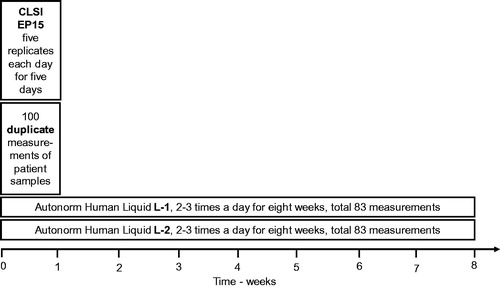
1. Control material of two concentrations were measured five times daily for five days and the ‘analysis of variance components’ (ANOC) was carried out in a 5 × 5 experimental design according to Clinical and Laboratory Standards Institute (CLSI) EP15 [4,5] in a specially developed MS Excel program [6]. This allows identifying the repeatability (within series variation), the ‘pure’ between series variation and the total variation (Figure 2).

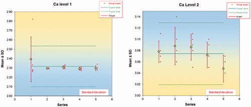
Figure 2. Within and between series variations based on series of five measurements on five occasions (days). One of the results (as shown in the figure) in the first series was regarded as an outlier and not used for further calculations.

2. Control materials of two concentrations were measured repeatedly, up to three times per day, totally 83 measurements of each quantity. The average, standard deviation (s) and %CV were calculated using standard procedures (Table 2).

3. The standard deviation was calculated from duplicate measurements of 100 consecutive patient samples, using the Dahlberg formula. The results of the expanded Dahlberg formula (ExpD) [4] were also calculated (Table 3).

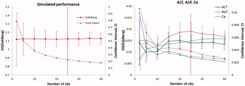
4. The standard deviation (Dahlberg, s_D) and the confidence intervals were calculated using the available ‘100-series’ of P-ALT, P-ALP and P-Calcium (P-Ca) (Figure 3), right panel. In creating these graphs, differences outside the average difference ±3 standard deviations of the differences were disregarded as not representative of the sample population.

Figure 3. Left panel. The standard deviation (target value 1.12) and confidence interval calculated by the simulation model 5. Each number of observations was simulated 100 times. The vertical line represents the suggested minimal number of observations needed. The corresponding graphs from the other simulations followed the same pattern. Right panel. Standard deviations for ALT, ALP and Ca were calculated using the 100 duplicates using the Dahlberg formula. Solid lines are standard deviations, dotted lines confidence intervals.

All calculations and data handling were performed using EXCEL 2016.

Calculations

The analysis of variance components (ANOC) requires an experimental design in which observational results can be identified as within-groups and between-groups. This is also the design of an one-way ANOVA which yields the sum of squares and mean squares (MS) of the observations within- and between groups [7,8]. We used a model with five measurements within the groups, i.e. obtained under repeatability conditions and carried out on five occasions, i.e. under reproducibility conditions. This is summarized as a 5 × 5 table. The within-group mean square (MS_w) is equal to the variance of the measurements within a group. The between group mean square (MS_b) is a combination of the ‘pure’ between group variance and the within group variance. The pure between group variance $s_b^2$ was obtained by (1) $$s_b^2=\frac{{MS}_b-{MS}_w}{n_0}$$(1) where n₀, is the average number of observations the groups. This is considered applicable in normal laboratory work and a reasonably balanced study.

The total or intra-laboratory variance $\left(s_{\mathit{tot}}^2\right)$ is (2) $$s_{\mathit{tot}}^2=s_b^2+{MS}_w$$(2)

If $\frac{{MS}_b-{MS}_w}{n_0}$ < 0, i.e. $\left({MS}_b<{MS}_w\right)$ then $s_{\mathit{tot}}^2={MS}_w,$ i.e. the within series variance [4].

The ANOC was also applied to the IQC data, assuming repeatability within days and reproducibility between days.

Imprecision was calculated from repeated measurements of control materials by the general formula for standard deviation (Equation (3)(3) $${\mathrm{ }s}^2=\frac{\sum _{i=1}^n{\left(x_i-\overline{x}\right)}_i^2\mathrm{ }}{n-1}$$(3) ); the Dahlberg formula [3,4] (Equation (4)(4) $$s^2=\frac{\sum _{i=1}^N{d}_i^2}{2\times \mathrm{N}}$$(4) ) was used for calculation of the repeatability assuming only a random variation between the original and replicate measurement and an expanded Dahlberg (ExpD) formula (Equation (5)(5) $$s^2=\frac{\sum _{i=1}^N{\left(d_i-\overline{d}\right)}^2}{2\times \left(N-1\right)}$$(5) ) [4] when a non-random variation between the results was assumed. (3) $${\mathrm{ }s}^2=\frac{\sum _{i=1}^n{\left(x_i-\overline{x}\right)}_i^2\mathrm{ }}{n-1}$$(3) (4) $$s^2=\frac{\sum _{i=1}^N{d}_i^2}{2\times \mathrm{N}}$$(4) (5) $$s^2=\frac{\sum _{i=1}^N{\left(d_i-\overline{d}\right)}^2}{2\times \left(N-1\right)}$$(5) where s² is the variance, n is the number of observations, N is the number of pairs in a comparison of duplicates and d is the difference between duplicates.

Simulations

Five different situations were identified in which duplicate measurements may be used for estimating the repeatability of a measurement procedure. In all examples, the bias was assumed to be negligible and the expanded Dahlberg results therefore not calculated. These simulations were undertaken to determine the minimal number of observations to achieve a reliable estimate of the Dahlberg standard deviation.

1. The original and replicate measurements were simulated by adding a random difference to a simulated normally distributed series of results with an average of 25 units and a standard deviation of 2 units, using the algorithm ‘average+s×NORM.S.INV(RAND())’ [9]. The average and standard deviation of an increasing number of draws were calculated. The corresponding real case occurs if a series of the same sample were measured in duplicates and their differences normally distributed.

2. Random values between 23 and 27 units (25 ± 2 units) were chosen as original observations, i.e. a rectangular distribution with a measurement interval of 4 units and a random difference between −5 and +5 added, i.e. a standard deviation of $5/\sqrt{3}=2.89 \mathit{units}.$ The corresponding real case would be a measurement procedure where the results differ randomly within a defined interval.

3. The original measurements were simulated as a normal distribution. The replicates were made dependent and the difference between the original and replicate was normally distributed with a constant standard deviation, i.e. ‘s×NORM.S.INV(RAND())’ and no bias assumed. This mimics a homoscedastic profile.

4. The original observations were randomly chosen within the interval 10 to 30 units. The differences were randomly chosen between (−3) and (+3), i.e. the standard deviation estimated to $3/\sqrt{3}=1.73 \mathit{units},$ assuming a rectangular distribution. The repeatability was calculated from the differences between the replicates and the originals, expressed in relation to the average of the original and replicate.

5. The original series was a set of randomly chosen numbers between 10 and 30 units. The replicates were created as a function of the original and a randomly chosen proportionality factor between 1.005 and 1.025 and therefore dependent on the original observation. The relative differences between the original and the replicate were used to calculate the standard deviation. This mimics a heteroscedastic profile.

The target value was defined as that obtained by simulation of a sufficiently large number of observations. In the present study, a target value of 1.12 was obtained as the average of 100 simulations of 40 observations.

Based on these assumed situations, five sets of simulations were made, each comprising 50 samples. The Dahlberg formula was applied to two, three, four and so of pairs of the dataset. Results of standard deviations based on 2, 5, 10, 15, 20, 25, 30, 35 and 40 pairs were then tabulated and repeated 100 times. The average of the variances which were calculated this way and their confidence intervals are shown in Figure 3, left panel.

To investigate the influence of bias on the calculations and to illustrate the difference between the Dahlberg formula and the ‘expanded Dahlberg’ formula, appropriate series of 0.5 × 10⁶ observations were simulated. The average of the ‘original’ series was set to 10 with a standard deviation of 1, thus defining the measuring interval. The random error to create the ‘repeat’ value was based on a normal distribution with an average of zero and a coefficient of variation of 2.5% or 5.0%. As a third series, the ‘repeat’ series was modified by adding a constant error ranging from 1 to 20% of the average of the original series of measurements. This represents a bias or systematic variation between the original and repeat measurements.

Results

Analysis of variance components using reference materials

Results of the ANOC are exemplified in Figure 2 using the results from the two calcium reference materials measured 5 × 5 times. There was one outlier in the first series of the low concentration. This observation was not included in the calculations but the results are included for the sake of information. The results of ALT, ALP and Ca are summarized in Table 1. In all experiments the within series (repeatability) was the dominating source of uncertainty. In the series of low Ca-concentration the mean square of the reproducibility (between series) was lower than that for the repeatability and therefore set to zero [10]. The total variance is the sum of the repeatability and the ‘pure’ between series variances. The relative intra-laboratory standard deviation was about 1% for the three studied quantities (Table 1).

Table 1. Details of analysis of variance components.

	ALT Level 1	ALT, level 2	ALP Level 1	ALP Level 2	Ca Level 1	Ca Level 2
Between series df	4	4	4	4	4	4
Within series df	20	20	20	20	19	20
Number of observations	25	25	25	25	24	25
Average	0.73	2.32	1.38	4.93	2.29	3.07
SEM	0.002	0.004	0.003	0.011	0.004	0.005
Repeatability (s)	0.009	0.021	0.016	0.054	0.021	0.025
Pure between series (s)	0.005	0.001	0.005	0.010	–	0.012
Total imprecision (s)	0.011	0.021	0.017	0.055	0.021	0.028
Repeatability (%CV)	1.3	0.92	1.2	1.1	0.90	0.81
Pure between series (%CV)	0.63	0.05	0.36	0.20	–	0.38
Total imprecision (%CV)	1.45	0.93	1.22	1.11	0.90	0.89

The outlier shown in Figure 2 was excluded from the summary calculations. The ‘pure between series imprecision’ was obtained by correcting the between group ‘mean square’ of the ANOVA analysis [4] for the contribution of the repeatability variance. The between group mean square (MS_b) was smaller than that of the within group for the Ca-measurements of the low concentration material and therefore not presented.

Reproducibility by IQC

The average and standard deviation were calculated by standard methods, across all results, of the daily measurements of control materials and shown in Table 2. Since the results were collected during an extended period of time, they were regarded as obtained under reproducibility conditions and in this case also representing intra-laboratory uncertainty or total imprecision.

Repeatability, pure reproducibility and total uncertainty were also calculated from the IQC observations. For the high concentration materials of all analytes and the low concentration material for calcium the MS_b proved smaller then MS_w and the total variance therefore equal to the repeatability. The variance across all observations was equal to that calculated by analysis of variance components.

Table 2. The imprecision (standard deviation) calculated across all observations and using the method of analysis of variance components from 2 to 6 daily IQC measurements of control material, comprising 83 observations.

	ALT µkat/L		ALP µkat/L		Calcium mmol/L
Average	0.74	2.32	1.38	4.95	2.29	3.08
Across (s)	0.013	0.021	0.020	0.054	0.018	0.021
%CV	1.76	0.90	1.42	1.09	0.77	0.66
Repeatability (s)	0.009	0.022	0.017	0.054	0.018	0.021
Pure Reproducibility (s)	0.009	–	0.009	–	–	–
Intra-laboratory (s)	0.013	0.022	0.020	0.054	0.018	0.021

Repeatability imprecision estimated by duplicate measurements

The P-ALT, P-ALP and P-Ca concentrations were measured as duplicates in 100 consecutive routine samples. Only the first value was reported to the clinic to be used in patient care. The duplicate results were analyzed by the Dahlberg formula and the ExpD [4,11], (Table 3). Since the s(X)(Dahlb) and s(X)(ExpD) are virtually identical no bias could be demonstrated between the original and repeat measurements.

Table 3. Properties of duplicate measurements of patient samples.

	ALAT	ALP	Ca
Count	100	100	100
Average	1.84	3.46	2.32
Median	0.69	2.05	2.36
IQR	25.00	75.00	75.00
10 percentile	0.37	1.41	2.21
90 percentile	1.71	4.70	2.47
Maximum observations	10.3	16.6	3.2
Minimum observations	0.1	0.5	1.3
s(X) (Dahlb)	0.016	0.023	0.016
%CVD(X)	3.26	0.69	0.72
Maximum difference	0.10	0.11	0.06
Average difference	0.0004	−0.0002	−0.0008
Student tdep	0.17	0.06	0.35
p (2-tail)	.863	.951	.729
s(X) (ExpD)	0.016	0.023	0.016

The repeatability (bold) was calculated by Dahlberg’s formula and the expanded formula (ExpD). s(X) and %CV(X) represent the absolute and relative Dahlberg uncertainty, respectively.

Necessary sample size

The five simulated models differed with respect to the design of the measuring interval and the relation between the original and repeated results. The original results were either normally distributed with limited tails or taken from a rectangular distribution. The repeated results were either obtained by the addition of a random number for a normal distribution or obtained by multiplication with a random, reasonable factor. Therefore, the original and repeat results were related in a defined fashion. As expected, the estimated standard deviation approached the target value as the number of included pairs increased and its variance and confidence interval decreased. Beyond 25 pairs, the standard deviation stabilized and a further decrease of the confidence interval was small. Similar results were obtained for all the simulation models (Figure 3).

Simulations with non-random variations

The large number of simulated data underpinning the Table 4 provides robust numbers for illustration of the influence of a non-random difference between the first and repeat observations. The first measurements were a series of 0.5 × 10⁶ values drawn from a normal distribution. The series of repeat results was obtained by adding a random number to the original. The averages of the first and repeat measurements were thus identical and the average difference was zero (Table 4). In a third series, a constant was added to the repeat series and therefore the difference between these series and the original is the bias. If the standard deviation was calculated using formula (Equation (3)(3) $${\mathrm{ }s}^2=\frac{\sum _{i=1}^n{\left(x_i-\overline{x}\right)}_i^2\mathrm{ }}{n-1}$$(3) ) after addition of the bias, it amounted to 2.0304 whereas if formula (Equation (5)(5) $$s^2=\frac{\sum _{i=1}^N{\left(d_i-\overline{d}\right)}^2}{2\times \left(N-1\right)}$$(5) ), ‘extended Dahlberg’ was used the same estimate was obtained as for the un-biased series. The simulated series were also subjected to evaluation by ANOC. The repeatability was the same as that obtained by the Dahlberg formula.

Table 4. Summary of the simulations of a normally distributed set of 0.5 × 10⁶ simulated results (Orig) from an average of 10 and a standard deviation of 1 and a simulated repeated series with an assumed average difference of 0.25 times a random normality probability function (Rep).

	Basic	Rand add		Non-rand	Bias add	Basic	Rand add		Non-rand	Bias add
	10	1	0.25	0		10	1	0.25	2
Set values	Orig	Rep	Diff	Rep + bias	Diff	Orig	Rep	Diff	Rep + bias	Diff
$\overline{x}$	9.9993	9.9992	−0.0001	9.9992	−0.0001	9.9987	9.9983	−0.0004	11.9983	1.9996
Sumsq(x1–x2)	5491200	50521745	31249	50521745	31249	50485271	50512924	31265	72508976	2030396
Stand dev (s)	0.9993	1.0306	0.2500	1.0306	0.2500	0.9996	1.0309	0.2501	1.0309	0.02501
Var Dahlberg			0.0313		0.0313			0.0313		2.0304
Var Expanded					0.0313					0.0313

A non-random difference, equal to zero and 2 (20%), right panel illustrates how a traditionally calculated SD_Dahl differs from that using the expanded Dahlberg formula, which gives an SD_ExpD devoid of an influence of the average of the bias. Finally, calculated quantities are in bold. The negligible effect of a random error between the original and repeated measurement is clearly shown as the variance of the repeats as the sum of the variances of the difference and original series (see text).

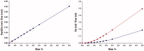
The absolute difference between a standard deviation estimated by the Dahlberg formula and the extended version of the Dahlberg formula is linear in relation to the relative size of the bias and independent on the measuring interval. The relative difference between the standard deviation estimated by the two formulas is related to the size of the non-random variation (Figure 4, right)

Figure 4. The difference between the Dahlberg standard deviation and that of the Dahlberg expanded formula (as the square root of the difference between the variances), left panel. The difference is linearly related to the relative bias and independent of the assumed random variation of the samples. The ratio (right panel) between the standard deviation estimated by the Dahlberg and Expanded Dahlberg formulas. The random difference between series was 2.5%.

Discussion

Different strategies to determine the measurement uncertainty in a medical laboratory were investigated. The uncertainty is linked to the measurement method as a method uncertainty and this concept is commonly recognized as a characteristic that should meet relevant quality goals. The standard uncertainty is by definition expressed as a standard deviation and therefore related to the dispersion of repeated measurements. However, in laboratory medicine samples may be from the same patient and the object of the measurement is to verify a difference between the samples. Since the samples may have been collected under different circumstances, the laboratory needs to consider establishing different measurement uncertainties for use in appropriate situations. Monitoring an acute clinical situation e.g. a potential myocardial infarction with Troponin is performed under repeatability conditions whereas for instance screening for a disease by comparing a result with a reference value or monitoring a chronic disease are considerred as performed under reproducibility conditions. The analytical sensitivity i.e. ability to verify a difference between results, increases as the uncertainty decreases. Consequently, there is not a single analytical quality goal and no single optimal method for expressing and monitoring analytical performance appropriate in all clinical contexts. In most cases, the repeatability uncertainty is less than the reproducibility uncertainty which is influenced by numerous factors. That does not exclude the possibility that the ‘pure’ reproducibility may be smaller than the repeatability. It is important for the laboratory to identify all sources of uncertainty to control causes of variability, minimize uncertainty and initiate corrective actions and differentiation of the uncertainty, e.g. recognizing the repeatability and reproducibility are valuable pieces of information.

Repeatability conditions are unchanged conditions i.e. using the same procedure, reagents, calibration, temperature etc. This is also known as the within series conditions. The within series uncertainty or simply ‘repeatability’ can be determined by repeated measurements of a control material under suitable constant conditions. If these ‘within series’ measurements are repeated, e.g. in a common IQC procedure, the repeatability and the reproducibility can be calculated using an ANOVA, analysis of variance components. The relevance of this information applies to the concentration of the used material only and is not necessarily representative for the entire measuring interval. Furthermore, the variance of variance components estimates depend on the underlying distributions [12,13]. The Dahlberg formula is derived differently and allows calculating the repeatability from duplicates of many samples of different concentrations [14]. A key question is how many replicates would be necessary to achieve a robust estimate of the uncertainty. Through simulation, we estimated the minimal number to 25 repeated samples. This was verified in original measurements of patient samples.

The Dahlberg formula (Equation (4)(4) $$s^2=\frac{\sum _{i=1}^N{d}_i^2}{2\times \mathrm{N}}$$(4) ) assumes a negligible variation of the uncertainty of the tested results or that the differences between the first and repeat observadtion are random, i.e. normally distributed. If this is not the case there is a systematic difference between the first and repeat measurement, i.e. a bias. This can be handled by the expanded Dahlberg formula which is the sum of squares of the differences between observed differences and the average of all differences. If there is no bias, the results of the formulas will coincide and it is therefore a good practice to apply both, which allows the bias to be quantified.

If repeatability conditions are not fulfilled, reproducibility conditions exist i.e. one or more measurement conditions have been changed. By necessity, the reproducibility ‘includes’ repeatability and to calculate the correct intra-laboratory variance, the ‘pure’ reproducibility should be calculated. The total or intra-laboratory variance can then be calculated as the sum of the two variances. This value can be compared to the variance calculated across all values. Particularly if the pure reproducibility is of a noteworthy size, the variance calculated across the values underestimates the intra-laboratory variance.

The principle of ANOC is a powerful tool for investigating the performance of a measurement method. It requires a special experimental setup to ensure that both repeatability and reproducibility conditions are studies. The technique has been adopted by the CLSI EP15 to verify the quality claims of a manufacturer [5]. Their setup is limited to 5 × 5 observations with the warning that the power of the used degrees of freedom is not sufficient to establish, only verify a method variance. A similar approach is used in the CLSI EP5 [15]. The technique has also been used in real time monitoring the comparability and performance of several laboratories which allows identifying problems within the individual laboratories and between those participating [16].

The repeatability imprecision was estimated by the Dahlberg formula (Table 3). There are numerous situations where, and reasons why, non-random differences between repeated measurements occur, e.g. carry over, reagent decay i.e. the experimental conditions are not truly repeatable. It is essential to design an experimental model which minimizes any systematic difference due to laboratory factors, i.e. bias, between the first and repeat measurements. In the present method and modelling study we have not considered any influence of pre-analytical variation. In large enough series the averages of the original and repeat observations coincide. This indicates a technique to estimate any bias either by simply comparing the averages of the series or applying the Student’s paired t-test. It is possible to estimate the bias also by applying and comparing the extended Dahlberg formula to the data. In the present study the two variances were equal and thus no bias between the two results. This was verified by the Student’s test for paired observations which supports the null hypothesis that there was no difference between the first and second results (Table 3). An overestimation of the repeatability imprecision by the Dahlberg formula was reported by Springate [17] which could possibly have been be caused by a non-random difference.

The expanded Dahlberg formula compensates for the non-random error and estimates the within series variation correctly (Table 4) in the presence of a bias between duplicates. It was shown in the simulation that the original Dahlberg formula will overestimate the repeatability in the presence of a bias, i.e. include the bias in the uncertainty estimate. The ANOC is liable to the same effects. The relative difference between the two estimates increases almost exponentially up to a relative bias of about 1.5% and subsequently increases almost linearly (Figure 4, right panel), whereas the square root of the difference between the calculated squared Dahlberg and Expanded formulas increases linearly. The magnitude of the ratio between the two estimates is also related to the measuring interval.

Conclusions

Analytical goals are conventionally defined according to a hierarchy agreed by the laboratory professions. The degree to which laboratories and accreditation bodies meet the requirements is often judged by evaluating measurements of control materials without considering their commutability with patient samples. Duplicate measurements of patient material for establishing and monitoring performance can be an option.

The analytical quality goals commonly do not differentiate between the repeatability and reproducibility and it is less obvious how the laboratories should measure the real uncertainty of measurements. As investigated in the present study, the uncertainty can be determined under repeatability and reproducibility conditions and it is argued that both are important for the laboratory and for the end-users of the results.

The experimental design to determine the quantities is critical and the clinical use of the information depends on the clinical situation. Evaluation of biochemical markers for a fast-changing disease should preferably rely on the repeatability whereas a slow process or trend should rather be based on the reproducibility or combined intra-laboratory variation. The laboratory can use the detailed information of variance components for quality control and rational corrective actions. In general, the repeatability uncertainty is smaller than the reproducibility or intra-laboratory uncertainty and therefore offers a more sensitive diagnostic tool.

Correction Statement

This article has been republished with minor changes. These changes do not impact the academic content of the article.

Disclosure statement

No potential conflict of interest was reported by the authors.

Additional information

Funding

This study was supported by the Karolinska university laboratory and the County council of Östergötland.

References

- Kallner A, McQueen M, Heuck C. The Stockholm Consensus Conference on quality specifications in laboratory medicine, 25-26 April 1999. Scand J Clin Lab Invest. 1999;59:475.
- Panteghini M, Sandberg S. Defining analytical performance specifications 15 years after the Stockholm conference. Clin Chem Lab Med. 2015;53:829–32.
- Dahlberg G. Statistical methods for medical and biological students. London: G. Allen & Unwin; 1940.
- Kallner A, Theodorsson E. Repeatability imprecision from analysis of duplicates of patient samples. Scand J Clin Lab Invest 2020;80(1):73-80.
- CLSI. EP15-A3. User Verification of Performance for Precision and Trueness Approved Guideline - Third Edition. Wayne, PA: Clinical and Laboratory Standards Institute; 2014. Standard No.: ISBN 1-56238-000-0.
- Kallner A. Measurement verification. [cited 2019 May 8]. Available from: http://www.acb.org.uk/whatwedo/science/best_practice/measurement_verification/measurement-verification-2018
- Aronsson T, Groth T. Nested control procedures for internal analytical quality control. Theoretical design and practical evaluation. Scand J Clin Lab Invest Suppl. 1984;172:51–64.
- ISO. Accuracy (trueness and precision) of measurement methods and results - part 2: basic method for the determination of repeatability and reproducibility of a standard measurement method. Geneva: International Standards Organisation; 1994. Standard No.: ISO/DIS 5725-2:1994.
- Kallner A. A study of simulated normal probability functions using Microsoft Excel. Accred Qual Assur. 2016;21:271–76.
- Kallner A. Laboratory statistics: handbook of formulas and terms. 2nd ed. ISBN: 978-0-12-814348-3. Amsterdam: Elsevier; 2018.
- Hyslop NP, White WH. Estimating precision using duplicate measurements. J Air Waste Manag Assoc. 2009;59:1032–39.
- Tukey JW. Variances of variance components: II. The unbalanced single classification. Ann Math Statist. 1957;28:43–56.
- Tukey JW. Variances of variance components: I. Balanced Designs. Ann Math Statist. 1956;27:722–36.
- Kallner A, Petersmann A, Nauck M, et al. Measurement repeatability profiles of eight frequently requested measurands in clinical chemistry determined by duplicate measurements of patient samples. Forthcoming. 2019.
- CLSI. EP5-A3. Establishment of Precision of Quantitative Measurement Procedures; Approved Guideline—Third Edition. Wayne, PA: CLSI; 2014. Standard No.: ISBN 1-56238-000-0.
- Ayling P, Hill R, Jassam N, et al. A practical tool for monitoring the performance of measuring systems in a laboratory network: report of an ACB Working Group. Ann Clin Biochem. 2017;54:702–06.
- Springate SD. The effect of sample size and bias on the reliability of estimates of error: a comparative study of Dahlberg’s formula. Eur J Orthod. 2012;34:158–63.