A study of drag reduction with textile roughness on a cyclist model

Abstract

Efforts were made to examine the effect of textile roughness for the reduction of aerodynamic drag experienced on a cyclist model. First of all, flow visualization experiments were conducted in a water channel with a 1/5 scale cyclist model to identify the flow separation lines on the contoured surface. Subsequently, based on the information learned, the idea of delaying flow separation on the model surface was implemented by means of sport suits. Seven sport suits featuring different textile materials and local roughness patterns were tested on a full-scale cyclist model in wind tunnel experiments, in addition to a reference case without a sport suit. From the C_D data deduced, we identified a critical condition in most of the cases studied, featuring a least drag coefficient occurred at a Reynolds number within the flow speed range studied. For the best case found, the drag coefficient is amounted 7.5% less than that of the reference case at the same Reynolds number. Furthermore, the C_p and C_prms values reduced from the pressure measurements on the cyclist model with the sport suits unveil a trend that the reduction of drag actually infers the retreat of the local flow separation lines toward the rear side of the body accompanied with less severe the flow unsteadiness.

Keywords:

• Textile roughness
• aerodynamic drag
• cyclist model
• critical transition phenomenon

Introduction

In cycling aerodynamics, the drag produced by a riding cyclist gets pronounced over the other components of the total drag as the speed increases. For example, Kyle and Burke (1984) pointed out that at a speed higher than 8.9 m/s, 90% of the total drag is due to the aerodynamic drag, of which 70% is produced by the cyclist. Extensive studies on the aerodynamic drag of cyclists can be found in the literature, encompassing a wide range of topics. To name a few, research topics include the postures of cyclists (Blocken et al., 2018a; Defraeye et al., 2010, 2011; Fintelman et al., 2014), dynamic motions of the cyclist legs (Crouch et al., 2014, 2016a, 2016b) and multiple cyclists at racing (Blocken et al., 2013, 2018b; Defraeye et al., 2014).

From the perspectives of fluid dynamics, a cyclist can be regarded as a three-dimensional bluff body, from which flow gets separated and developed into a wake region downstream (Crouch et al., 2014, 2016a, 2016b, 2017; Miau et al., 2020). According to a flow visualization experiment made in a water channel with a 1/5 scale cyclist model, Miau et al. (2020) pointed out that the limiting streamline pattern (Lighthill, 1963) on the surface provided valuable information concerning the development of three-dimensional flow separation from the model. Miau et al. (2020) further commented that delaying the flow separation would lead to reduction of the aerodynamic drag and suppression of the wake region behind the cyclist model.

Given the posture of a cyclist model fixed, this study aims to examine the effect of textile roughness on delaying flow separation on the contoured surface. In the literature, a number of studies have modeled the flow phenomenon using single circular cylinder or multiple circular cylinders roughened with textile materials (Chowdhury et al., 2009, 2014; Oggiano et al., 2007, 2009). Recently, Hsu et al. (2019) performed an experimental work with 38 fabric samples tested on a circular cylinder in a wind tunnel experiment, and concluded that the roughness of the textile materials could be expressed in terms of the Nikuradse’s sand-grain roughness (Nikuradse, 1937). By this finding, the effect of textile roughness on the drag crisis phenomenon could be described by the empirical relations originally proposed for other types of roughness elements (Basu, 1985). As for the drag crisis phenomenon of flow over a circular cylinder, a significant number of works can be found in the literature (Achenbach, 1968; Bearman, 1969; Farell & Blessman, 1983; Roshko, 1993; Schewe, 1983; Wieselsberger, 1922; Zdravkovich, 1997). Basically, the phenomenon is known for a drastic reduction in the drag coefficient within a small range of Reynolds numbers, and is very sensitive to free stream turbulence and surface roughness (Achenbach, 1971; Nakamura & Tomonari, 1982; Wieselsberger, 1922; Zdravkovich, 1997).

In examining the effect of textile roughness on the drag coefficients of a cyclist and a circular cylinder, Brownlie et al. (2009) found that the drag reduction caused by a sport suit on the cyclist could be up to 7.6%, whereas the roughness effect on the reduction of the drag of a circular cylinder could be up to 50% provided that the flow was experienced through a critical transition process. Brownlie et al. (2009) emphasized that the drag crisis could be triggered by the textile roughness on a cyclist, thus resulting in significant reduction of drag. In addition, Debraux et al. (2011) examined the data of the effective frontal area of an elite cyclist, which was defined as a product of the projected area of the cyclist and the drag coefficient. The data reported by Debraux et al. (2011) were obtained in a wind-tunnel experiment with the cyclist at a static position for speeds over a range of 4.2 m/s to 27.8 m/s. A least drag coefficient was identified at a speed between 11.1 m/s and 13.9 m/s; the reduction was amounted to 10% of the drag coefficient at the lowest speed 4.2 m/s. As noted, the extents of drag reduction reported in Debraux et al. (2011) and Brownlie et al. (2009) are comparable.

The present study was carried out experimentally and numerically. First, flow visualization experiments were performed in a water channel with a 1/5 scale cyclist model to examine the complex flow phenomenon near the model surface. Particular attention was paid to identify the locations of the flow separation lines on the surface. In parallel to the flow visualization experiment, numerical work was conducted to obtain the time-mean flow distribution around the cyclist model, from which the wall shear stress distribution on the model surface was deduced to supplement the findings of the water-channel flow visualization which basically provided the qualitative information of the flow phenomenon. Second, experiments were carried out in a wind tunnel with a full-scale model to obtain the drag force using a balance and the real-time pressure measurements on the contoured body surface. The results of the model with seven sport suits together with a reference case without sport suit were compared. A major finding is that the results of the drag measurements confirm the effectiveness of drag reduction due to textile roughness. The results of pressure measurements further provide insights into the roughness effect on modifications of the boundary-layer flows on the local surfaces.

Methodology

The cyclist models

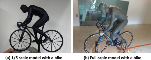
Figure 1(a) and 1(b) shows the photos of a 1/5 scale model and a full-scale model at a dropped position for the water-channel and wind-tunnel experiments, respectively. The cyclist models were made by a 3-D printer, with the contour data provided by TTRI (Taiwan Textile Research Institute). For the water-channel experiments, a bike model was made by the same 3-D printer to fit the 1/5 scale cyclist model, whereas for the wind-tunnel experiments a commercial bike was selected for the full-scale model. It is worthwhile to mention that the full-scale model was too large to be printed in one piece. Actually, it was segmented into 23 pieces for printing, then assembled afterwards.

Figure 1. The photos of (a) a 1/5 scale model with a bike for the water-channel experiment and (b) a full-scale model with a bike for the wind-tunnel experiment.

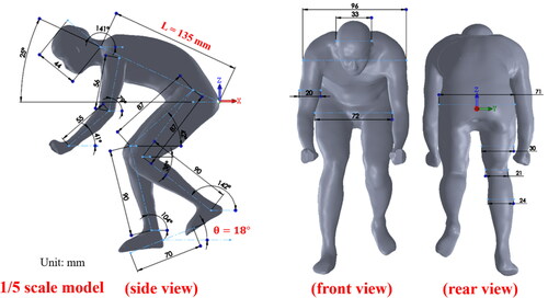
Detailed dimensions of a 1/5 scale cyclist model are shown in Figure 2. Notably, its pitch angle is 25^°, which is defined as the angle between the torso of the model indicated and the horizontal axis aligned in the direction of the incoming flow. The torso length, L, is denoted as the characteristic length in this study; L = 135 mm for the 1/5 scale model. Moreover, the coordinate system employed for this study is indicated in the figure with the origin located at the surface of the pelvis region, where x, y and z denote the streamwise, lateral and vertical directions, respectively.

Figure 2. Detailed dimensions of the 1/5 scale model with the coordinate system defined for this study.

Methods for the water-channel experiments

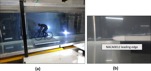
A closed-return type water channel was employed for the flow visualization experiments, with a test section of 0.6 m by 0.6 m in cross section and 2.5 m in length. The cyclist model was situated 1 m downstream from the inlet of the test section, where the turbulence intensity measured was about 1% of the incoming flow velocity at 0.09 m/s. As shown in Figure 3(a), the cyclist model and the bike were situated on a supporting plate, with a blockage ratio of 6.8% in total. Care was taken prior to the experiments to verify that the disturbance introduced by the ground plate had little effect on the flow downstream. This was confirmed by the dye-streak visualization image shown in Figure 3(b), unveiling that the disturbance produced from the leading edge had little impact on the flow downstream.

Figure 3. (a) A photo taken for the test section of the water channel. (b) A dye streak introduced upstream in the test section proving that flow over the leading edge of the ground plate did not produce additional disturbance.

Flow visualization experiments were performed using the dye-streak, oil-film and ink-dot methods. For the dye-streak method, the dye was introduced upstream from the model to reveal the flow motions in the region of interest. The outer diameter of the dye injection tube was 1 mm, that the Reynolds number based on the freestream velocity and the diameter of the tube was about 60. Note that the disturbance generated by the injection tube resulted in a wake behind the tube. Under the flow condition, the disturbance generated is categorized as a laminar wake (Roshko, 1954; Van Dyke, 1982), whose velocity deficit would be diffused by the viscous effect mainly. Thus, the disturbance produced could be regarded as insignificant to flow motion. For the oil-film method, a white water-color paint was applied on the surface of the model. After the model was placed in the flow for a length of time until most of the paint material on the windward side of the model was carried away, the flow separation lines would be revealed clearly. As for the ink-dot flow visualization technique, the same water-color paint was applied on the model surface in dots at the pre-determined grid points. Until the dotted paint dried for a certain length of time in the air, the model was placed in the test section. As a result, a limiting streamline pattern would be emerged from the appearance of the ink-dots due to the viscous effect of flow near the surface.

Methods for the wind-tunnel experiments

The ABRI (Architecture and Building Research Institute) wind tunnel (Miau et al., 2013) at the NCKU Kuei-Ren campus was employed for the present study. The wind tunnel is equipped with two test sections, including a primary test section which is 2.6 m by 4 m in cross section at the inlet and 36.5 m long, and the other which is 2.6 m by 6 m in cross section at the inlet and 21 m long. Driven by an axial fan with a motor rated 450 kW, the maximum speed in the primary test section could reach 36 m/s. At 2.5 m downstream from the inlet of the primary test section, where the cyclist model was situated, the non-uniformity of the flow was verified less than 0.4% of the free stream velocity (Kao, 2005; Miau et al., 2013). In the same cross-sectional plane, the free stream turbulence intensity measured by a single normal hot-wire probe was about 0.35% for the free stream velocities at 10 and 20 m/s, respectively. The thickness of the boundary layer developed on the floor at this streamwise location was about 60 mm at the free stream velocity 10 m/s.

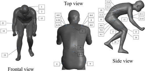
Experiments were carried out for the full-scale cyclist model shown in Figure 1(b), on which 32 pressure taps out of 75 in total were selected for measurements. See Figure 4 for the locations of the pressure taps selected. Each pressure tap was connected to a pressure sensor, AMS-5812-000-D-B, Analog Microelectronics GmbH, featuring a maximum frequency response of 500 Hz. Prior to the experiment, calibration was made for each of the sensors to obtain a relation between the output voltages and the known pressures, which were provided by a Druck DPI-610 portable pressure calibrator.

Figure 4. Indications of 32 pressure taps on the model surface with the frontal, top and side views.

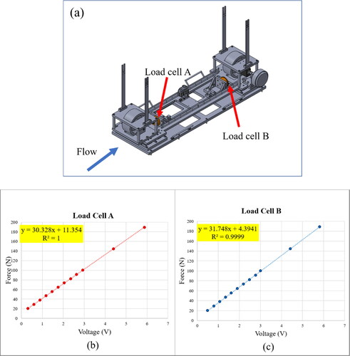
For the experiment, a self-made force balance system was employed to obtain the aerodynamic drag of the full-scale model together with the bike, with an area blockage ratio of 4.2% in total. In this study, no correction was made on the drag force measured with regard to the area blockage effect. The balance was designed to measure a one-component force in the streamwise direction. As shown in Figure 5(a), it was equipped with two S-Beam load cells, CLB-200NA, Tokyo Measuring Instruments Lab., which were installed in opposite directions to account for the forces in both directions. Calibration for each of the load cells was made prior to the wind-tunnel experiments. Figure 5(b) and 5(c) shows the calibration curves of the two load cells, respectively. For each of the load cells, the linearity of calibration could be examined by the correlation coefficient enclosed.

Figure 5. (a) A schematic view of the self-made force balance, (b) the calibration results of load cell A, and (c) the calibration results of load cell B.

In the wind tunnel, a Pitot tube was situated at the inlet of the test section to measure the free stream velocity, V_ref, which is denoted as the reference velocity for experiment. It was reduced from the output of a differential pressure transducer, Validyne DP-103, calibrated with the Druck DPI-610 portable pressure calibrator mentioned above. A thermometer was installed in the test section to monitor the temperature of the flow. For each set of the measurements, the output signals from the 32 pressure transducers, the force balance, the differential pressure transducer with the Pitot tube and the thermometer were sampled simultaneously by the analog to digital converter modules, NI-9215, at a rate of 1 kHz per channel for 120 s.

Design of textile roughness

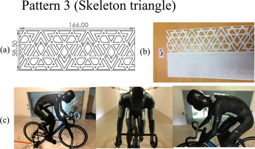
The sport suits tested in the wind tunnel experiments were made of different types of textile materials with addition of local roughness patterns. In an earlier study, Chen et al. (2019) demonstrated that applying a local roughness pattern on the cyclist model without textile material could have significant impact on drag reduction. The idea was that if a roughness pattern could be placed on the model surface at a location appropriate to disturbing the boundary-layer flow effectively, then the delay of flow separation would be remarkable. Chen et al. (2019) compared the results of ten different roughness patterns and found that a pattern called the skeleton triangle, which is shown in Figure 6, was the most effective for drag reduction. In Chen et al. (2019), the roughness patterns were applied on the shoulders, the upper arms, two sides of the waist and the outer sides of the upper legs at locations upstream, but close to, the flow separation lines as learned from the flow visualization experiments in the water channel. The thickness of each of the roughness patterns was 1 mm. A maximum reduction amounted to 6.7% was found in comparison with the drag coefficient of the model without a roughness pattern at the same Reynolds number. The Reynolds number is defined as Re= V_refL/ν; ν denotes the kinematic viscosity.

Figure 6. Illustrations of the roughness pattern called skeleton triangle (Chen et al., 2019). (a) The design drawing, (b) a view of the roughness pattern made of emulsion, and (c) the patterns applied on the shoulders, arms, waist and upper legs of the cyclist model (Chen et al., 2019).

The skeleton triangular pattern proposed by Chen et al. (2019) was implemented in the design of sport suits in this study. Seven sport suits were made for tests. See Figure 7 for the photos of the sport suits, named Cases 1R, 2R, 2RT, 3R, 3RT, 4R and 4RT. The characteristic features of the sport suits1R, 2R, 2RT, 3R and 3RT are further described in Table 1, which were made of four types of textile materials, named Types A, B, C and D. On the other hand, the textile materials of sport suits 4R, 4RT are identical and uniform in roughness, as described in Table 2.

Figure 7. The photos of the sport suits for the seven cases: Cases 1R, 2R, 2RT, 3R, 3RT, 4R and 4RT. Note that the characteristics of the sport suits are also described in Tables 1 and 2.

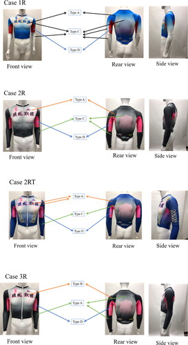
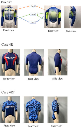
Table 1. Characteristics of the sport suits 1R, 2R, 2RT, 3R and 3RT, each of which was made of a combination of different types of textile materials as indicated.

(a) The textile materials used in the sport suits
Fabric type	Weight (gsm)	Fiber content	Fiber structural	Relative roughness (S10z/L)	Remarks
Type A	130	86% polyester 14% elastane	Warp knitting	5.88 × 10^−4	Uniform roughness
Type B	180	82% polyester 18% elastane	Warp knitting	α: 9.24 × 10^−4 β: 7.24 × 10^−4 (See Figure 8a for the sampled areas α and β)	Non-uniform roughness
Type C	150	80% polyester 20% elastane	Warp knitting	α: 9.04 × 10^−4 β: 5.6 × 10^−4 (See Figure 8b for the sampled areas α and β)	Non-uniform roughness
Type D	110	94% polyester 6% elastane	Warp knitting	α: 7.61 × 10^−4 β: 6.12 × 10^−4 (See Figure 8c for the sampled areas α and β)	Non-uniform roughness
(b) Descriptions of the design of the sport suits (See also Figure 7)
Case	Areas of the model surface with different fabric types				Local roughness pattern
	Front of the upper body	Shoulders and outer side of upper arms	Rear of the upper body	Inner side of the upper arms and the two sides of the upper body
1R	A	C	C	D	None
2R	A	A	C	D	None
2RT	A	A	C	D	Yes (2.45 mm thick)
3R	B	B	A	D	None
3RT	B	B	A	D	Yes (1.85 mm thick)

Table 2. Characteristics of sport suits 4R and 4RT, whose base textile materials were identical and uniform in roughness.

Case	Weight (gsm)	Fiber content	Yarn number	Fiber structure	Relative roughness (S10z/L)	Local roughness pattern
4R	200	Nylon/Spandex = 80/20	Nylon: 40 D; Spandex: 40 D	Warp knitting	5.56 × 10^−4	none
4RT	200	Nylon/Spandex = 80/20	Nylon: 40 D; Spandex: 40 D	Warp knitting	5.56 × 10^−4	Yes (0.5 mm thick)

Roughness of the textile materials is deemed critical to modify the boundary-layer flow on the model surface. Roughness measurements of the textile materials were carried out with a VK-9710 3 D laser scanning confocal microscope. Each image obtained was reduced for a quantity named S10z (ISO 25178, 2012), according to the definition below. (1) $$S10z=S5p+S5v$$(1) where S5p and S5v are the average heights of the five highest peaks and the deepest valleys, respectively, within an area of 1.5 mm by 1 mm measured. The relative roughness given in Tables 1 and 2 is defined as the S10z value normalized by the reference length, L = 0.675 m, the torso length of the full-scale model.

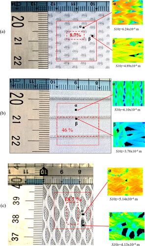
As indicated in Table 1, the textile materials of Types B, C and D are non-uniform in roughness. Details about the roughness patterns are further shown in Figure 8. Notably, for each of the types, the non-uniform roughness can be highlighted by the roughness measurements in two selected regions, named α and β, which are characterized by different textures. Moreover, in each of the photos, a dashed-line area marks a repeated pattern of the non-uniform roughness. A ratio of this area to a square of 20 mm by 20 mm indicated by the solid line is provided for reference.

Figure 8. The non-uniform textile materials of (a) Type B, (b) Type C and (c) Type D shown in Table 1. In each photo, α and β indicate the regions where the roughness measurements were made. The laser scanning images of the measurements corresponding to the two regions are enclosed. The percentage value indicated in each of the photos is the ratio of the area enclosed by the dashed line characterizing the repeated pattern of roughness versus the area enclosed by the solid line, 20 mm by 20 mm.

For Cases 2RT, 3RT and 4RT, the skeleton triangle patterns (Chen et al., 2019) were implemented. The thicknesses of the patterns varied in different cases, with the thicknesses of 2.45 mm, 1.85 mm and 0.5 mm for Cases 2RT, 3RT and 4RT, respectively. In addition, a case named Case O denoting the model without a sport suit was studied. The results of Case O will be referenced for comparison later.

Statistical analysis of the experimental data

In this study, the data sampled within a length of time for analysis, named a sampled record, is treated as a stationary random process (Bendat & Piersol, 1991). The methods of data analysis are presented below. The force-balance data obtained from a wind tunnel experiment can be reduced to the quantities of time-mean value $\overline{F}$ and root-mean square value F_rms, respectively. See the expressions below. (2) $$\overline{F}=\frac{1}{N}\sum _{i=1}^{N}F\mathrm{ }\left(i\right)$$(2) (3) $${\mathrm{F}}_{\text{rms}}=\sqrt{\frac{1}{N-1}{\sum _{i=1}^N(F-\overline{F})}^2}$$(3)

F(i): the real-time force value at the data point i sampled; N: the number of the data points in a sampled record, N = 12000.

Subsequently, the drag coefficient, C_D, and its root-mean square value, C_Drms, can be reduced according to the expressions below. (4) $$C_D=\frac{\overline{F}}{\frac{1}{2}{\mathrm{\rho }}_{\text{air}}{{\mathrm{V}}_{\text{ref}}}^2{\mathrm{A}}_{\mathrm{t}}}$$(4) (5) $$C_{D_{\mathit{rms}}}=\frac{{\mathrm{F}}_{\text{rms}}}{\frac{1}{2}{\mathrm{\rho }}_{\text{air}}{{\mathrm{V}}_{\text{ref}}}^2{\mathrm{A}}_{\mathrm{t}}}$$(5)

In the expressions above, ρ_air denotes the density of the air; A_t denotes the frontal area of the cyclist model together with the bike, 0.438 m².

Similarly, the pressure data obtained at each of the pressure taps on the model surface in a wind tunnel experiment can be reduced to the time-mean value $\overline{P}$ and the root-mean square value P_rms, respectively. See the expressions below. (6) $$\overline{P}=\frac{1}{N}\sum _{i=1}^{N}P\mathrm{ }\left(i\right)$$(6) (7) $${\mathrm{P}}_{\text{rms}}=\sqrt{\frac{1}{N-1}{\sum _{i=1}^N(P-\overline{P})}^2}$$(7)

P(i) denotes the real-time pressure value at the data point i sampled.

Subsequently, the pressure coefficient, C_p, and its root-mean square value, C_Prms, can be reduced according to the expressions below. (8) $$C_P=\frac{\overline{P}-P_{\mathit{static}}}{\frac{1}{2}{\mathrm{\rho }}_{\text{air}}{{\mathrm{V}}_{\text{ref}}}^2}$$(8) (9) $$C_{P_{\mathit{rms}}}=\frac{{\mathrm{P}}_{\text{rms}}}{\frac{1}{2}{\mathrm{\rho }}_{\text{air}}{{\mathrm{V}}_{\text{ref}}}^2}$$(9)

In the expressions above, P_static denotes the static pressure of the freestream flow. In addition, a real-time pressure coefficient, C_pr, is defined below. (10) $$C_{Pr}\left(i\right)=\frac{P\left(i\right)-P_{\mathit{static}}}{\frac{1}{2}{\mathrm{\rho }}_{\text{air}}{{\mathrm{V}}_{\text{ref}}}^2}$$(10)

CFD method for flow simulation

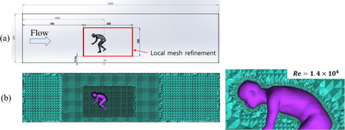
Numerical simulation of flow around the cyclist model without a bike was made to examine the phenomenon of flow separation from the body surface. A commercial software ANSYS Fluent was employed to solve the RANS (Reynolds-Averaged Navier-Stokes) equations using the SIMPLE algorithm. In solving the equations, a k-ω SST (Shear-Stress Transport) turbulence model was adopted. See Figure 9(a) for the computation domain. The dimensions were defined according to the test section of the water channel. A 1/5 scale cyclist model with no bike was situated in the domain. An adaptive grid system generated by the ANSYS ICEM software was employed, which consisted of seven million cells. The grid system is illustrated in Figure 9(b). Care was taken with the mesh size near the model to ensure that the distance from the first grid point to the surface of the body, in terms of y⁺, a non-dimensional distance based on the wall-friction velocity (White, 1974) and the kinematic viscosity, be less than 1. For the computation made at Re= 1.4 × 10⁴, the height of the first cell from the surface was 1.5 × 10⁻⁴ m. More information regarding the present computation method can be found in Tseng (2019).

Figure 9. The setup for the numerical simulation at Re = 1.4 × 10⁴. (a) The computation domain for simulating the flow over a 1/5 scale cyclist model in the test section of the water channel. (b) An illustration of the adaptive grid system employed for the numerical simulation.

Results and discussion

Results of the water-channel experiments

The results of flow visualization of the 1/5 scale model obtained in the water channel at Re = 1.4 × 10⁴ together with the CFD results obtained at the same Reynolds number are shown in Figure 10. Note that the flow visualization experiments were made for the model together with a sting support and a ground plate on the floor of the test section. On the other hand, the CFD simulation was carried out for the model only, for the sake of simplicity.

Figure 10. (a) Oil-film visualization on the back surface of the model; (b) an illustration of the counter-rotating vertical flows over the back of the model (Miau et al., 2020); (c) the wall shear-stress distribution on the back surface obtained by the present numerical simulation; (d) the ink-dot flow visualization on the back surface; (e) the skin friction distribution on the back surface; (f) and (g) the dye visualization of flow around the head of the model, respectively.

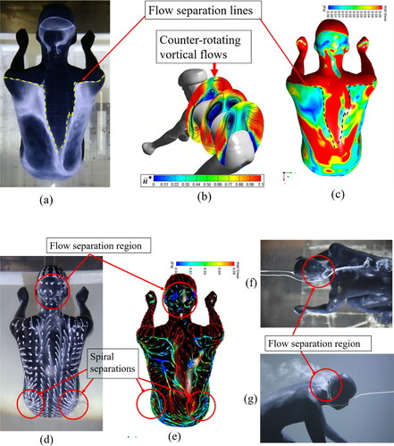
In Figure 10(a), the oil-film flow visualization results unveil the formation of the flow separation lines on the rear side of the shoulders, which were extended toward the center of the back of the model. This appearance is associated with two large-scale counter-rotating vortical flows induced by flow separation from the shoulders and the upper body, subsequently re-attached at the center of the back surface. For reference, a numerical plot of the streamline distribution in Figure 10(b) (Miau et al., 2020) for a cyclist model at the hoods position illustrates the formation of the vortical flows over the back surface. This flow characteristic was also mentioned in Crouch et al. (2014) and Crouch et al. (2017) for models at different postures. Figure 10(c) shows the numerical results of the wall shear stress distribution on the back surface of the present model. In this plot, the separation lines can be clearly discerned. Basically, the flow separation lines revealed from the shear stress distribution are conformed with those seen in the experimental flow visualization indicated by dashed lines in the numerical image. This comparison gives a strong support to the present numerical method, which is capable of unveiling the major flow characteristics around the cyclist model.

More details concerning the formation of the separation lines can be seen with the ink-dot visualization image and the corresponding numerical results shown in Figure 10(d) and 10(e), respectively. Both images clearly indicate that the formation of a flow separation line is resulted from a convergence of the limiting streamlines nearby. Physically, by the law of conservation of mass, a separation line is formed due to the convergence of the surrounding fluid near the surface, leading to a lift of the fluid from the surface (Lighthill, 1963). Furthermore, the complicated flow separation patterns revealed are attributed to the contoured surface of the model. Apart from the separation lines identified on the back of the model, two spiral separations formed on the two sides of the pelvis are noted in the figure. Each of the spiral separations is associated with the convergence of the limiting streamlines to a focal point, followed by a lift of the fluid from the focal point (Lighthill, 1963).

A flow separation region appeared on the rear side of the head of the model caught our attention, which can be further elaborated with the photos in Figure 10(f) and 10(g). The photo in Figure 10(f) was taken from a top view of the model with the dye streaks released upstream from the model. As seen, the flow around the head surface was entrained into a wake region, which was extended over the rear side of the head and the neck region. A side view shown in Figure 10(g) further indicates that a reversed flow was developed from the neck towards the head, subsequently shedding downstream. In accordance with the appearance of the diffused dye behind the head, one could further make an estimation about the lateral extent of the wake region.

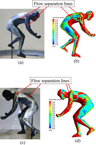
As a counterpart of Figure 10, Figure 11 presents the results of flow visualization obtained from the right and left sides of the cyclist model together with the CFD simulation results. The dashed lines marked in the photos indicate the flow separation lines identified by the flow visualization, which can be referenced for comparison. Two interesting aspects of the flow characteristics learned from the experimental and numerical results are described below. First, the flow separation lines along the two sides of the waist and the outer sides of the two legs basically follow the topology of the three-dimensional contoured surface as the cyclist model is facing the incoming flow. Second, the appearances of the flow separations lines on the upper right and left arms bear a similarity to a situation of flow over a normal circular cylinder. This observation strongly infers that flows around the upper arms can be modeled by flow over a circular cylinder, which will be elaborated later.

Figure 11. (a) Oil-film visualization on the right side of the model; (b) wall shear-stress distribution by numerical simulation on the right side of the model; (c) oil-film visualization on the left side of the model; (b) wall shear-stress distribution obtained by numerical simulation on the left side of the model.

Above findings enlighten an important aspect in sport suit design. Namely, if a sport suit with a roughness element could have significant impact on delaying the flow separation lines on the model, the reduction of drag would be remarkable. Accordingly, the sport suits of Cases 2RT and 3RT were designed with the skeleton triangle patterns (Chen et al., 2019) on the shoulders, waist and arms, whereas the Case 4RT was designed with the skeleton triangle patterns on the shoulders and arms. See also Figure 7 for the locations of the roughness patterns on the sport suits.

Results of the wind-tunnel experiments

The C_D distributions versus Re for all the eight cases studied in the wind-tunnel experiment are presented in Figure 12(a). Note that for each of the C_D values plotted, the accompanied error bars indicate the range of uncertainty. Owing to that at each of the flow speeds measured multiple measurements were made, the C_D value shown actually is the mean of the repeated measurements, whereas the upper and lower error bars indicate the highest and lowest C_D values obtained, respectively. As a counterpart of the plot of the C_D distributions, a plot of the distributions of C_Drms, i.e., the standard deviation associated with the C_D values, is given in Figure 12(b). Similarly, each of the C_Drms value plotted correspond to the mean of multiple measurements, accompanied with the error bars to indicate the range of the C_Drms values among the measurements.

Figure 12. The distributions of C_D and C_Drms versus Re for all the cases studied. The C_D and C_Drms distribution of Case 3R are highlighted with solid symbols.

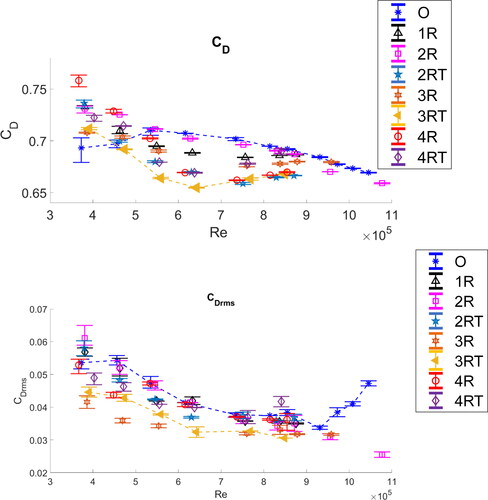
For Case O, the C_D values are the highest compared to the seven cases with the sport suits for the Reynolds numbers higher than 5.5 × 10⁵. As noted, at Re = 3.9 × 10⁵ the uncertainty associated with the plotted value was pronouncedly higher than those at higher Reynolds numbers due to the contamination of background noise in the measured signals. For Case O, Re= 5.5 × 10⁵ to 10 × 10⁵, the C_D values appear to decrease monotonically with Re, from 0.71 to 0.67. On the other hand, the C_Drms distribution of Case O shows a trend of decreasing with Re up to 9 × 10⁵, but reversed the trend at higher Re. This infers that the flow unsteadiness gets more pronounced at Re beyond 9 × 10⁵.

Discussion on the C_D data of the seven cases with sport suits is made below. Comparing the C_D distributions of Cases 1R and 2R, whose sport suits feature different materials at the shoulders but identical in other areas, the difference is rather significant. Namely, the C_D distribution of Case 1R shows a significant reduction compared to that of Case O for Re higher than 5.5 × 10⁵. On the other hand, the distribution of Case 2R appears to be similar to that of Case O with small differences only. In fact, the distribution of Case 2R is the only one among the seven cases with sport suits that shows no appreciable reduction in drag for Re higher than 5.5 × 10⁵. Based on this finding, one can say that the surface roughness at the shoulders plays a critical role to reduce drag at high Reynolds numbers, and in Case 2R the textile material at the shoulders could be too smooth to have a significant impact on delaying flow separation.

A comparison of the C_D distributions of Cases 2R and 2RT, whose textile materials are identical, unveils that the latter with the skeleton triangular patterns implemented has a significant impact on drag reduction. In the C_D distribution of 2RT, a minimum C_D value can be identified at Re between 7 × 10⁵ and 8 × 10⁵, beyond which the C_D value gets increased. This appearance infers the existence of a critical condition under which the C_D value reaches a minimum. The corresponding Reynolds number can be named as the critical Reynolds number (Hsu et al., 2019). A similar finding was pointed out by Basu (1985) in reviewing the experimental results of flows over roughened two-dimensional circular cylinders. Physically speaking, the critical flow phenomenon in flow over a two-dimensional circular cylinder is accompanied with the formation of separation bubbles on the circular cylinder (Zdravkovich, 1997; Bearman, 1969). Likewise, one would expect that separation bubbles could be formed on the surface of the cyclist model, although the model is much more complicated in a 3-D contoured shape. More findings in this regard will be presented later.

Cases 3R and 3RT feature sport suits with the same textile materials, but the latter includes the skeleton triangular patterns. A comparison of the C_D distributions of the two cases reveals a difference similar to that seen in Cases 2R and 2RT that the artificial roughness pattern has a positive impact on drag reduction, even though the thickness of the roughness pattern of Case 3RT is less than that of Case 2RT. Meanwhile, it is worthwhile to mention that the critical C_D value obtained in Case 3RT appears to be the lowest among all the cases presented in the figure. Note that in Figure 12(a), the C_D distribution of Case 3RT is highlighted with solid symbols. In this case, the critical condition occurred about Re= 6.4 × 10⁵, which is lower than the critical Reynolds number in Case 2RT mentioned above. Referring to the C_D value of Case O at the same Reynolds number, the reduction in Case 3RT is amounted to 7.5%.

Comparing the C_D distributions of Cases 4R and 4RT, it is found that the addition of the skeleton triangular patterns at the shoulders and arms in fact has a negative impact on drag reduction at Reynolds numbers beyond the critical value about 6 × 10⁵. Evidently, this finding is contrary to that learned from Cases 2R, 2RT, 3R and 3RT above. In summary, the comparisons made above suggest that the effectiveness of the local roughness patterns deserves careful investigation for each of the individual cases.

To better understand the physical mechanism of surface roughness involved in drag reduction, it is worthwhile to examine the pressure data obtained on the model surface. In the following, the results of the pressure measurements made on the shoulders, the right waist and the right arm are presented for discussion. Similar to Figure 12, each of the C_p or C_prms values plotted in the following figures is the mean of the values obtained from multiple measurements, accompanied with the error bars to indicate the range of variations among the measurements.

Figures 13 and 14 present the distributions of C_p and C_prms on the right and left shoulders, respectively, versus Reynolds number for all the cases studied. The locations of the pressure taps on the right shoulder, named 4-4, 4 and 4-6, and on the left shoulders, named 4-8, 4-10 and 4-14, are shown in the figures for reference.

Figure 13. (a) $C_p\mathrm{ }$ and (b) $C_{\mathit{prms}}$ distributions versus Re at pressure taps 4-4, 4 and 4-6 on the right shoulder of the model for all cases studied. The C_p and $C_{\mathit{prms}}$ distributions of Cases 1R and 2RT are highlighted with solid symbols, which are connected by dashed lines respectively. In each of the plots, the distribution of Case O is plotted with a dashed line for reference.

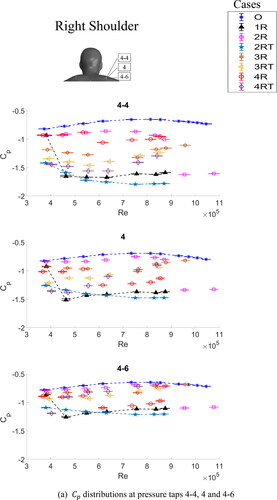
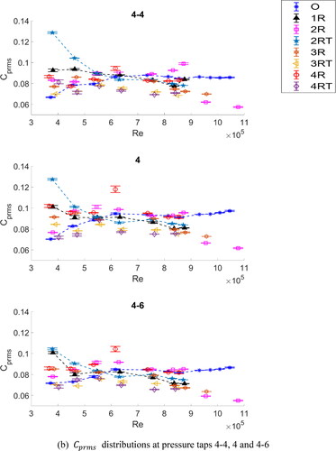
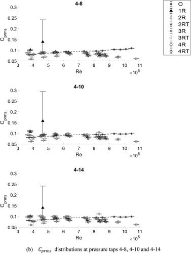
Figure 14. (a) $C_p\mathrm{ }$ and (b) $C_{\mathit{prms}}$ distributions versus Re at pressure taps 4-8, 4-10 and 4-14 on the left shoulder of the model for all cases studied. The C_p distributions of Cases 1R and 2RT are highlighted with solid symbols, which are connected by dashed lines respectively. The C_prms distributions of Case 1R in the three plots of (b) are highlighted with solid symbols. In each of the plots, the distribution of Case O is plotted with a dashed line for reference.

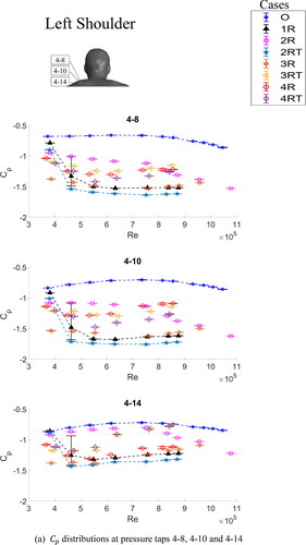
In comparing the C_p distributions of all the eight cases, one finds a feature in common in the two figures that the distributions of Case O show the least negative. In viewing that flow separations were developed on both shoulders (Figure 10), this appearance infers that for all the seven cases with sport suits the flow separations on the shoulders were actually delayed downstream relative to the Case O. Further explanation in this regard can be made below. Delay of flow separation on the upper surface of a shoulder is equivalent to a situation that the boundary-layer flow persists over the shoulder surface a longer distance, which basically is convex in shape. Thus, the attached flow keeps accelerating along the surface, leading to lower static pressure at the pressure taps measured. Based on this reasoning, one can further argue that among the seven cases with sport suits Cases 1R and 2RT appear to be the most effective in delaying the flow separation over the shoulders, as the C_p values show the most negative. In the figures, the C_p distributions of the two cases are highlighted with solid symbols.

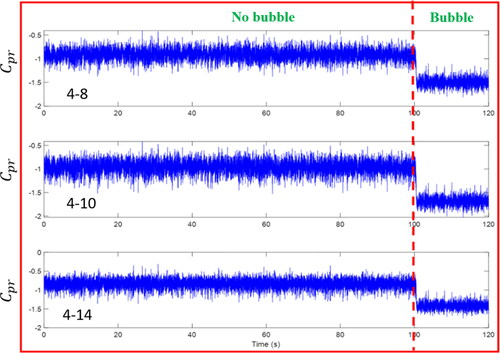
The value of C_prms basically indicates the degree of flow unsteadiness at the pressure tap measured. Presumably, the flow unsteadiness is predominated by flow separation on the shoulders, a situation like flow over a circular cylinder where the flow unsteadiness is mainly associated with the phenomenon of vortex shedding (Bloor, 1964; Gerrard, 1966; Miau et al., 2006). In Figures 13 and 14, it is noted that for all the cases studied, the C_prms values are about 0.1 in general. This observation infers that the unsteadiness of flow over both shoulders was not affected by the sport suits appreciably. Nevertheless, special attention is paid to Case 1R at Re= 4.6 × 10⁵ in Figure 14(b), where the C_prms values at the three pressure taps 4-8, 4-10 and 4-14 on the left shoulder appear distinctly higher. The distributions of Case 1R in the three plots of Figure 14(b) are highlighted with solid symbols. To gain further insights into this finding, the real-time pressure coefficient traces in terms of C_pr are presented in Figure 15 for examination. In the figure, the three real-time traces consistently indicate an abrupt change from −1 to −1.5 at t = 100 s. Physically, this appearance infers that a separation bubble was formed on the left shoulder at the time instant and remained afterwards. The formation of a separation bubble on the shoulder would alter the pressure distribution remarkably, as evidenced in flow over a circular cylinder in the critical regime (Farell & Blessman, 1983; Gaster, 1969; Lin et al., 2011; Miau et al., 2011; Tani, 1964).

Figure 15. The real-time C_pr traces obtained at three pressure taps, 4-8, 4-10 and 4-14, of Case 1R at Re= 4.6 × 10⁵. All three traces consistently indicate that at the time instant 100 s, the laminar separation bubble is formed on the left shoulder.

More discussions on the C_p distributions of Cases 1R and 2RT in Figures 13(a) and 14(a) can be made below. In Figure 13(a), it is noticed that the C_p distributions of Case 1R at the pressure taps 4-4, 4 and 4-6 consistently show a significant drop at Re= 4.6 × 10⁵. Similar finding is noted in Figure 14(a) for the C_p distributions of Cases 1R and 2RT at the pressure taps 4-8, 4-10 and 4-14. Remarkable uncertainties associated with the C_p values of Case 1R at Re= 4.6 × 10⁵ in all the plots in Figure 14(a) as well as the corresponding C_prms plots in Figure 14(b) infer the unsteadiness of the formation of separation bubble. The effect of delaying flow separation is seen at this Reynolds number and beyond. For Case 2RT, in viewing that the roughness elements situated on the windward side of both shoulders (Figure 7), the boundary layer flows on the shoulders were tripped to promote turbulent momentum mixing, thus delay flow separation effectively.

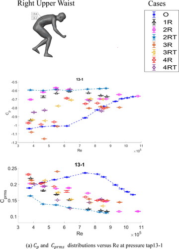
Discussion on the characteristics of the separated flow around the right waist of the cyclist model can be made by examining the C_p and C_prms data obtained at pressure taps 13-1 and 13-6. For all the eight cases studied, the distributions of C_p and C_prms versus Re are presented in Figure 16 for comparison. Several interesting features of the flow characteristics deserve attention here. First, on the pressure data obtained at the pressure tap 13-1, the C_p values of Case O show a trend of increasing with Re up to 10 × 10⁵, and the corresponding C_prms values maintain at a relatively high level compared to the rest cases, and reach a peak around Re= 7 × 10⁵. These observations suggest that for Case O, flow separation around the waist is accompanied with strong flow unsteadiness, which gets less significant at Re beyond 7 × 10⁵. Since the separated flow developed from the waist is merged into the wake flow behind the back of the cyclist model, the appearance of high C_prms values could be intimately associated with the flow unsteadiness of the wake flow behind the back of the model. Based on this reasoning, one could further argue that since the C_prms values show a trend of decreasing with Re, the flow unsteadiness associated with the wake gets less severe as Re increased beyond 7 × 10⁵. For the seven cases with sport suits, the C_p distributions show less variations with Re and the C_prms distributions stay at lower values compared to that of Case O. These findings infer that the wake flow behind the back of the cyclist model tends to be reduced in size with less unsteadiness, compared to Case O. Examining the data in the figure, one may further obtain an idea that the most remarkable change is due to Case 2RT, whose C_p and C_prms distributions at the pressure tap 13-1 are highlighted with the solid symbols in Figure 16(a).

Figure 16. $C_p\mathrm{ }$ and (b) $C_{\mathit{prms}}$ distributions versus Re at pressure taps (a) 13-1 and (b) 13-6 on the upper right waist of the model for all the cases studied. The C_p and C_prms distributions of Case 2RT at the pressure tap 13-1 in (a) are highlighted with solid symbols, which are connected by dashed lines. The C_p and C_prms distributions of Case 2RT and 3RT at the pressure tap 13-6 in (b) are highlighted with solid symbols, which are connected by dashed lines. In each of the plots, the distribution of Case O is plotted with a dashed line for reference.

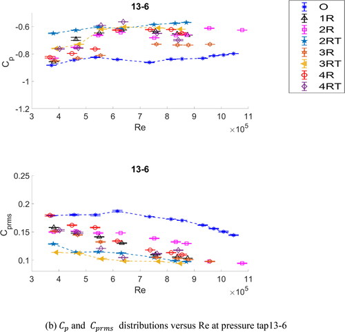
Second, at pressure tap 13-6, for each of the cases the C_p distribution versus Re appears to be almost constant. Meanwhile, the C_prms values stay low. These findings suggest that pressure tap 13-6 be located in the wake region. The C_p distribution of Case O appears to be the lowest in value among the eight cases studied, implying that the flow separation line in this case would be located farthest upstream compared to the other cases. This can be reasoned with our knowledge about flow around a bluff body. Delaying flow separation on a contoured surface would result in an increase in base pressure, such as in the case of flow over a circular cylinder (Achenbach, 1968; Igarashi, 1978; Roshko, 1993). Moreover, a numerical study by Phung et al. (2017) on flow over a cyclist model at the hoods position using a Large-Eddy-Simulation (LES) method indicated that the flow separation lines on the contoured surface of the waist region were actually wandering in time, and the drag coefficient in real time varied accordingly. Following this reasoning, one can argue that as far as delaying the flow separation around the waist region is concerned, Case 2RT or 3RT appears to be the most effective, accompanied with the least flow unsteadiness measured. Conceivably, the addition of the local roughness patterns at the waist in the two cases had a significant impact on the flow development. The C_p and C_prms distributions of the two cases corresponding to the pressure tap 13-6 are highlighted in Figure 16(b) with solid symbols. A summary based on above findings at two pressure taps suggests that Case 2RT is the most effective in delaying flow separation in the waist region of the model.

The C_p and C_prms data obtained at pressure taps 21, 22, 21-1 and 21-4 on the right arm of the cyclist model are presented in Figure 17 for discussion. Notably, the locations of pressure taps 21 and 22 are on the windward and rearward sides, respectively. Pressure taps 21-1 and 21-4 are located on the outer side of the arm where the flow separation phenomenon would be anticipated.

Figure 17. (a) $C_p\mathrm{ }$ and (b) $C_{\mathit{prms}}$ distributions versus Re at pressure taps 21, 22, 21-1 and 21-4 on the upper right arm of the model for all the cases studied. In the figure, the C_p and C_prms distributions of Case 2R are highlighted with solid symbols, which are connected by dashed lines; the C_p and C_prms distributions of Case 4R are highlighted with solid symbols. In each of the plots, the distribution of Case O is plotted with a dashed line for reference.

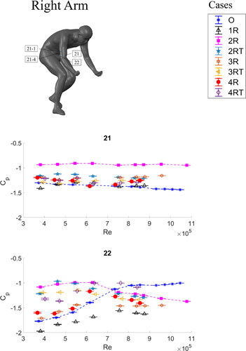
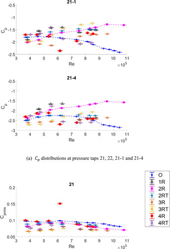
The C_p and C_prms data obtained at pressure tap 22 basically reflect the characteristics of flow in the wake region behind the arm. For Case O, the C_p values appear to be increased with Re and approach to a level about −1 for Re beyond 7 × 10⁵, meanwhile the C_prms values appear to be decreased remarkably for Re beyond 7 × 10⁵. These findings strongly suggest that flow separation be delayed further rearward as Re gets increased up to 7 × 10⁵. On the other hand, attention is drawn to Case 2R. The distribution of C_prms versus Re unveils a trend that the flow unsteadiness appears to be more severe than that of Case O at Re beyond 7 × 10⁵. Meanwhile, the C_p and C_prms distributions of Case 2R show no appreciable variations with Re, which infers no evidence about the occurrence of the critical transition phenomenon. This can be also learned from the C_p data obtained from pressure taps 21-1 and 21-4 that for Case 2R the C_p values stay about −1.5 for Re beyond 7 × 10⁵, which is attributed to no formation of separation bubble on the outer surface of the right arm. Also noted from the C_p distributions of the pressure tap 21 in the figure, the Case 2R appears to have the least negative values and remain almost constant, slightly less negative than −1, over the Reynolds number range studied. In the figure, the C_p and C_prms distributions of Case 2R are highlighted with the solid symbols.

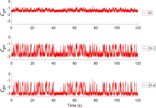
For Case 4R, the C_prms data obtained at Re= 6 × 10⁵, at pressure taps 21-1 and 21-4, show distinctly high values compared to those of the other cases. Interestingly, this phenomenon was confirmed by a repeated measurement. To gain better understanding on these data, the real-time C_pr traces of one set of the measurements at the two pressure taps are presented in Figure 18, in which the real-time trace at the pressure tap 21 is also included for reference. Notably, high C_prms values are attributed to pressure fluctuations with large amplitude characterized by two levels. The two levels in fact correspond to on and off, respectively, concerning the formation of a separation bubble on the arm surface. This has been seen in flow over a circular cylinder, for which switching between states appears to be very pronounced in the critical transition range (Bearman, 1969; Lin et al., 2011; Miau et al., 2011; Zdravkovich, 1997). To be more specific, in the real-time C_pr traces, the level of −3 infers the presence of a separation bubble on the arm surface. On the other hand, the pressure coefficient at the level of −1 infers no presence of a separation bubble. The large pressure fluctuations imply that the arm of the cyclist model would be experiencing a remarkably unsteady side force.

Figure 18. The real-time C_pr traces obtained at the three pressure taps, 21, 21-1 and 21-4, of Case 4R at Re= 6.2 × 10⁵. The traces obtained at pressure taps 21-1 and 21-4 show fluctuations between the levels of -1 and -3, inferring switching off and on regarding the formation of the separation bubble on the arm surface.

For Case 4R, the C_p distribution at pressure tap 21-1 appears to drop to the lowest value about −2.2 at Re= 6 × 10⁵, and then recovers to a less negative value about −1.6 at higher Re. Meanwhile, the C_p distribution at pressure tap 21-4 shows that it levels off at about −2.5 for Re= 6 × 10⁵ and beyond. These findings suggest that in this case the separation bubble stay on the arm surface for Re beyond 6 × 10⁵. The corresponding C_prms distributions appear to stay at low values in this Re range, implying that the separation bubble is stably situated on the arm. In the figure, the C_p and C_prms distributions of Case 4R are highlighted with solid symbols.

Conclusions

Fruitful results were obtained in this study, in terms of the flow visualization on a 1/5 scale model made in a water channel supplemented by the results of numerical simulation, and the drag force and pressure measurements made in a wind tunnel on a full-scale cyclist model with seven sport suits. These findings lead to the following conclusions.

1. The C_D data of six out of the seven cases with sport suits clearly indicate that a critical condition with remarkable drag reduction can be reached within the Reynolds number range studied.

2. Comparing the C_D data obtained for the seven cases with sport suits indicates that both the base textile materials and the local roughness pattern are crucial to the reduction of aerodynamic drag. Evaluation on the effectiveness should be made for each of the individual cases, whereas no general guidelines could be recommended. The best result found in this study is due to the Case 3RT that the drag reduction is amounted to 7.5% at Re= 6.4 × 10⁵, compared to that of Case O.

3. By examining the C_p and C_prms data together with the C_D data obtained for all the cases studied, reduction of drag evidently is accompanied with the delay of flow separation on the model and lower the flow unsteadiness around the model.

4. The present findings of separation bubbles on the local surfaces of the cyclist model provide a directly support to the statement made in the literature (Brownlie et al., 2009) that the critical transition phenomenon could have a significant impact on drag reduction of the aerodynamic flow around a cyclist body.

Acknowledgements

The authors would like to express their sincere appreciation to Taiwan Textile Research Institute for providing the 3-D contour data of the cyclist model for this study and Architecture Building Research Institute for the technical assistance in the wind tunnel experiments. Sincere appreciation also goes to Mr. Tzu-Liang Chen who designed the force balance for the wind tunnel experiments. Funding support by Ministry of Science and Technology, Taiwan, under the project number: 108-2627-H-006-003 for this work is gratefully acknowledged.

Disclosure statement

No potential conflict of interest was reported by the authors.

References

- Achenbach, E. (1968). Distribution of local pressure and skin friction around a circular cylinder in cross-flow up to Re = 5 × 10⁶. Journal of Fluid Mechanics, 34(4), 625–639. https://doi.org/https://doi.org/10.1017/S0022112068002120
- Achenbach, E. (1971). Influence of surface roughness on the cross-flow around a circular cylinder. Journal of Fluid Mechanics, 46(2), 321–335. https://doi.org/https://doi.org/10.1017/S0022112071000569
- Basu, R. I. (1985). Aerodynamic forces on structures of circular cross-section. Part 1. Model-scale data obtained under two-dimensional conditions in low-turbulence streams. Journal of Wind Engineering and Industrial Aerodynamics, 21(3), 273–294. https://doi.org/https://doi.org/10.1016/0167-6105(85)90040-6
- Bearman, P. W. (1969). On vortex shedding from a circular cylinder in the critical regime. Journal of Fluid Mechanics, 37(3), 577–585. https://doi.org/https://doi.org/10.1017/S0022112069000735
- Bendat, J. S., & Piersol, A. G. (1991). Random data analysis and measurement procedures (2nd ed.). John Wiley & Sons.
- Blocken, B., Defraeye, T., Koninckx, E., Carmeliet, J., & Hespel, P. (2013). CFD simulations of the aerodynamic drag of two drafting cyclists. Computers & Fluids, 71, 435–445. https://doi.org/https://doi.org/10.1016/j.compfluid.2012.11.012
- Blocken, B., van Druenen, T., Toparlar, Y., & Andrianne, T. (2018a). Aerodynamic analysis of different cyclist hill descent positions. Journal of Wind Engineering and Industrial Aerodynamics, 181, 27–45. https://doi.org/https://doi.org/10.1016/j.jweia.2018.08.010
- Blocken, B., van Druenen, T., Toparlar, Y., Malizia, F., Mannion, P., Andrianne, T., Marchal, T., Maas, G.-J., & Diepens, J. (2018b). Aerodynamic drag in cycling pelotons: New insights by CFD simulation and wind tunnel testing. Journal of Wind Engineering and Industrial Aerodynamics, 179, 319–337. https://doi.org/https://doi.org/10.1016/j.jweia.2018.06.011
- Bloor, M. S. (1964). The transition to turbulence in the wake of a circular cylinder. Journal of Fluid Mechanics, 19(02), 290–304. https://doi.org/https://doi.org/10.1017/S0022112064000726
- Brownlie, L., Kyle, C., Carbo, J., Demarest, N., Harber, E., MacDonald, R., & Nordstrom, M. (2009). Streamlining the time trial apparel of cyclists: he Nike Swift Spin project. Sports Technology, 2(1–2), 53–60. https://doi.org/https://doi.org/10.1080/19346182.2009.9648499
- Chen, J. J., Miau, J. J., & Tseng, C. H. (2019). Flow over a complex bluff body: Investigation of flow visualization of the cyclist. 14th International Symposium on Advanced Science and Technology in Experimental Mechanics, 1–4 November, 2019, Tsukuba, Japan.
- Chowdhury, H., Alam, F., Mainwaring, D., Subic, A., Tate, M., Forster, D., & Beneyto-Ferre, J. (2009). Design and methodology for evaluating aerodynamic characteristics of sports textiles. Sports Technology, 2(3–4), 81–86. https://doi.org/https://doi.org/10.1080/19346182.2009.9648505
- Crouch, T. N., Burton, D., Brown, N. A. T., Thompson, M. C., & Sheridan, J. (2014). Flow topology in the wake of a cyclist and its effect on aerodynamic drag. Journal of Fluid Mechanics, 748, 5–35. https://doi.org/https://doi.org/10.1017/jfm.2013.678
- Crouch, T. N., Burton, D., LaBry, Z. A., & Blair, K. B. (2017). Riding against the wind: A review of competition cycling aerodynamics. Sports Engineering, 20(2), 81–110. https://doi.org/https://doi.org/10.1007/s12283-017-0234-1
- Crouch, T. N., Burton, D., Thompson, M. C., Brown, N. A., & Sheridan, J. (2016a). Dynamic leg-motion and its effect on the aerodynamic performance of cyclists. Journal of Fluids and Structures, 65, 121–137. https://doi.org/https://doi.org/10.1016/j.jfluidstructs.2016.05.007
- Crouch, T., Burton, D., Venning, J., Thompson, M., Brown, N., & Sheridan, J. (2016b). A comparison of the wake structures of scale and full-scale pedalling cycling models. Procedia Engineering, 147, 13–19. https://doi.org/https://doi.org/10.1016/j.proeng.2016.06.182
- Debraux, P., Grappe, F., Manolova, A. V., & Bertucci, W. (2011). Aerodynamic drag in cycling: Methods of assessment. Sports Biomechanics, 10(3), 197–218. https://doi.org/https://doi.org/10.1080/14763141.2011.592209
- Defraeye, T., Blocken, B., Koninckx, E., Hespel, P., & Carmeliet, J. (2010). Aerodynamic study of different cyclist positions: CFD analysis and full-scale wind-tunnel tests. Journal of Biomechanics, 43(7), 1262–1268. https://doi.org/https://doi.org/10.1016/j.jbiomech.2010.01.025
- Defraeye, T., Blocken, B., Koninckx, E., Hespel, P., & Carmeliet, J. (2011). Computational fluid dynamics analysis of drag and convective heat transfer of individual body segments for different cyclist positions. Journal of Biomechanics, 44(9), 1695–1701. https://doi.org/https://doi.org/10.1016/j.jbiomech.2011.03.035
- Defraeye, T., Blocken, B., Koninckx, E., Hespel, P., Verboven, P., Nicolai, B., & Carmeliet, J. (2014). Cyclist drag in team pursuit: Influence of cyclist sequence, stature, and arm spacing. Journal of Biomechanical Engineering, 136(1), 011005. https://doi.org/https://doi.org/10.1115/1.4025792
- Farell, C., & Blessman, J. (1983). On critical flow around smooth circular cylinders. Journal of Fluid Mechanics, 136(1), 375–391. https://doi.org/https://doi.org/10.1017/S0022112083002190
- Fintelman, D. M., Sterling, M., Hemida, H., & Li, F. X. (2014). Optimal cycling time trial position models: Aerodynamics versus power output and metabolic energy. Journal of Biomechanics, 47(8), 1894–1898. https://doi.org/https://doi.org/10.1016/j.jbiomech.2014.02.029
- Gaster, M. (1969). The structure and behavior of separation bubbles. No. 3595.
- Gerrard, J. H. (1966). The mechanics of the formation region of vortices behind bluff bodies. Journal of Fluid Mechanics, 25(2), 401–413. https://doi.org/https://doi.org/10.1017/S0022112066001721
- Hsu, X. Y., Miau, J. J., Tsai, J. H., Tsai, Z. X., Lai, Y. H., Ciou, Y. S., Shen, P. T., Chuang, P. C., & Wu, C. M. (2019). The aerodynamic roughness of textile materials. The Journal of the Textile Institute, 110(5), 771–779. https://doi.org/https://doi.org/10.1080/00405000.2018.1518636
- Igarashi, T. (1978). Flow characteristics around a circular cylinder with a slit. Bulletin of JSME, 21(154), 656–664. https://doi.org/https://doi.org/10.1299/jsme1958.21.656
- Kao, Y. M. (2005). Calibration of the ABRI environment wind tunnel and experimental study of 2-D bluff body aerodynamic flows [Master thesis]. Department of Aeronautics and Astronautics, National Cheng Kung University.
- Kyle, C. R., & Burke, E. (1984). Improving the racing bicycle. Mechanical Engineering, 106(9), 34–45.
- Lighthill, M. L. (1963). Introduction, boundary layer theory. In L. Rosenhead (Ed.), Laminar boundary layers (Chap. II). Oxford University Press.
- Lin, Y. J., Miau, J. J., Tu, J. K., & Tsai, H. W. (2011). Non-stationary, three-dimensional aspects of flow around a circular cylinder at critical Reynolds numbers. AIAA Journal, 49(9), 1857–1870. https://doi.org/https://doi.org/10.2514/1.J050674
- Miau, J. J., Chen, Z. L., & Hu, C. C. (2013). The characteristics of the ABRI wind tunnel. In S. B. Chaplin (Ed.), Wind tunnels: Design/construction, types and usage limitations (pp. 1–33). Nova Science Publishers.
- Miau, J. J., Li, S. R., Tsai, Z. X., Phung, M. V., & Lin, S. Y. (2020). On the aerodynamic flow around a cyclist model at the hoods position. Journal of Visualization, 22, 35–47.
- Miau, J. J., Tsai, H. W., Lin, Y. J., Tu, J. K., Fang, C. H., & Chen, M. (2011). Experiment on smooth circular cylinders in cross-flow in the critical Reynolds number regime. Experiments in Fluids, 51(4), 949–967. https://doi.org/https://doi.org/10.1007/s00348-011-1122-2
- Miau, J. J., Tu, J. K., Chou, J. H., & Lee, G. B. (2006). Sensing flow separation on a circular cylinder by MEMS thermal-film sensors. AIAA Journal, 44(10), 2224–2230. https://doi.org/https://doi.org/10.2514/1.17408
- Nakamura, Y., & Tomonari, Y. (1982). The effects of surface roughness on the flow past circular cylinders at high Reynolds numbers. Journal of Fluid Mechanics, 123, 363–378. https://doi.org/https://doi.org/10.1017/S0022112082003103
- Nikuradse, J. (1937). Laws of flow in rough pipes. NACA Technical Memorandum 1292.
- Oggiano, L., Saetran, L., Løset, S., & Winther, R. (2007). Reducing the athlete’s aerodynamic resistance. Journal of Computational and Applied Mechanics, 8(2), 163–173.
- Oggiano, L., Troynikov, O., Konopov, I., Subic, A., & Alam, F. (2009). Aerodynamic behavior of single sport jersey fabrics with different roughness and cover factors. Sports Engineering, 12(1), 1–16. https://doi.org/https://doi.org/10.1007/s12283-009-0029-0
- Phung, M. V., Miau, J. J., Lin, S. Y., & Li, S. R. (2017). A research of wake development in Cycling Hood Position. 12th International Symposium on Advanced Science and Technology in Experimental Mechanics, 1–4 November 2017, Kanazawa, Japan.
- Roshko, A. (1954). On the development of turbulent wakes from vortex streets. NACA Report, 1191.
- Roshko, A. (1993). Perspectives on bluff body aerodynamics. Journal of Wind Engineering and Industrial Aerodynamics, 49(1–3), 79–100. https://doi.org/https://doi.org/10.1016/0167-6105(93)90007-B
- Schewe, G. (1983). On the force fluctuations acting on a circular cylinder in cross flow from subcritical up to transcritical Reynolds numbers. Journal of Fluid Mechanics, 133, 265–283. https://doi.org/https://doi.org/10.1017/S0022112083001913
- Tani, I. (1964). Low-speed flows involving bubble separations. Progress in Aerospace Sciences, 5, 70–103. https://doi.org/https://doi.org/10.1016/0376-0421(64)90004-1
- Tseng, C. H. (2019). Research of the flow structure and experiment data on full and small scale cyclist model [Master thesis]. Department of Aeronautics and Astronautics, National Cheng Kung University.
- Van Dyke, M. (1982). An album of fluid motion. The Parabolic Press.
- White, F. M. (1974). Viscous fluid flow. McGraw-Hill, Inc.
- Wieselsberger, C. (1922). New data on the law of fluid resistance. NACA Technical Note, 84.
- Zdravkovich, M. M. (1997). Flow around circular cylinders: Fundamentals (Vol. 1, pp. 1–18). Oxford University Press.