Identification and analysis of fibers in ultra-large micro-CT scans of nonwoven textiles using deep learning

Abstract

Fibrous materials play a significant role in many industries, such as lightweight automotive materials, filtration, or as constituents of hygiene products. The properties of fibrous materials are governed to a large extent by their microstructure. One way to access the microstructure is to use micro-Computed Tomography (micro-CT). Completely characterizing the microstructure requires geometrically characterizing each individual fiber. To make this possible, one must identify the individual fibers. Our method achieves this by finding in segmented µCT scans the centerline of all individual fibers. It uses a convolutional neural network that was trained on automatically generated synthetic training data. From the centerlines, analytic descriptions of the individual fibers are constructed. These analytic representations allow detailed insights into the statistics of the geometric properties of the fibrous material, such as the fibers’ orientation, length, or curvature. The method is validated on artificial data sets and its usefulness demonstrated on a very large micro-CT scan of a nonwoven composed of long fibers with random curvature.

Keywords:

• Nonwovens
• deep learning
• micro-CT
• fiber identification

Introduction

Fibrous materials play a significant role in many industries, such as lightweight automotive materials (May et al., 2020), filtration (Hoess et al., 2021), or as constituents of hygiene products (Rigby et al., 1997). Because the details down to the individual fibers govern the material properties, understanding the microstructural geometric statistics of fibrous materials is an essential aspect of material engineering. Analyzing fibers have therefore been a research interest for a long time. First, besides manual measurements, 2 D image analysis was used for this task (Pourdeyhimi & Ramanathan, 1995).

In the last 15 years, volumetric 3 D scanning technology such as micro-CT has become affordable and widely available, popularizing its application for the analysis of nonwovens (Suragani Venu et al., 2012; Soltani et al., 2015). 3 D scans can provide valuable insights into materials under two constraints: The scanning resolution must be sufficient to resolve all relevant objects and features, and the field of view must be large enough to be statistically relevant for the material under consideration. In the last years, both fiber analysis and the generation of artificial models of fibrous structures have become an important research topic (Kermani et al., 2021; Beckman et al., 2021; Townsend et al., 2021).

Correct labeling of fibers in a 3 D scan allows for the complete characterization of the geometric properties of each individual fiber and, subsequently, of the statistical properties of the whole material sample. Depending on the application domain, the fibers can look vastly different. For example, composite materials use densely packed straight fibers, while nonwoven materials consist of highly curved fibers with a low packing density. This diversity poses a challenge for developing a generic algorithm. To accurately characterize a material, the algorithm must also be efficient enough to analyze large micro-CT-scans that capture a field of view representative of the material. To obtain valuable insights, the algorithm must perform on large 3 D micro-CT-scans which capture a large enough field of view of the material, a so-called representative elementary volume (REV).

A wide range of methods to analyze the characteristics of fibers was developed in the past. Some approaches do not require the identification of individual fibers and instead use image-based methods. (Axelsson, 2009) focuses on the computation of fiber orientation. They calculate the structure tensor in each voxel of a 3 D image and use the eigenvalue decomposition to determine the local fiber orientation. (Krause et al., 2010) Determine the fiber orientation by minimizing a quadratic energy functional, which is smoothed using a Gaussian. These methods all work directly on the image. In contrast to that approach, we identify the individual fibers and find analytic representations for them. This representation consists of a piecewise linear trajectory and cross-sectional parameters. In the simplest case of fibers with constant circular cross-sections, the latter is just the diameter. The fiber orientation can then be calculated from the analytic representation.

More similar in methodology to our work (Henyš & Čapek, 2021) segment individual fibers of woven materials and yarns. Instead of using neural networks, they obtain the fibers from a skeletonization approach. The skeleton is decomposed into segments that are reconnected afterward. The approach works well for micro-CT scans where the resolution allows the distance map-based skeletonization to separate the centerlines of touching fibers. (Huang et al., 2016) use a similar technique with a different skeletonization approach which preserves the original topology. They then use a heuristic to separate the wrongly connected fibers at junction points based on correlating the length of skeleton segments to the fiber diameters. In their work, (Viguié et al., 2013) describe a method to identify individual fibers by analyzing the fiber orientation to detect zones with high orientation gradients. This method works well for various kinds of materials. However, parallel fibers (as in composite materials) require additional steps to achieve a segmentation, as no gradient can be observed. (Badran et al., 2020) In their work present a method to segment phases by shape in micro-CT scans that have no contrast using deep learning. (Depriester et al., 2022) Remove contact points between fibers by measuring the local misorientation of fibers. The resulting fiber fragments and then reconnected using an orientation-based growth algorithm. The method works well for fibers that are not mostly parallel and in contact over long distances where reconnecting them will become problematic. (Konopczyński et al., 2019) Present an approach where an embedding of the fibers is calculated by deep learning. This embedding is later clustered to obtain the segmentation of the individual fibers. The method works well for the low-resolution micro-CT scans demonstrated but is limited by the requirement for manually labeled training data. Other commercial solutions for the analysis of fibers in fiber-based materials are available, such as Avizo (Westenberger et al., 2012). These approaches solve the problem of analyzing geometrical properties for a particular parameter (e.g. orientation) or certain types of structures.

A limiting factor of machine learning-based approaches for fiber segmentation is often the time-consuming work it takes to manually label enough volumetric data to train the neural network. Our approach avoids this problem by generating synthetic training data automatically using the fiber generator software ‘FiberGeo’ in GeoDict. The training data can be easily adapted by modifying the generator parameters to resemble many different types of fibrous materials. Similar to our method of artificially generating fiber structures for training (Kallel & Joulain, 2022) in their work present an algorithm to create artificial fiber structures and simulate thermal conductivity on these samples.

Constructing the analytic fiber models allows straightforward computation of a wide range of properties. Statistics over those geometric properties enable the creation of accurate models of the analyzed material (Weber et al., 2022). At the same time, our method is efficient enough to be applied to scans of industrial dimensions. At this scale, the statistics can be used to determine material properties relevant for patents and patent claims (Kroutilova et al., 2020).

Approach

Our method starts on segmented (binarized) micro-CT images. These are images that classify each sample point (voxel) as being either part of the background/matrix (0) or part of a fiber (1). This makes it very flexible regarding the segmentation algorithm and robust against the various forms of artifacts that can occur in gray value scans from micro-CTs. Much research has been done on segmenting micro-CT images, and a suitable method can be chosen depending on the type of analyzed material.

Fiber centerlines

We describe each fiber trajectory using its centerline, which is a piecewise linear curve along the center of each fiber. Additionally, we store the fiber’s local diameter at each centerline point. For non-circular fibers, a different shape descriptor can be chosen - e.g. the two diameters of an ellipse for fibers with an elliptical cross-section. In our approach, we label each fiber’s center voxels to obtain a discrete representation of the centerline as a connected component of voxels. We then trace along these voxels to obtain an analytical representation. Finding the centerline of a fiber is challenging in areas where fibers touch or are melted together, as can happen in the case that the material is thermally bonded.

Identification of centerlines by neural networks

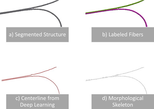
A natural approach to obtaining the discrete centerlines is skeletonization. Here, a binarized voxel image is selectively eroded until only a discretized curve with a thickness of a single voxel remains. However, because skeletonization is topology-preserving, it alone cannot entirely separate fibers that touch in the binarized image (see Figure 1). Unfortunately, this occurs quite frequently, either as an artifact of segmentation or because the fibers are physically connected, as in the case of thermally bonded materials. To avoid this problem, we use a neural network-based method to find the centerlines of fibers. The neural network labels voxels through which the centerline of a fiber passes in the image, which results in an image similar to skeletonization but without cross-linking neighboring fibers at contact points.

Figure 1. Two fibers cut out from nonwoven sample C are shown in image (a). The fibers are parallel and touch each other over a long distance. The result of labeling the individual fibers with our method is shown in image (b). The two fibers are correctly separated. The extracted fiber centerlines using the neural network approach are visualized in image (c). In contrast, the centerlines, as created by skeletonization, are shown in image (d).

Training data generation

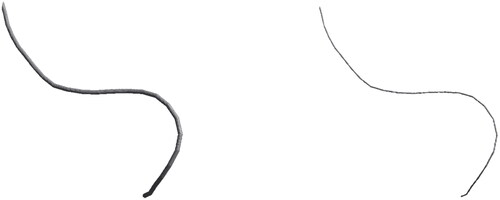
Labeling fiber centerlines manually would be very time-consuming. Therefore, to obtain the necessary training data, we use synthetic models generated from the ‘FiberGeo’ (Schladitz et al., 2006) fiber generation module, which is a component of the GeoDict (Becker et al., 2021) digital material laboratory. In these models, the analytic description of the fibers is available, and voxels containing the analytic centerline can be labeled easily (see Figure 2).

Figure 2. Generated fiber and the corresponding centerline obtained from the analytic model.

Sliding window

To avoid being limited to fixed image sizes, we do not apply the neural network to the whole image all at once. Instead, a sliding input window is passed over the image, and the neural network generates labels for a smaller output sub-window in the center. Because the neural network ‘sees’ only the contents of the input window, that window needs to be large enough to capture the fibers’ shape and local trajectory.

Neural network

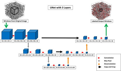
TensorFlow (Abadi et al., 2015) is used for the Deep Learning part of the algorithm. As a network architecture, we choose a variation of the widely used U-Net (Ronneberger et al., 2015) (see Figure 3). Presented initially to label 2 D microscopy images, we extend the network to a 3 D architecture like (Çiçek et al., 2016). The network, therefore, transforms a fixed-size 3 D input volume to a smaller 3 D output volume, which contains the predicted labels for the center region of the input. We train the neural network using supervised learning. This means that inputs and corresponding outputs are passed to the training algorithm. The network learns how to transform the input into the corresponding output using a gradient descent optimization. Using a 3 D network architecture instead of a 2 D slice-based approach comes at the cost of longer training times and a demand for more training data. The latter is largely irrelevant in our approach as the amount of training data that can be generated is practically unlimited, and the time for data generation is negligible with respect to the training time. The benefit of using the 3 D U-Net lies in the achieved quality of the results. A smooth and flicker-free result is generated by considering a 3 D context bigger than the network’s output size. To keep the size of the input window and the training times manageable, we reduced the depth of the U-Net to two but designed our training framework so that window sizes and network depth can be adjusted freely, up to the GPU memory limit.

Figure 3. The adapted U-Net 3 D architecture applied in our approach.

Need for a digital twin and training data

For the model to be applicable to real material scans, the synthetic fiber structures used during training should resemble these real materials, at least locally. A wide range of varying fiber structures can be generated quickly by sweeping through the parameters of the fiber generation module FiberGeo (Hilden et al., 2021). This approach allows us to obtain plenty of training data in a timely manner and avoids one of the main limitations of supervised learning approaches, the scarcity of training data. We generated curved fibers several times longer than the domain under consideration for the examples shared later in the results. The curvature was modeled so that both straight and curved segments were obtained. The fibers were mainly oriented in a plane, but a small amount of perpendicular deviation was permitted. Apart from the fiber trajectories, the contact points where fibers touch each other require particular attention. We applied morphological closing to match these contact areas’ appearance to the real micro-CT-scans. As the regions without fiber contacts proved easy for the network to label, we used training structures with an artificially high number of contact points such that these more complex configurations occur more frequently. This was done by simply increasing the density of fibers beyond the density found in the real materials, which naturally leads to more fiber contacts. To train the network, we generated nine artificial fiber structures with 512 by 512 by 256 voxels each (Figure 4).

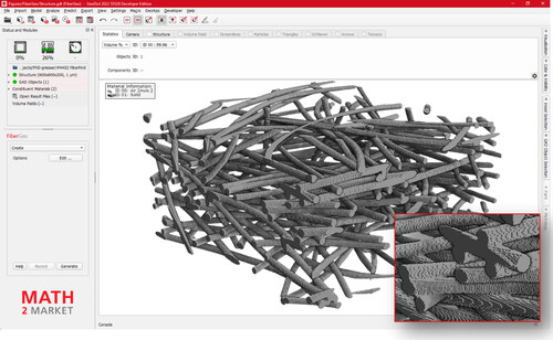
Figure 4. Example of fibrous training structure generated with FiberGeo (Hilden et al., 2021), including overlap by maximally 2 voxels and added artificial micro-CT scan artefact (highlighted in the small image).

Centerline to graph representation

Applying the network to a segmented scan results in labeled centerlines about three voxels in diameter. We further reduce the diameter to a single voxel by applying a skeletonization algorithm. These chains of adjacent voxels are then converted into a graph representation by starting at the end of a chain and tracing along the neighboring labeled voxels. Ideally, this yields a completely disconnected graph where every fiber is represented as two graph nodes connected by a single edge. The nodes correspond to the endpoints of the fiber, while the edge corresponds to the fiber trajectory. However, this might not be the case due to artifacts in the CT-scan or detection errors in the neural network. Some fibers might fall apart into multiple graph components, and therefore, we use a reconnection step to merge fiber fragments back together. The opposite case of fibers merging is a significant problem in skeletonization-only approaches. However, in our method, this artifact does not occur because fibers in the training data are guaranteed not to overlap so much that the centerlines touch; hence, the output inherits this property for real micro-CT scans.

Fragment reconnection

To reconnect the fiber fragments, we consider all pairs of fragment endpoints which are closer than a specific distance. We define Euclidean length $l_{ik}$ as the distance between two fiber endpoints and $d_i,$ ${ d}_k,$ and ${ d}_{ki},$ as the directions of the fiber segments and the directions of the segment between the endpoints. For each endpoint combination, an optimization criterion $o_{ik}$ is calculated. Different optimization criteria are used for straight or curved fibers, and Eq. (1)(1) $$o_{ik}=\frac{l_{ik}}{l_{\max }}\mathrm{*}{d}_i\mathrm{*}{\mathrm{ }d}_k\mathrm{ }+(1-\frac{l_{ik}}{l_{\max }})\text{ * }(d_i\mathrm{*}{\mathrm{ }d}_{ik}+d_k\mathrm{*}{\mathrm{ }d}_{ki})$$(1) is used for primarily straight fibers, and Eq. (2)(2) $$o_{ik}=d_i\mathrm{*}{\mathrm{ }d}_k+d_i\mathrm{*}{\mathrm{ }d}_{ik}+d_k\mathrm{*}{\mathrm{ }d}_{ki}\mathrm{ }$$(2) is used for curved Fibers. (1) $$o_{ik}=\frac{l_{ik}}{l_{\max }}\mathrm{*}{d}_i\mathrm{*}{\mathrm{ }d}_k\mathrm{ }+(1-\frac{l_{ik}}{l_{\max }})\text{ * }(d_i\mathrm{*}{\mathrm{ }d}_{ik}+d_k\mathrm{*}{\mathrm{ }d}_{ki})$$(1) (2) $$o_{ik}=d_i\mathrm{*}{\mathrm{ }d}_k+d_i\mathrm{*}{\mathrm{ }d}_{ik}+d_k\mathrm{*}{\mathrm{ }d}_{ki}\mathrm{ }$$(2)

The pair of fragments with the highest value for $o_{ik}$ are then connected (replaced by a single fragment) through interpolation to form a single fragment. We continue with the next best pair in a greedy strategy until no pair of endpoints with $o_{ik}$ larger than a given threshold remains. At the end of this procedure, all fibers in the scan are represented by a list of voxel coordinates connecting the start and end points.

Graph to analytical fiber

This list of voxel coordinates is converted into a piecewise linear fiber centerline by merging connections between two voxels so that the resulting line never deviates further than two voxels. This ensures that the noisy nature of the voxelized centerline is smoothed out, but the resulting centerline stays close to the actual position of the fiber. Then, the local diameter at each centerline point is determined by sampling the Euclidean distance map of the segmented CT-scan. In addition to obtaining the analytic fiber representations, we uniquely assign each fiber voxel in the original segmented scan to a fiber. For this purpose, we construct an object-label image where each voxel of a fiber’s centerline is assigned a unique ID corresponding to the fiber. Then a watershed (Beucher & Lantuéjoul, 1979) algorithm is used to completely label the fiber voxels surrounding the centerline with that same ID. After this procedure, every solid voxel has the unique ID of the fiber that it belongs to. Finally, we calculate the length, orientation, curvature, and curl-index (Corte & Kallmes, 1960; Page et al., 1985) of each fiber based on its analytic representation.

Fiber curvature and curl-index

The curvature of a fiber at a certain point is defined as the inverse of the radius of the tangential circle to the centerline. The fiber curl-index is the ratio between the curve length of the fiber and the Euclidean distance between the two fiber endpoints.

Advanced fiber analysis

In order to analyze the sample for gradients or inhomogeneities with respect to any of the computed properties, we can restrict the analysis to a sub-region of the sample domain. Additionally, it is possible to select a subset of fibers that fulfill a certain criterion and analyze only that subset for other properties (e. g., only analyze fibers above a particular length for curl-index as short fibers that intersect the domain boundary would skew the result). All algorithm steps are implemented with the option to use periodic boundary conditions to analyze unit cells of regular meshes (e.g. woven fabrics).

Validation

To validate that our approach can identify individual fibers, we created three additional synthetic structures for which the ground truth is known (Figure 5). The samples were created using FiberGeo with the parameters listed in Table 1.

Figure 5. Top: Validation sample 1 to 3. Bottom: Only the wrongly classified fibers, showing 13, 33 and 17 errors respectively from left to right.

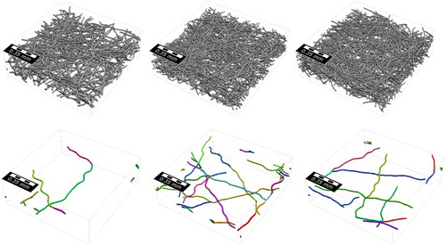
Table 1. Overview of the most important parameters used to generate the validation samples.

	Validation 1	Validation 2	Validation 3
Number of Fibers	221	407	339
Solid Volume Percentage/ (%)	9.4	10.8	11.9
Fiber Diameter/(µm)	16–19	13–16	13–16
Noise Artifacts	Yes	No	Yes

The fibers were allowed to overlap by 2 µm. The voxel length of the generated model is 2 µm. A small amount of binder was added to smooth out the contact points of fibers, making the model look closer to a micro-CT-scan. On top of this, in Validation Samples 1 and 3, stochastic noise was added to the surface of the fibers to simulate noise in the micro-CT-scan (Figure 6). In contrast to the training data, the fibers were generated slightly elliptical to simulate deformations that might happen during the manufacturing process and test how well the model generalizes to these cases. The results (see Figures 7 and 8) were inspected (see Figure 9), and the following four types of errors were observed:

Figure 6. Generated validation structure 3 with a solid volume percentage of 11.9% and 339 individual fibers.

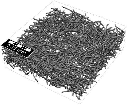
Figure 7. Left: ground truth of the validation structure 3 (every voxel is assigned to a fiber). Right: Result of the fiber identification algorithm.

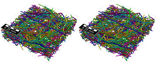
Figure 8. 2 D view of validation sample 3 and the fiber identification result. Even the artificially generated noise surfaces are labeled correctly.

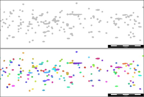
Figure 9. All fiber segments with errors in the result of the fiber identification process of validation sample 3. Most errors occur close to the boundary due to boundary error done by the neural network.

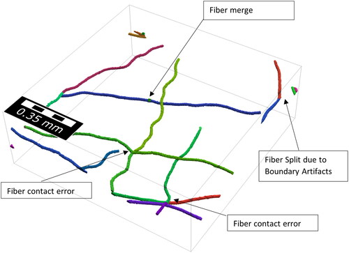
1. Boundary Artifacts: Due to the neural network always considering a localized window of 44x44x44 voxels errors in the centerline detection can occur near the boundary.

2. Fiber split: In some cases, fragmented fibers are not reconnected by the reconnection algorithm and a fiber may fall apart.

3. Fiber contact error: When fiber centerlines fall apart at a contact point, the fiber reconnection algorithm sometimes connects the wrong fiber ends because they exhibit similar distances and orientations as the correct pairing.

4. Fiber merge: When the endpoints of 2 fibers are close, the algorithm can wrongly merge them into one fiber in some cases.

We evaluated the occurrences of these errors for each of the 3 validation samples (Table 2).

Table 2. Error analysis of the validation samples showing the absolute and relative number of errors and error types for each validation sample

	Validation 1		Validation 2		Validation 3
	221		407		339
Number of fibers	Absolute	Relative	Absolute	Relative	Absolute	Relative
Boundary artifacts	11	5%	20	4.9%	12	3.5%
Fiber contact errors	0	0%	9	2.2%	5	1.5%
Fiber merges	2	1%	4	1%	0	0%
Total errors	13	5.9%	33	8.1%	17	5%

For all validation samples, the dominating error class is boundary errors. This is expected as the neural network is run with symmetric boundary conditions at the border of the structure. Fiber contact errors in validation sample 2 were mainly caused by 2 clusters of multiple thin fibers touching in the same place. We did not observe this configuration when validating on real images, however. The validation dataset and the results are available under https://doi.org/10.30423/data.math2market-2022-02.validation.fiberfind.

Results

We demonstrate our method on two material samples. The materials under consideration are bulky nonwoven fabrics. According to WO2020/103964 A1 (Kroutilova et al., 2020), these materials can be used in the hygiene industry as components of absorbent hygiene products (e. g. baby diapers, incontinence products, female hygiene products, changing pads, etc.).

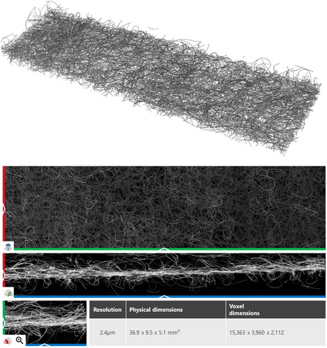
The two samples are composed of synthetic round fibers. The fiber diameter varies slightly within each sample, and the samples differ in fiber density and distribution of fibers. Bruker acquired multiple scans per sample on a SkyScan 1272 micro-CT. These individual scans were stitched together along the x-Axis to create the full-sized scan. The first sample, Sample C (Figure 10), was scanned at a resolution of 2.4 µm and has dimensions of 15,363 × 3,640 × 2,112 for a total of 118,958,443,614 voxels. Sample C is available for general access under https://doi.org/10.30423/data.math2market-2022-02.sample-c.fiberfind (Grießer et al., 2022). The dataset contains the original micro-CT, the segmented binary raw image, the labeled raw image where every fiber has its label, and the analytic description of the centerlines of the fibers.

Figure 10. 3 D and 2 D view of Sample C – this sample is provided online as scan and identified fibers under https://doi.org/10.30423/FiberFind.Nonwoven.SampleC-2022-01.

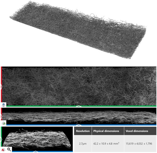
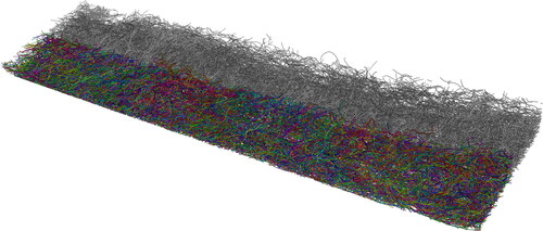
The second sample, Sample B (Figure 11), was scanned at a resolution of 2.7 µm and has dimensions of 15,619 × 4,032 × 1,796 for a total of 113,104,551,168 voxels.

Figure 11. 3 D and 2 D view of Sample B.

The sizes of the datasets required the algorithm to be extremely fast and memory efficient. Before taking the scans, the samples were aligned to have the principal fiber direction in the x-Axis so that the scans contain very long fiber segments.

We applied our method to both samples to characterize differences in the fiber geometry of the samples. The results of our analysis were used in the patent WO2020/103964 A1 (Kroutilova et al., 2020) to demonstrate differences between two manufacturing processes. The clear advantage of using the neural network-based centerline detection compared to morphological skeletonization can be seen in Figure 1 where the centerlines were calculated for two fibers that are in contact over a longer distance. The reconnection step can easily connect the gaps in the AI-derived centerline. In contrast, the morphological skeleton collapses to a single centerline in the area where the fibers are parallel. In Figure 12, a 2000 × 1000 × 2112 voxel sub-volume of Sample C can be seen where the fibers have been labeled with unique IDs. The IDs are visualized in distinct colors showing the successful identification of individual fibers in the complex fiber network. In Figure 13 the complete labeled fiber network of Sample C can be seen. Half of the domain shows the labeled voxels (colored), the other half shows the segmented structure (gray). Figure 14 shows the same result for the denser fiber network of Sample B. The training was done only once, and Sample B was analyzed using the neural network trained for Sample C. The models used in the training data were generic enough that the change in resolution between Sample C and Sample B did not negatively affect the results.

Figure 12. Sub-volume of Sample C (2000 by 1000 by 2112 Voxels) with labeled fibers.

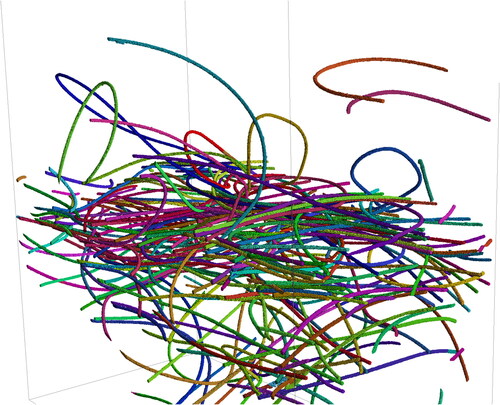
Figure 13. Split view of the Segmented Sample C and the labeled fibers colored in different colors.

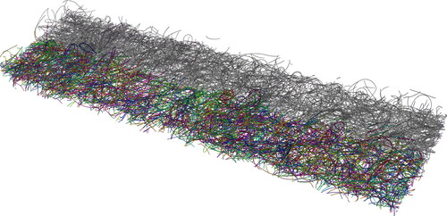
Figure 14. Split view of the Segmented Sample B and the labeled fibers colored in their individual colors.

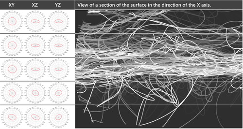
For Sample C the total number of fibers detected was 3352. For Sample B, 11,327 fibers were detected. Two geometric properties of the fibers of interest in the patent WO2020/103964 A1 (Kroutilova et al., 2020) are the distribution of fiber curvature and the distribution of the fiber curl-index. Particularly the analysis of the fiber curl-index made it necessary to use a large field of view for the scan. As visible in Figure 15, the trajectory of a single fiber within a nonwoven material can become complex and using only a small field of view would not reveal this. For the analyzed samples, the mean fiber curl-index of Sample C proved to be higher than the curl-index of sample B. For sample C the mean curl-index is 5.8; for sample B the mean curl-index is 2.9. This observation aligns well with the expectation of the manufacturer and the visual observation that Sample B generally looks more oriented in the machine direction (the x-Axis). The mean curvature of Sample B was measured to be lower too, matching the curl-index results (Figure 16). For Sample C the orientation was analyzed in multiple layers (Figure 17), revealing a stronger orientation in the machine direction towards the center of the material. In contrast, the top and bottom layers contain many fibers deviating in the Z-direction and later looping back into the main material sheet.

Figure 15. Some fibers of Sample B colored. The remaining fibers are rendered transparent.

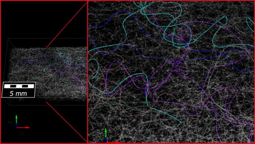
Figure 16. Comparison of the curvature distribution of sample B and C.

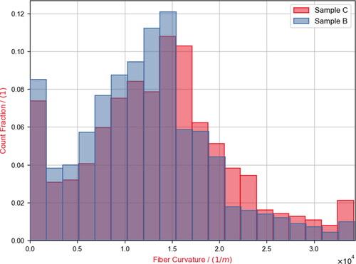
Figure 17. Orientation analysis of Sample C. The columns on the left show the orientation tensor visualized in the three main planes.

Conclusion

We demonstrate that our approach can identify individual fibers in CT-scans of nonwovens. The validation shows that the method is robust for samples that do not deviate too far from the parameters of the training data. We conclude that it is feasible to train neural networks on artificially generated models of nonwovens and apply them to the analysis of CT-scans of real materials. This method avoids the time-consuming and error-prone process of manually labeling data. It can be easily adapted to other fibrous materials by modifying the generator parameters. One such example could be fiber-reinforced composite materials.

Acknowledgements

We thank Michael Mass and Reicofil Reifenhäuser GmbH & Co. KG for letting us use, scan and analyze their materials and allowing us to provide sample C with this article. We thank Wesley De Boever and Bruker Corporation for scanning and stitching the micro-CT images.

Disclosure statement

The authors declare that they have no known competing interests that could have appeared to influence the work reported in this paper.

Correction Statement

This article has been corrected with minor changes. These changes do not impact the academic content of the article.

References

- Abadi, M., Agarwal, A., Barham, P., Brevdo, E., Chen, Z., Citro, C., … Zheng, X. (2015). TensorFlow: Large-scale machine learning on heterogeneous systems. Retrieved from https://arxiv.org/abs/1603.04467
- Axelsson, M. (2009). Estimating 3D fibre orientation in volume images < SE-END> [Paper presentation].</SE-END> January, 2008, pp. 1–4. https://doi.org/10.1109/ICPR.2008.4761631
- Badran, A., Marshall, D., Legault, Z., Makovetsky, R., Provencher, B., Piché, N., & Marsh, M. (2020). Automated segmentation of computed tomography images of fiber-reinforced composites by deep learning. Journal of Materials Science, 55(34), 16273–16289. https://doi.org/10.1007/s10853-020-05148-7
- Becker, J., Biebl, F., Cheng, L., Glatt, E., Grießer, A., Groß, M., … Wiegmann, A. (2021). September). GeoDict Software. GeoDict Software. Retrieved from https://www.math2market.de/GeoDict/geodict_download.php
- Beckman, I. P., Berry, G., Cho, H., & Riveros, G. (2021). Digital twin geometry for fibrous air filtration media. Fibers, 9(12), 84. https://doi.org/10.3390/fib9120084
- Beucher, S., & Lantuéjoul, C. (1979, January). Use of Watersheds in Contour Detection. 132.
- Çiçek, Ö., Abdulkadir, A., Lienkamp, S. S., Brox, T., & Ronneberger, O. (2016). 3D U-Net: Learning dense volumetric segmentation from sparse annotation. 3D U-Net: Learning dense volumetric segmentation from sparse annotation.
- Corte, H., & Kallmes, O. J. (1960). The structure of paper. I The statistical geometry ofindeal two dininsional fiber networks. Tappi Journal, 43(9), 737–752.
- Depriester, D., Rolland Du Roscoat, S., Orgéas, L., Geindreau, C., Levrard, B., & Brémond, F. (2022). Individual fibre separation in 3D fibrous materials imaged by X-ray tomography. Journal of Microscopy, 286(3), 220–239. https://doi.org/10.1111/jmi.13096
- Grießer, A., Westerteiger, R., Glatt, E., De Boever, W., Hagen, H., & Wiegmann, A. (2022). Identified fibers and validation data for fiber identification, https://doi.org/10.30423/data.math2market-2022-02.sample-c.fiberfind
- Henyš, P., & Čapek, L. (2021). Individual yarn fibre extraction from micro-CT: Multilevel machine learning approach. The Journal of The Textile Institute, 0, 1–8. https://doi.org/10.1080/00405000.2020.1865503
- Hilden, J., Rief, S., & Planas, B. (2021, August). FiberGeo User Guide 2022. Tech report. https://doi.org/10.30423/userguide.geodict2022-fibergeo
- Hoess, K. M., Hahn, F. J., Schmauder, S., & Keller, F. (2021). Predicting the mechanical behavior of a polypropylene-based nonwoven using 3D microstructural simulation. The Journal of The Textile Institute, 0, 1–12. https://doi.org/10.1080/00405000.2021.2001891
- Huang, X., Wen, D., Zhao, Y., Wang, Q., Zhou, W., & Deng, D. (2016). Skeleton-based tracing of curved fibers from 3D X-ray microtomographic imaging. Results in Physics, 6, 170–177. https://doi.org/10.1016/j.rinp.2016.03.008
- Kallel, H., & Joulain, K. (2022). Design and thermal conductivity of 3D artificial cross-linked random fiber networks. Materials & Design, 220, 110800. https://doi.org/10.1016/j.matdes.2022.110800
- Kermani, I. D., Schmitter, M., Eichinger, J. F., Aydin, R. C., & Cyron, C. J. (2021). Computational study of the geometric properties governing the linear mechanical behavior of fiber networks. Computational Materials Science, 199, 110711. https://doi.org/10.1016/j.commatsci.2021.110711
- Konopczyński, T., Kröger, T., Zheng, L., & Hesser, J. (2019). Instance segmentation of fibers from low resolution CT Scans via 3D deep embedding learning.
- Krause, M., Hausherr, J., Burgeth, B., Herrmann, C., & Krenkel, W. (2010). Determination of the fibre orientation in composites using the structure tensor and local X-ray transform. Journal of Materials Science, 45(4), 888–896. https://doi.org/10.1007/s10853-009-4016-4
- Kroutilova, J., Maas, M., Mecl, Z., Wagner, T., Klaska, F., & Kasparkova, P. (2020, May 28). Patent No. WO 2020/103964 A1. Retrieved from https://patents.google.com/patent/WO2020103964A1/en
- May, D., Willenbacher, B., Semar, J., Sharp, K., & Mitschang, P. (2020). Out-of-plane permeability of 3D woven fabrics for composite structures. The Journal of The Textile Institute, 111(7), 1047–1053. https://doi.org/10.1080/00405000.2019.1682759
- Page, D. H., Seth, R. S., Jorda, B. D., & Barb, M. C. (1985). Curl, crimps, kinks and microcompressions in pulp fibres - their origin, measurement and significance. In V. Punton (Ed.), Papermaking raw materials, Trans. VIIIth Fund. Res. Symp. Oxford (pp. 183–227).
- Pourdeyhimi, B., & Ramanathan, R. (1995). Image analysis method for estimating 2-D fiber orientation and fiber length in discontinuous fiber reinforced composites. Polymers and Polymer Composites, 3, 277–287.
- Rigby, A. J., Anand, S. C., & Horrocks, A. R. (1997). Textile materials for medical and healthcare applications. Journal of the Textile Institute, 88(3), 83–93. https://doi.org/10.1080/00405009708658589
- Ronneberger, O., Fischer, P., & Brox, T. (2015). U-Net: Convolutional networks for biomedical image segmentation. Medical Image Computing and Computer-Assisted Intervention (MICCAI). 9351, 234–241. Retrieved from http://lmb.informatik.uni-freiburg.de/Publications/2015/RFB15a
- Schladitz, K., Peters, S., Reinel-Bitzer, D., Wiegmann, A., & Ohser, J. (2006). Design of acoustic trim based on geometric modeling and flow simulation for nonwoven. Computational Materials Science, 38(1), 56–66. https://doi.org/10.1016/j.commatsci.2006.01.018
- Soltani, P., Johari, M., & Zarrebini, M. (2015, January). 3D fiber orientation characterization of nonwoven fabrics using X-ray Micro-computed Tomography. World Journal of Textile Engineering and Technology, 1, 41–47.
- Suragani Venu, L., Shim, E., Anantharamaiah, N., & Pourdeyhimi, B. (2012). Three-dimensional structural characterization of nonwoven fabrics. Microscopy and Microanalysis, 18(6), 1368–1379. https://doi.org/10.1017/S143192761201375X
- Townsend, P., Larsson, E., Karlson, T., Hall, S. A., Lundman, M., Bergström, P., Hanson, C., Lorén, N., Gebäck, T., Särkkä, A., & Röding, M. (2021). Stochastic modelling of 3D fiber structures imaged with X-ray microtomography. Computational Materials Science, 194, 110433. https://doi.org/10.1016/j.commatsci.2021.110433
- Viguié, J., Latil, P., Orgéas, L., Dumont, P. J. J., Rolland Du Roscoat, S., Bloch, J.-F., Marulier, C., & Guiraud, O. (2013). Finding fibres and their contacts within 3D images of disordered fibrous media. Composites Science and Technology, 89, 202–210. https://doi.org/10.1016/j.compscitech.2013.09.023
- Weber, M., Grießer, A., Glatt, E., Wiegmann, A., & Schmidt, V. (2022). Modeling curved fibers by fitting R-vine copulas to their Frenet representations. Accepted in Microscopy and Microanalysis.
- Westenberger, P., Estrade, P., & Lichau, D. (2012). Fibre orientation visualization with AvizoFire. NDTnet, Retrieved from https://www.ndt.net/search/docs.php3?id=13711#