Optimal control of motorsport differentials

Abstract

Modern motorsport limited slip differentials (LSD) have evolved to become highly adjustable, allowing the torque bias that they generate to be tuned in the corner entry, apex and corner exit phases of typical on-track manoeuvres. The task of finding the optimal torque bias profile under such varied vehicle conditions is complex. This paper presents a nonlinear optimal control method which is used to find the minimum time optimal torque bias profile through a lane change manoeuvre. The results are compared to traditional open and fully locked differential strategies, in addition to considering related vehicle stability and agility metrics. An investigation into how the optimal torque bias profile changes with reduced track-tyre friction is also included in the analysis. The optimal LSD profile was shown to give a performance gain over its locked differential counterpart in key areas of the manoeuvre where a quick direction change is required. The methodology proposed can be used to find both optimal passive LSD characteristics and as the basis of a semi-active LSD control algorithm.

Keywords:

• race car
• limited slip differential
• optimal control
• minimum time

1. Introduction

In the motorsport environment, where traction at one wheel is often compromised due to high cornering accelerations, Limited slip differentials (LSD) have been shown to offer significant improvements in traction and vehicle stability [1–3]. Fundamentally, LSDs are devices in which torque must be transferred from the faster to the slower rotating driven wheel. The direction of this torque transfer is determined by the driven wheel speed difference, which is strongly coupled to the longitudinal traction at each wheel. How the magnitude of this torque bias is controlled under certain conditions has evolved into two main strategies: semi-active and passive devices.

Although semi-active LSDs were prevalent in the World Rally Championship,[4] modern regulations now preclude the use of such devices in the majority of racing formula, with the exception of Formula 1 [5]. Even here, there are severe restrictions on the way in which control strategies are implemented. Only a limited number of vehicle parameters including longitudinal and lateral acceleration, speed and engine rpm can be used as the inputs to a lookup table style control strategy. The majority of other racing categories have relied on the use of passive devices, in which the torque bias magnitude is proportional to the differential input torque (torque sensing) or the driven wheel speed difference (speed sensing). Both semi-active and passive devices allow the level of torque bias to be controlled in various cornering phases, from the corner entry and apex, to the corner exit. These are effected either by steering wheel control dials (in the semi-active case), or through replacement of a number of key components in the LSD [1] (in the passive case).

With so many potential LSD setup parameters at an engineer's disposal, the task of optimising semi-active and passive characteristics to give the minimum manoeuvre time becomes complex. The motivation behind this paper therefore, is to present a method in which the optimal torque bias profile for a given manoeuvre can be found. This can then be used to either formulate improved semi-active control strategies, or fit against torque or speed sensing characteristics for improved passive setup configurations.

In [1,2], this task was addressed using a Quasi-Steady State (QSS) nonlinear constrained optimisation routine. The torque bias is included in the optimisation scheme, which is tasked with maximising the longitudinal and lateral acceleration limits of the vehicle in the form of a ‘GG’ type diagram. The inherent assumption with these methods is that the racing line is known, and the system transients can be neglected by assuming QSS cornering conditions.

Several researchers have developed more sophisticated dynamic time-optimal methods [3,6–9] which can generate the optimal control histories (throttle/brake and steering angle) and racing line for a given set of track boundaries. Crucially, these methods also allow the vehicle system dynamics to be included. As will be shown in this paper, this is a key consideration, since the influence of the transient vehicle yaw response to a steer input, what drivers refer to as ‘turn-in’ cannot be quantified (in terms of lap time) using traditional QSS methods. This is particularly relevant to the LSD application, since a common complaint amongst drivers is that over-aggressive strategies, (ones which promote high levels of torque bias) are detrimental to vehicle agility during the corner entry phase.

In the context of this work, the methods reported in [3,6] are most relevant, which employed nonlinear optimal control techniques to conduct a number of parametric studies with varying LSD torque bias parameters. Both studies considered a contemporary Formula 1 vehicle, with varying levels of torque bias from open (zero torque bias) to fully locked (in theory able to support an infinite torque bias). Kelly [3] considered fully open and locked differentials, in addition to two static torque sensing control strategies. The quickest configuration over a ${90}^{\circ }$ bend was found to be in-between the two extremes of LSD state. In [6], the LSD is one of four vehicle parameters which are optimised around a racing lap of the Barcelona circuit. The speed sensing LSD model used a differential viscosity factor to generate its torque bias and demonstrated that a locked differential yielded the minimum lap time. It should be noted that in both works, a pre-determined, or static configuration was maintained throughout the manoeuvre distance.

This paper investigates further performance potential available in allowing the torque bias strategy to vary along the manoeuvre length. The method presented ultimately allows more efficient parameter optimisation and greater insight into the optimal torque biasing control strategy.

The paper is organised into two main sections. In Section 2, a seven degree of freedom (DOF) planar vehicle model of a contemporary rear wheel drive (RWD) saloon racing vehicle is presented, along with a simplified Pacejka [10] tyre model of a representative racing slick tyre. An indirect nonlinear optimal control method [11] for a continuous system is then described. This includes a discussion of how the physical limitations of the driver and vehicle have been included in the process. In Section 3, this methodology is used to generate the associated steering, throttle and torque bias control histories that yield the minimum manoeuvre time solution over a typical lane change manoeuvre. Both the control histories and racing line are compared to open and fully locked differential solutions to investigate whether variations in differential configuration influences the optimal racing line. A discussion of the associated vehicle stability and agility is also included through the use of yaw stiffness and control derivatives [12].

Practical experience has shown that the levels of tyre wear and road friction also play an important role in the choice of optimal LSD strategy. This is addressed in the final part of this paper, where the lane change manoeuvre is repeated for varying levels of road friction, intended to represent intermediate and fully wet conditions. A qualitative analysis of tyre wear implications is included through consideration of the longitudinal frictional slip energy developed at each of the driven wheels.

2. Mathematical formulation

The following section details a seven DOF vehicle model, in addition to a nonlinear optimal control method used to generate minimum time solutions. Particular focus is given to the physical constraints of both the vehicle and driver, so that limits imposed on the torque bias, steering and throttle rates give an additional level of realism.

2.1. Vehicle model

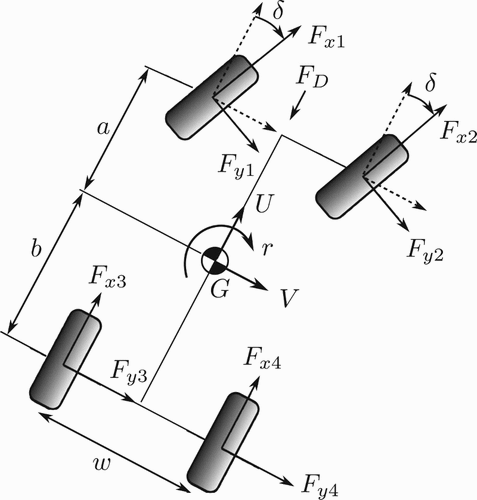
The vehicle model described in Figure 1 is based on the seven DOF planar model used in [1], which includes longitudinal, lateral and yaw rate motions in addition to four wheel rotations. This vehicle model was validated against experimental data produced from a qualifying lap of a RWD saloon racing vehicle. The simulated speed and acceleration histories were in close agreement, providing further confidence in the foundations of the work presented in this paper. The longitudinal (U), lateral (V ) and yaw (r) motions are defined by the equations: (1) $M(\dot{U}-Vr)=\cos \delta (F_{x1}+F_{x2})-\sin \delta (F_{y1}+F_{y2})+F_{x3}+F_{x4}-F_D$(1) (2) $M(\dot{V}+Ur)=\sin \delta (F_{x1}+F_{x2})+\cos \delta (F_{y1}+F_{y2})+F_{y3}+F_{y4}$(2) (3) $\begin{array}{rl}{J}_z\dot{r}& =(\cos \delta (F_{x1}-F_{x2})-\sin \delta (F_{y1}+F_{y2}\left)\right)\frac{w}{2}+(F_{x3}-F_{x4})\frac{w}{2}\\ & +a(\sin \delta (F_{x1}+F_{x2})+\cos \delta (F_{y1}+F_{y2}\left)\right)-b(F_{y3}+F_{y4})\end{array}$(3)

Figure 1. Vehicle model.

where M is the vehicle mass, $J_z$ is the yaw moment of inertia and δ the steered road wheel angle. w is the track width (equal at front and rear), a and b are the distances of the centre of mass (CoM) G from the front and rear axle, respectively, and $F_{x_i}$ and $F_{y_i}$ (where $i=\mathrm{1...4}$) the longitudinal and lateral tyre forces, respectively. $F_D$ represents a longitudinal drag force component. The front undriven ${\omega }_{1,2}$ and rear driven ${\omega }_{3,4}$ wheel motions are defined by: (4) $J_w{\dot{\omega }}_i=T_i-F_{x_i}R,i=1\dots 4,$(4) where $J_w$ is the rotational inertia, R the wheel radius, ${\omega }_i$ are the wheel speeds and $T_i$ the torque at each wheel (braking for $T_{1,2}$, propulsive or braking for $T_{3,4}$). The engine and brake torque characteristics are included through the use of torque control input ${\gamma }_t$. This represents the total driving/braking torque at any instant and splits engine and brake torque between the front and rear axles using the distribution factor $k_t$. The value of $k_t$ alternates between acceleration and braking events (see Table 1). The LSD torque bias $T_b$ is included at the rear wheels, with the direction of torque transfer constrained to travel from the faster to slower rotating wheel. Assuming power losses in the differential are neglected, the resultant torque at each wheel can therefore be described by : (5) $T_1=\frac{(1-k_t){\gamma }_t}{2}{T}_2=\frac{(1-k_t){\gamma }_t}{2},$(5) (6) $T_3=\frac{k_t{\gamma }_t}{2}+T_b{T}_4=\frac{k_t{\gamma }_t}{2}-T_b.$(6) It should be noted that the total difference between rear left and right wheel torque is $T_3-T_4=2T_b$. The direction of the torque bias is constrained to reflect the sign of the speed difference between driven wheels such that: (7) $\mathrm{sgn}\left(T_b\right)=\mathrm{sgn}({\omega }_3-{\omega }_4).$(7)

In the case of a locked differential, the rear wheel equations can be combined to give the rear axle speed ${\omega }_r$, where ${\omega }_r={\omega }_3={\omega }_4$. Equation (4(4) $J_w{\dot{\omega }}_i=T_i-F_{x_i}R,i=1\dots 4,$(4) ) can therefore be simplified for the case of $i=3,4$ to give: (8) $2J_w{\dot{\omega }}_r=T_3+T_4-(F_{x3}+F_{x4})R.$(8) The longitudinal and lateral tyre forces depend on lateral slip α, longitudinal slip κ and the normal load $F_z$ on each tyre: (9) $F_{x_i}=F_{x_i}({\alpha }_i,{\kappa }_i,F_{z_i}),$(9) (10) $F_{y_i}=F_{y_i}({\alpha }_i,{\kappa }_i,F_{z_i}),$(10) where the slip quantities are defined as: (11) ${\alpha }_1=\delta +\frac{-V-ar}{U+rw/2}{\kappa }_1=\frac{{\omega }_{1}R-(U+rw/2)}{U+rw/2}$(11) (12) ${\alpha }_2=\delta +\frac{-V-ar}{U-rw/2}{\kappa }_2=\frac{{\omega }_{2}R-(U-rw/2)}{U-rw/2}$(12) (13) ${\alpha }_3=\frac{-V+br}{U+rw/2}{\kappa }_3=\frac{{\omega }_{3}R-(U+rw/2)}{U+rw/2}$(13) (14) ${\alpha }_4=\frac{-V+br}{U-rw/2}{\kappa }_4=\frac{{\omega }_{4}R-(U-rw/2)}{U-rw/2},$(14) while the dynamic normal tyre loads $F_{zi}$ are computed from a steady state approximation $F_{z{s}_i}$, combined with a first order lag function to account for suspension dynamics: (15) ${\tau }_z{\dot{F}}_{z_i}+F_{z_i}=F_{z{s}_i}\mathrm{for}i=1\dots 4,$(15) where ${\tau }_z$ denotes the suspension lag time constant. The steady state normal loads are a combination of the static weight distribution, longitudinal $a_x$, lateral $a_y$ accelerations and aerodynamic load influences such that: (16) $F_{zs1}=\frac{1}{2}\frac{Mgb}{a+b}-\frac{1}{2}\frac{M{a}_{x}h}{a+b}+\frac{M{a}_{y}h\xi }{w}-\frac{1}{2}\frac{F_D{h}_a}{a+b}-\frac{1}{2}\frac{F_L{b}_a}{a+b}$(16) (17) $F_{zs2}=\frac{1}{2}\frac{Mgb}{a+b}-\frac{1}{2}\frac{M{a}_{x}h}{a+b}-\frac{M{a}_{y}h\xi }{w}-\frac{1}{2}\frac{F_D{h}_a}{a+b}-\frac{1}{2}\frac{F_L{b}_a}{a+b}$(17) (18) $F_{zs3}=\frac{1}{2}\frac{Mga}{a+b}+\frac{1}{2}\frac{M{a}_{x}h}{a+b}+\frac{M{a}_{y}h\left(1-\xi \right)}{w}+\frac{1}{2}\frac{F_D{h}_a}{a+b}-\frac{1}{2}\frac{F_L{a}_a}{a+b}$(18) (19) $F_{zs4}=\frac{1}{2}\frac{Mga}{a+b}+\frac{1}{2}\frac{M{a}_{x}h}{a+b}-\frac{M{a}_{y}h\left(1-\xi \right)}{w}+\frac{1}{2}\frac{F_D{h}_a}{a+b}-\frac{1}{2}\frac{F_L{a}_a}{a+b},$(19) where h is the height of the CoM G from the ground, ξ the front roll stiffness distribution factor, $h_a$ the height of the aerodynamic centre of pressure (CoP), and $a_a$, $b_a$ the distances of the CoP from the front and rear axles, respectively. Gyroscopic forces from wheel rotations have been neglected. The aerodynamic drag $F_D$ and lift $F_L$ forces are computed as follows: (20) $F_D=\frac{1}{2}\rho C_{D}A{U}^2$(20) (21) $F_L=\frac{1}{2}\rho C_{L}A{U}^2$(21) where ρ is the air density, $C_D$ and $C_L$ are the drag and lift coefficients and A is the frontal area. The position and orientation of the vehicle on the track is governed by the curvilinear coordinate system shown in Figure 2. Three additional coordinates are defined as the position of the vehicle along the track centreline $s_s$, its lateral position $s_n$ and the angle χ of the vehicle with respect to the tangent point on the track.

Figure 2. Curvilinear track coordinate system.

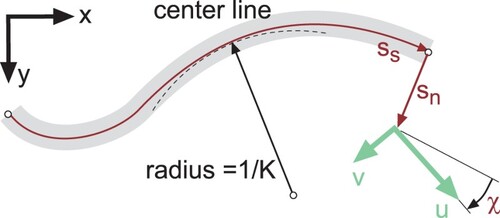
Table 1. Parameters of RWD vehicle model.

Parameter	Symbol	Value	Unit
Mass	M	1200	kg
Yaw inertia	$J_z$	1700	kg m${}^2$
Height of CoM	h	0.45	m
Distance of CoM from rear	b	1.4	m
Distance of CoM from front	a	1.3	m
Track width	w	1.6	m
Wheel inertia	$J_w$	1.8	kg m${}^2$
Wheel radius	R	0.3	m
Drag	$C_{D}A$	0.88	m${}^2$
Lift	$C_{L}A$	−0.1	m${}^2$
Air density	ρ	1.2	kg/m${}^3$
Roll stiffness ratio	ξ	0.53	–
Suspension time-lag	${\tau }_z$	0.2	s
Distance of CoP from rear	$b_a$	1.35	m
Distance of CoP from front	$a_a$	1.35	m
Braking torque distribution	$k_t$	0.48	–
Propulsive torque distribution	$k_t$	1.00	–

The differential equations relating the vehicle motions to the track coordinate system can be described by: (22) ${\dot{s}}_s=\frac{U\cos \chi -V\sin \chi }{1-s_{n}K}$(22) (23) $\dot{s_n}=U\sin \chi +V\cos \chi$(23) (24) $\dot{\chi }=r-K\frac{U\cos \chi -V\sin \chi }{1-s_{n}K},$(24) where K is the local curvature of the road. The resulting vehicle and track model can therefore be represented by a system of 14 nonlinear differential equations in Equations  (1(1) $M(\dot{U}-Vr)=\cos \delta (F_{x1}+F_{x2})-\sin \delta (F_{y1}+F_{y2})+F_{x3}+F_{x4}-F_D$(1) )–(4(4) $J_w{\dot{\omega }}_i=T_i-F_{x_i}R,i=1\dots 4,$(4) ), (15(15) ${\tau }_z{\dot{F}}_{z_i}+F_{z_i}=F_{z{s}_i}\mathrm{for}i=1\dots 4,$(15) ), (22(22) ${\dot{s}}_s=\frac{U\cos \chi -V\sin \chi }{1-s_{n}K}$(22) )–(24(24) $\dot{\chi }=r-K\frac{U\cos \chi -V\sin \chi }{1-s_{n}K},$(24) ). Thus, the state vector $\mathbf{\text{x}}$ can be described by: (25) $\mathbf{\text{x}}=\{U,V,r,{\omega }_1,{\omega }_2,{\omega }_3,{\omega }_4,F_{z1},F_{z2},F_{z3},F_{z4},s_s,s_n,\chi {\}}^{\mathrm{T}}.$(25) The control vector $\mathbf{\text{u}}$ consists of the steering, throttle/brake and torque bias inputs such that: (26) $\mathbf{\text{u}}=\{\delta ,{\gamma }_t,T_b{\}}^{\mathrm{T}}.$(26) The vehicle and track parameters of the RWD saloon racing vehicle considered in this paper are summarised in Table 1.

2.2. Tyre model

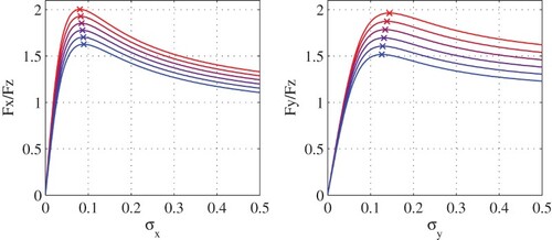
Tyre forces were calculated using a hybrid 1996 Pacejka Magic Formula model,[10] parameterised around tyre manufacturer test rig data for a 235/610R17 racing slick. The standard model requires over 50 parameters to describe the resultant longitudinal and lateral tyre forces as a function of slip angle ${\alpha }_i$, slip ratio ${\kappa }_i$, normal load $F_{zi}$ and camber angle. Due to the complexity of the optimal control method presented in Section 2.3, the model was simplified to increase robustness and reduce simulations run times. The aspects of the tyre model which dominate tyre force generation are retained with the use of only 13 parameters and are detailed in Table 2. In addition to the established coupling between longitudinal and lateral forces, three dominant behaviours were retained from the full Pacejka model. These were considered essential for representative results and are detailed as follows: (i) a decrease in the longitudinal and lateral friction coefficients with normal load, (ii) variation in the slip angle and slip ratio at which peak lateral and longitudinal forces are generated and (iii) nonlinear reduction in the longitudinal and lateral slip stiffness with normal load.

Table 2. Simplified Pacejka model coefficients.

Symbol	Description
$F_{z0}$	Reference normal load where $\mathrm{d}f=0$ (N)
$p{K}_{x1}$	Max longitudinal stiffness coefficient
$p{K}_{y1}$	Max cornering stiffness coefficient
$p{K}_{x3}$	Max longitudinal stiffness coefficient
$p{K}_{y2}$	Max cornering stiffness coefficient
$p{C}_{x1}$	Longitudinal shape factor
$p{C}_{y1}$	Lateral shape factor
$p{D}_{x1}$	Max longitudinal friction coefficient
$p{D}_{y1}$	Max lateral friction coefficient
$p{D}_{x2}$	Longitudinal friction load dependency factor
$p{D}_{y2}$	Lateral friction load dependency factor
$p{E}_{x1}$	Longitudinal curvature factor
$p{E}_{y1}$	Lateral curvature factor

The derivation presented below is taken from Ch. 4 of [10]. The theoretical longitudinal slip ${\sigma }_x$, lateral slip ${\sigma }_y$ and equivalent slip σ quantities can be evaluated from the practical slip values κ and α using: (27) ${\sigma }_x=\frac{\kappa }{1+\kappa }{\sigma }_y=\frac{\tan \alpha }{1+\kappa }\sigma =\sqrt{{{\sigma }_x}^2+{{\sigma }_y}^2}.$(27) The resulting longitudinal $F_x$ and lateral $F_y$ forces can then be found using the traditional Magic Formula expressions: (28) $F_x=\frac{{\sigma }_x}{\sigma }{D}_x\sin (C_x\arctan (B_x\sigma -E_x(B_x\sigma -\arctan (B_x\sigma \left)\right)\left)\right)F_z$(28) (29) $F_y=\frac{{\sigma }_y}{\sigma }{D}_y\sin (C_y\arctan (B_y\sigma -E_y(B_y\sigma -\arctan (B_y\sigma \left)\right)\left)\right)F_z.$(29) The parameters $B_{x,y}$, $C_{x,y}$, $D_{x,y}$, $E_{x,y}$ are defined at a particular reference tyre load $F_{z0}$, and the normalised change in vertical load is employed to linearly scale the peak friction coefficient $D_{x,y}$ parameter: (30) $\mathrm{d}{f}_z=\frac{F_z-F_{z0}}{F_{z0}}.$(30) For longitudinal tyres forces, the slip stiffness (slope at the origin) is defined by: (31) $K_x=F_{z}p{K}_{x1}\exp \left(p{K}_{x3}\mathrm{d}{f}_z\right),$(31) where the parameters $B_x$, $C_x$ and $D_x$ are: (32) $E_x=p{E}_{x1}$(32) (33) $D_x=(p{D}_{x1}+p{D}_{x2}\mathrm{d}{f}_z){\lambda }_{\mu ,x}$(33) (34) $C_x=p{C}_{x1}$(34) (35) $B_x=\frac{K_x}{C_x{D}_x{F}_z}$(35) The scaling factor ${\lambda }_{\mu ,x}$ was used to reduce the friction levels for the analysis presented in Section 6. Similarly for lateral tyre forces, the slip stiffness (slope at the origin) can be described by: (36) $K_y=p{K}_{y1}{F}_{z0}\sin \left(2\arctan \frac{F_z}{p{K}_{y2}{F}_{z0}}\right),$(36) where $B_y$, $C_y$ and $D_y$ are: (37) $E_y=p{E}_{y1}$(37) (38) $D_y=(p{D}_{y1}+p{D}_{y2}\mathrm{d}{f}_z){\lambda }_{\mu ,y}$(38) (39) $C_y=p{C}_{y1}{B}_y=\frac{K_y}{C_y{D}_y{F}_z}$(39) (40) $B_y=\frac{K_y}{C_y{D}_y{F}_z}$(40) ${\lambda }_{\mu ,y}$ is again the appropriate scaling factor in the lateral direction. The normalised longitudinal and lateral force curves are shown in Figure 3. The maximum friction coefficients reduce significantly as the load increases from 0.5 to 5.5 kN, in both longitudinal and lateral directions. The position of the peak longitudinal friction moves towards larger slip ratios as the normal load increases, while the peak lateral friction moves towards smaller slip angles. Crucially, for both longitudinal and lateral forces, the slip stiffness reduces as the normal load increases.

Figure 3. Normalised longitudinal (left) and lateral (right) tyre forces, for normal loads from 500N (red) to 5500N (blue) in steps of 1000N.

2.3. Optimal control method

An indirect nonlinear optimal control method is adopted which is based on the previous works [9,13,14]. This relies on the optimisation of the control vector elements until the performance index (in this case manoeuvre time) has been minimised, whilst a number of equality and inequality constraints are satisfied. An overview of the necessary conditions for optimality are given below, but the reader is referred to [11,14,15] for a more detailed treatise.

The variational formulation of the optimal control problem involves finding the control vector $\mathbf{\text{u}}\left(s\right)\in {\mathbb{R}}^m$ which minimises the cost functional: (41) $J\left[\mathbf{\text{x,u}}\right]={\int }_{s_i}^{s_f}f\left(\mathbf{\text{x}}\right(s),\mathbf{\text{u}}(s\left)\right)\mathrm{d}s,$(41) where $\mathbf{\text{x}}\left(s\right)\in {\mathbb{R}}^n$ represents the state vector, s the distance along the track in the curvilinear coordinate system and $s_i$, $s_f$ the distance interval. In this case, the cost functional is: (42) $J\left[\mathbf{\text{x,u}}\right]={\int }_{s_i}^{s_f}{S}_f\left(s\right)\mathrm{d}s,$(42) where $S_f\left(s\right)$ is (43) $S_f\left(s\right)={\left(\frac{\mathrm{d}s}{\mathrm{d}t}\right)}^{-1}=\frac{1-s_{n}K}{U\cos \chi -V\sin \chi }.$(43) The equations defined in Equations  (1(1) $M(\dot{U}-Vr)=\cos \delta (F_{x1}+F_{x2})-\sin \delta (F_{y1}+F_{y2})+F_{x3}+F_{x4}-F_D$(1) )–(4(4) $J_w{\dot{\omega }}_i=T_i-F_{x_i}R,i=1\dots 4,$(4) ), (15(15) ${\tau }_z{\dot{F}}_{z_i}+F_{z_i}=F_{z{s}_i}\mathrm{for}i=1\dots 4,$(15) ), (22(22) ${\dot{s}}_s=\frac{U\cos \chi -V\sin \chi }{1-s_{n}K}$(22) )–(24(24) $\dot{\chi }=r-K\frac{U\cos \chi -V\sin \chi }{1-s_{n}K},$(24) ) must be satisfied at all times. As a result, these ordinary differential equations can be represented as a constraint of the form: (44) $\mathbf{\text{A}}\left(\mathbf{\text{x}}\right)\dot{\mathbf{\text{x}}}+\mathbf{\text{b(x,u)}}=0,s\in (s_i,s_f).$(44) Additional constraints on the system are included through the use of equality and inequality constraints. An array of vector equality constraints $\mathbf{\text{c}}$ is used to set the initial and final boundary conditions as follows: (45) $\mathbf{\text{c}}\left(\mathbf{\text{x}}\right(s_i),\mathbf{\text{x}}(s_f\left)\right)=0.$(45) Table 3 summarises the initial and final boundary conditions of the 14 model variables defined in Equation (25(25) $\mathbf{\text{x}}=\{U,V,r,{\omega }_1,{\omega }_2,{\omega }_3,{\omega }_4,F_{z1},F_{z2},F_{z3},F_{z4},s_s,s_n,\chi {\}}^{\mathrm{T}}.$(25) ).The inequality constraints are set along the state trajectory with an array of vector quantities $\mathbf{\text{d}}$, such that:

Table 3. Initial and final boundary condition (BC) summary.

Variable	Symbol	Initial BC	Final BC	Unit
Longitudinal velocity	U	33	Free	m/s
Lateral velocity	V	0	Free	m/s
Yaw rate	r	0	0	rad/s
Wheel angular velocity	${\omega }_{\mathrm{1..4}}$	Free rolling	Free	rad/s
Tyre normal load	$F_{z\mathrm{1..}z4}$	Static value	Free	N
Distance along track centreline	$s_s$	0	Free	m
Lateral centreline offset	$s_n$	Free	Free	m
Heading angle	χ	Free	Free	rad

(46) $\mathbf{\text{d}}\left(\mathbf{\text{x}}\right(s),\mathbf{\text{x}}(s\left)\right)\le 0,s\in (s_i,s_f).$(46) The inequality constraints are included in the cost functional (Equation (41(41) $J\left[\mathbf{\text{x,u}}\right]={\int }_{s_i}^{s_f}f\left(\mathbf{\text{x}}\right(s),\mathbf{\text{u}}(s\left)\right)\mathrm{d}s,$(41) )) through the use of penalty functions,[16] which increase sharply if the inequality constraints are violated. The differential and equality constraints (Equations (44(44) $\mathbf{\text{A}}\left(\mathbf{\text{x}}\right)\dot{\mathbf{\text{x}}}+\mathbf{\text{b(x,u)}}=0,s\in (s_i,s_f).$(44) ) and (45(45) $\mathbf{\text{c}}\left(\mathbf{\text{x}}\right(s_i),\mathbf{\text{x}}(s_f\left)\right)=0.$(45) )) are included with the Lagrange multipliers $\mathit{\mu }$, $\mathit{\lambda }$. The augmented form of the cost functional $\tilde{J}$ can then be described as follows: (47) $\tilde{J}\left[\mathbf{\text{x,u,}}\mathit{\mu }\mathbf{,}\mathit{\lambda }\right]=\mathit{\mu }\cdot \mathbf{\text{c}}\left(\mathbf{\text{x}}\right(s_i),\mathbf{\text{x}}(s_f\left)\right)+{\int }_{s_0}^{s_f}\left[f_p\right(\mathbf{\text{x}}\left(s\right),\mathbf{\text{u}}\left(s\right))+\mathit{\lambda }(s)\cdot \mathbf{\text{A}}(x)\dot{x}+\mathbf{\text{b(x,u)}}]\mathrm{d}s,$(47) where (48) $f_p(\mathbf{\text{x}},\mathbf{\text{u}})=f(\mathbf{\text{x}},\mathbf{\text{u}})+\sum _{i=1}^q{p}_i\left(d_i\right(\mathbf{\text{x}},\mathbf{\text{u}}\left)\right),$(48) for a total of q inequality constraints, where $p_i$ is the penalty function associated with the ith component of Equation (46(46) $\mathbf{\text{d}}\left(\mathbf{\text{x}}\right(s),\mathbf{\text{x}}(s\left)\right)\le 0,s\in (s_i,s_f).$(46) ) and takes the form [17]: (49) $p_i(h_i,d_i,n)=\left\{\begin{array}{ll}0& d_i<0,\\ {\left(\frac{d_i}{h_i}\right)}^n& d_i\ge 0,i=1\dots q\end{array}\right.$(49) $h_i$ defines the length of the region for which the resulting penalty function value will be zero (or very close to it) and dictates the point at which the inequality constraint becomes active. n is used to control the sharpness of the function when the limiting value has been exceeded, and $d_i$, is the associated constrained parameter (see Equations (59(59) $|\delta |\le {\delta }_{max}.$(59) )–(65(64) $-t_l\le s_n-b\sin \chi \le t_r,$(64) ) in Section 2.3.1).

By taking partial derivatives of Equation (47(47) $\tilde{J}\left[\mathbf{\text{x,u,}}\mathit{\mu }\mathbf{,}\mathit{\lambda }\right]=\mathit{\mu }\cdot \mathbf{\text{c}}\left(\mathbf{\text{x}}\right(s_i),\mathbf{\text{x}}(s_f\left)\right)+{\int }_{s_0}^{s_f}\left[f_p\right(\mathbf{\text{x}}\left(s\right),\mathbf{\text{u}}\left(s\right))+\mathit{\lambda }(s)\cdot \mathbf{\text{A}}(x)\dot{x}+\mathbf{\text{b(x,u)}}]\mathrm{d}s,$(47) ) and setting it to zero, the following differential algebraic, boundary value expressions can be derived [14]: (50) $\frac{\mathrm{\partial }\tilde{d}(\mathbf{\text{x}},\mathbf{\text{u}},\mathit{\lambda })}{\mathrm{\partial }\mathbf{\text{x}}}+\mathbf{\text{T}}(\mathbf{\text{x}},\mathit{\lambda }{)}^{\mathrm{T}}\dot{\mathbf{\text{x}}}-{\mathbf{\text{A(x)}}}^{\mathrm{T}}\dot{\mathit{\lambda }}=0$(50) (51) $\mathbf{\text{A}}\left(\mathbf{\text{x}}\right)\dot{\mathbf{\text{x}}}+\mathbf{\text{b(x,u)}}=0$(51) (52) $\frac{\mathrm{\partial }\tilde{d}(\mathbf{\text{x}},\mathbf{\text{u}},\mathit{\lambda })}{\mathrm{\partial }\mathbf{\text{u}}}=0$(52) (53) $\frac{\mathrm{\partial }e\left(\mathbf{\text{x}}\right(s_i),\mathbf{\text{x}}(s_f),\mathit{\mu }{)}^{\mathrm{T}}}{\mathrm{\partial }\mathbf{\text{x}}\left(s_f\right)}+\mathit{\omega }\left(\mathbf{\text{x}}\right(s_f),\mathit{\lambda }(s_f\left)\right)=0$(53) (54) $\frac{\mathrm{\partial }e\left(\mathbf{\text{x}}\right(s_i),\mathbf{\text{x}}(s_f),\mathit{\mu }{)}^{\mathrm{T}}}{\mathrm{\partial }\mathbf{\text{x}}\left(s_i\right)}+\mathit{\omega }\left(\mathbf{\text{x}}\right(s_i),\mathit{\lambda }(s_i\left)\right)=0$(54) (55) $\mathbf{\text{c}}\left(\mathbf{\text{x}}\right(s_i),\mathbf{\text{x}}(s_f\left)\right)=0$(55) where (56) $\tilde{d}(\mathbf{\text{x}},\mathbf{\text{u}},\mathit{\lambda })=f_p(\mathbf{\text{x}},\mathbf{\text{u}})+{\mathit{\lambda }}^{\mathrm{T}}\mathbf{\text{b(x,u)}}$(56) (57) $\omega (\mathbf{\text{x}},\mathit{\lambda })={\mathbf{\text{A(x)}}}^{\mathrm{T}}\mathit{\lambda }.$(57) (58) $\mathbf{\text{T}}(\mathbf{\text{x}},\mathit{\lambda }{)}^{\mathrm{T}}=\frac{\mathrm{\partial }\omega (\mathbf{\text{x}},\mathit{\lambda })}{\mathrm{\partial }\mathbf{\text{x}}}-\frac{\mathrm{\partial }\omega (\mathbf{\text{x}},\mathit{\lambda }{)}^{\mathrm{T}}}{\mathrm{\partial }\mathbf{\text{x}}}.$(58) In practice, due to the complexity of deriving Equations (50(50) $\frac{\mathrm{\partial }\tilde{d}(\mathbf{\text{x}},\mathbf{\text{u}},\mathit{\lambda })}{\mathrm{\partial }\mathbf{\text{x}}}+\mathbf{\text{T}}(\mathbf{\text{x}},\mathit{\lambda }{)}^{\mathrm{T}}\dot{\mathbf{\text{x}}}-{\mathbf{\text{A(x)}}}^{\mathrm{T}}\dot{\mathit{\lambda }}=0$(50) )–(55(55) $\mathbf{\text{c}}\left(\mathbf{\text{x}}\right(s_i),\mathbf{\text{x}}(s_f\left)\right)=0$(55) ), this process is carried out symbolically with the use of a bespoke MAPLE library. The initial conditions are described by Equation (54(54) $\frac{\mathrm{\partial }e\left(\mathbf{\text{x}}\right(s_i),\mathbf{\text{x}}(s_f),\mathit{\mu }{)}^{\mathrm{T}}}{\mathrm{\partial }\mathbf{\text{x}}\left(s_i\right)}+\mathit{\omega }\left(\mathbf{\text{x}}\right(s_i),\mathit{\lambda }(s_i\left)\right)=0$(54) ), with the final boundary conditions in Equation (53(53) $\frac{\mathrm{\partial }e\left(\mathbf{\text{x}}\right(s_i),\mathbf{\text{x}}(s_f),\mathit{\mu }{)}^{\mathrm{T}}}{\mathrm{\partial }\mathbf{\text{x}}\left(s_f\right)}+\mathit{\omega }\left(\mathbf{\text{x}}\right(s_f),\mathit{\lambda }(s_f\left)\right)=0$(53) ). The set of differential expressions describing the vehicle and track model are defined by Equation (51(51) $\mathbf{\text{A}}\left(\mathbf{\text{x}}\right)\dot{\mathbf{\text{x}}}+\mathbf{\text{b(x,u)}}=0$(51) ), the co-state equations in Equation (50(50) $\frac{\mathrm{\partial }\tilde{d}(\mathbf{\text{x}},\mathbf{\text{u}},\mathit{\lambda })}{\mathrm{\partial }\mathbf{\text{x}}}+\mathbf{\text{T}}(\mathbf{\text{x}},\mathit{\lambda }{)}^{\mathrm{T}}\dot{\mathbf{\text{x}}}-{\mathbf{\text{A(x)}}}^{\mathrm{T}}\dot{\mathit{\lambda }}=0$(50) ) and the optimality equation in Equation (52(52) $\frac{\mathrm{\partial }\tilde{d}(\mathbf{\text{x}},\mathbf{\text{u}},\mathit{\lambda })}{\mathrm{\partial }\mathbf{\text{u}}}=0$(52) ).

The differential-algebraic system is then discretised to obtain a finite dimensional algebraic problem. The distance interval ($s_i,s_f$) is split into P subintervals, and the optimality equation is evaluated at the collocation node $s_{k+\frac{1}{2}}=(s_k+s_{k+1})/2$, the midpoint of the interval ($s_k,s_{k+1}$), where $k=\mathrm{1...}P$. For the lane change considered in subsequent sections, P was assigned a value of 1500 intervals, equispaced over the manoeuvre distance (giving a spacing of approximately 0.25m between grid points). The co-state (Equation (50(50) $\frac{\mathrm{\partial }\tilde{d}(\mathbf{\text{x}},\mathbf{\text{u}},\mathit{\lambda })}{\mathrm{\partial }\mathbf{\text{x}}}+\mathbf{\text{T}}(\mathbf{\text{x}},\mathit{\lambda }{)}^{\mathrm{T}}\dot{\mathbf{\text{x}}}-{\mathbf{\text{A(x)}}}^{\mathrm{T}}\dot{\mathit{\lambda }}=0$(50) )) and differential equations describing the vehicle model (Equation (51(51) $\mathbf{\text{A}}\left(\mathbf{\text{x}}\right)\dot{\mathbf{\text{x}}}+\mathbf{\text{b(x,u)}}=0$(51) )) are approximated using the midpoint quadrature rule to average on ($s_k,s_{k+1}$) and by using finite differences in place of derivatives terms. In this instance, the numerical solver described by Bertolazzi, Biral, and Da Lio [14] was used, since it includes a number of efficiencies to increase robustness and reduce solve times.

2.3.1. Inequality constraints

In order to replicate the physical limitations of the vehicle, track and driver, a number of inequality constraints are included in the problem definition. These are enforced through the inclusion of penalty functions (see Equation (49(49) $p_i(h_i,d_i,n)=\left\{\begin{array}{ll}0& d_i<0,\\ {\left(\frac{d_i}{h_i}\right)}^n& d_i\ge 0,i=1\dots q\end{array}\right.$(49) )) to penalise the performance index when these constraints are violated. To reflect the maximum vehicle steering angle, this is limited to ${\delta }_{max}$, with the corresponding inequality constraint defined as: (59) $|\delta |\le {\delta }_{max}.$(59) Similarly, the rate of steering is limited to reflect the bandwidth of a human driver [18]: (60) $|\dot{\delta }|\le {\dot{\delta }}_{max}.$(60) Again, due to driver limitations and a lag in the engine and brake dynamics, a limit is imposed on the braking and throttling action ${\gamma }_t$ such that: (61) $|{\dot{\gamma }}_t|\le {\dot{\gamma }}_{t_{max}}.$(61) Given the wheel inertia, the engine can actually provide full power $P_{max}$ at any time, resulting in wheel spin when tyre friction is not sufficient to oppose it. Due to the RWD configuration considered, the total power delivered to the rear wheels is therefore limited to: (62) ${\gamma }_t\left(\frac{{\omega }_3+{\omega }_4}{2}\right)\le P_{max}.$(62) The torque bias of any LSD typically exhibits a lag in its system dynamics. To reflect this, a maximum torque bias rate is imposed: (63) $|{\dot{T}}_b|\le {\dot{T}}_{b_{max}}.$(63) Finally, in order to keep the vehicle trajectory within the specified road boundary, the front and rear axle centres are constrained to fall within the left and right track edges. For simplicity, the road curvature is neglected in favour of the local tangent: (64) $-t_l\le s_n-b\sin \chi \le t_r,$(64) (65) $-t_l\le s_n+a\sin \chi \le t_r,$(65) where $t_l$ and $t_r$, are the distances of the left and right hand track edges from the centreline. A summary of the inequality constraint values used in subsequent simulations are detailed in Table 4.

Table 4. Vehicle and track inequality constraint values.

Parameter	Symbol	Value	Unit
Engine power	$P_{max}$	215	kW
Max torque rate	${\dot{\gamma }}_{t_{max}}$	10	kNm/s
Max torque bias rate	${\dot{T}}_{b_{max}}$	10	kNm/s
Max wheel steer angle	${\delta }_{max}$	20	deg
Max wheel steer rate	${\dot{\delta }}_{max}$	100	deg/s
Left/right hand track boundary	$t_l,t_r$	5	m

3. Simulations

The following section demonstrates how the optimal control method has been used to find the minimum time solution of a number of differential configurations. A lane change manoeuvre is considered in the analysis, which consists of a 100 m straight and 25 m radius turns, separated by a smaller 25 m straight. The section begins with treatment of a traditional speed sensing LSD, which maintains a fixed torque biasing strategy throughout the manoeuvre. The resulting manoeuvre time sensitivity is discussed, in addition to comparing solutions against fully open and locked configurations. In an effort to establish if there is further benefit in varying the control strategy throughout the manoeuvre distance, the optimal LSD solution is then presented in Section 3.2.

It should be noted that the consistency of results was investigated by evaluating their sensitivity to small changes in initial and end conditions and in the model parameters (e.g. yaw inertia and CoM height). The trends presented in the sections that follow were confirmed in each case. The grid spacing during all simulations was maintained at 0.25 m.

3.1. Speed sensing LSD solution

To help put later results in context, a traditional speed sensing LSD is first considered in the analysis. The model is taken directly from [6] which uses a differential viscosity factor $k_d$, to determine torque bias as a linear function of the driven wheel speed difference: (66) $T_b=k_d({\omega }_3-{\omega }_4).$(66) In this sole instance, the control input vector $\mathbf{\text{u}}$ (see Equation (26(26) $\mathbf{\text{u}}=\{\delta ,{\gamma }_t,T_b{\}}^{\mathrm{T}}.$(26) )) can be simplified such that only two inputs remain, namely the steering angle δ and throttle/brake input ${\gamma }_t$. The resulting manoeuvre times as the value of $k_d$ increases from 1 to 3500 Nms/rad (representative of the range used in [6]) is shown in Figure 4. Lines representing the manoeuvre times of open (when $k_d=0$ Nm s/rad) and locked (see Equation (8(8) $2J_w{\dot{\omega }}_r=T_3+T_4-(F_{x3}+F_{x4})R.$(8) )) differential configurations are overlaid and clearly demonstrate the extremes of the speed sensing LSD in question.

Figure 4. Manoeuvre time sensitivity analysis (speed sensing configuration).

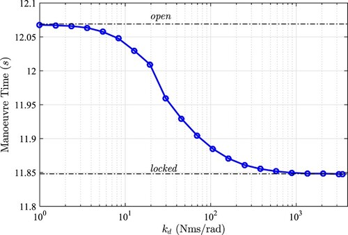
Although the racing vehicle and manoeuvre type considered here are different to that presented in [6], the results are qualitatively similar. As the value of $k_d$ increases, the manoeuvre time approaches a horizontal asymptote, which in this case occurs at t = 11.848s. The section which follows addresses whether further performance improvement can be gained from varying the torque bias strategy along the manoeuvre distance.

3.2. Optimal LSD solution

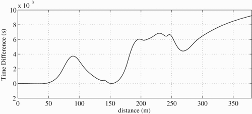
The manoeuvre times and vehicle trajectory curvatures for open, locked and optimal LSD differentials are shown in Table 5 and Figure 5 (a).The time difference between locked and open solutions is significant, at 0.22s. This has been shown to be due to the vehicle's increased braking and acceleration capability [1] when operating with a locked driven axle. This is confirmed in the velocity trace shown in Figure 6 (a), in which the locked differential vehicle is able to brake approximately 10 m later (at 55 m) and starts to accelerate over 10 m earlier (at 200 m) than the open differential. The time difference between locked and optimal LSD configurations is less pronounced however, at 0.01  s.¹ Although this seems like a relatively small performance gain, this difference may start to become more significant over a race distance. To understand where the differences between these two configurations lie, the time difference when projected along the track centreline is shown in Figure 7. This illustrates that the majority of the gain is generated at two key points in the manoeuvre, at 150–180 m and 260–380 m.

Figure 5. (a) Lane change vehicle trajectory curvature (open, locked and optimal LSD configurations shown) (b) slipping/locked status and trajectory of optimal LSD configuration.

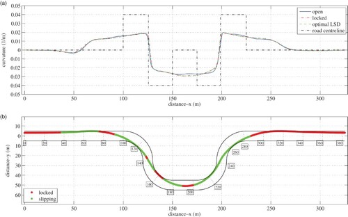
Table 5. Lane change manoeuvre time summary.

	Open	Locked	Optimal LSD
Time (s)	12.069	11.848	11.839

On track, the first of these points (150–180 m) corresponds to where the vehicle is changing directions (from right to left), whilst still under braking. Assessment of the total propulsive/brake torque in Figure 6(c) and 6(d) confirms that the optimal LSD is able to brake less and maintain a slightly higher entry speed in this region. At the second point, between 260 and 380 m, the vehicle is exiting the last corner of the lane change onto a straight. Again, a higher propulsive torque (see Figure 6(d)) is maintained, allowing a higher exit speed to be achieved. This also corresponds to a reduction in the peak steering angle just before this point at 250 m (see Figure 6(b)).

Figure 6. (a) Absolute speed ($\sqrt{U^2+V^2}$) (b) steering angle, δ (c) total propulsive/braking torque, ${\gamma }_t$ (d) total propulsive/braking torque - closeup (e) yaw rate, r, (f) yaw rate - closeup.

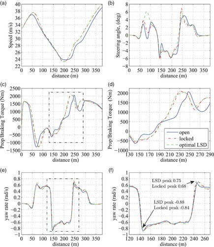
Figure 7. Locked - optimal LSD time difference.

Further insights can be gained by considering the yaw response of the vehicle when fitted with an LSD (when compared to a locked differential). Inspection of Figure 6(e) and 6(f) show the peak yaw rates in these two key phases. Although the difference is small, the optimal LSD is able to provide a higher peak yaw rate at both 145 and 245 m. This has provided a more agile vehicle during the demanding direction changes, turned the vehicle into the corner quicker and allowed a small time advantage. In terms of the racing line curvature, there is a small difference between open and locked configurations (see Figure 5(a)). The open configuration is shown to encourage a slightly earlier entry to the first corner at 120m, so that a larger radius (i.e. smaller curvature) can be maintained at the subsequent corner at 175 m. This has allowed a slightly higher apex speed of 23.7 m/s to be achieved which is +0.6 m/s when compared to locked and LSD configurations (see Figure 6(a)).

The driven wheel speed difference and torque bias of the optimal LSD solution are detailed in Figure 8(a) and 8(b). These are related to the track in Figure 5 (b), which shows the slipping/locked status throughout the manoeuvre. The locked state is defined as the condition when $|{\omega }_3-{\omega }_4|<0.1$ rad/s.

Figure 8. (a) driven wheel speed difference (${\omega }_3-{\omega }_4$) (b) optimal torque bias $T_b=\frac{1}{2}(T_3-T_4)$ (LSD only).

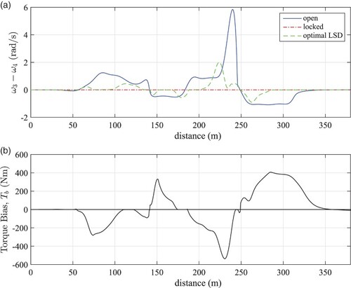
It is interesting to note that the torque bias magnitude (Figure 8(b)) typically reduces to near-zero for a period, close to the apex points of the manoeuvre (specifically at 120, 175 and 245 m). In terms of the torque bias direction, this obeys the convention described in [1]. Under braking conditions into the first right hand corner (at 65 m), the inner wheel is rotating slower than the outer. It is also more lightly loaded and more likely to lock than the outer driven wheel. The wheel speed difference is therefore positive (${\omega }_3>{\omega }_4$), encouraging an outer to inner wheel (understeer) torque bias where $T_3<T_4$. Conversely, during the exit of the last right hand corner at 260 m, the inner wheel has started to overspeed the outer (${\omega }_3<{\omega }_4$), since this lightly loaded inner wheel is now attempting to longitudinally accelerate the vehicle. The resulting torque bias direction has thus switched signs ($T_3>T_4$) providing an oversteer moment.

4. Tyre wear

Although not documented in literature, it is well known in the motorsport industry that in certain instances, a locked differential typically brings with it increased levels of tyre wear. This has particular significance when considering vehicle lap times over a race distance, as peak tyre forces gradually degrade with extended use. These factors must be borne in mind when considering any potential LSD configuration, particularly when the torque bias magnitude is high.

The creation of quantitative tyre wear models is a complex task and is currently a highly active area of research [19,20]. Accurate tyre wear predictions over a typical race distance are important since they help race teams to make tactical decisions regarding race-strategy. In this analysis, the qualitative approach proposed in [20] is used to demonstrate the potential of LSD configuration to influence tyre wear. The rate of tyre wear $W_r$, can be described as the amount of rubber lost from a unit surface per tyre revolution. A common assumption is that this is proportional to the amount of frictional work $W_f$, performed by the tyre [19,20]. The wear rate can be described by the expression: (67) $W_r=A_b{W}_f,$(67) where $A_b$ is an abradability factor, defined as the amount of rubber lost per unit area, per unit frictional work. This depends on many factors, including the rubber compound and carcass construction, as well as the road surface smoothness, tyre temperature and any interfacial contaminants (water e.g.) between the tyre-road contact [20,21]. For this comparative, qualitative analysis, its value is held constant. The focus instead, is placed on the frictional work generated by the longitudinal slip of the driven wheels. This can be defined as [20]: (68) $W_f={\int }_{s_i}^{s_f}|F_x\kappa |\frac{F_z}{F_{z_{\mathrm{ref}}}}\mathrm{d}s,$(68) where $F_{z_{\mathrm{ref}}}$ is a reference normal load and $s_i$ and $s_f$ are the start and end distance of the manoeuvre. Thus, the total frictional energy developed at the rear (driven) axle is: (69) $W_{f_{\mathrm{rear}}}={\int }_{s_i}^{s_f}|F_{x3}{\kappa }_3|\frac{F_{z3}}{F_{z_{\mathrm{ref}}}}\mathrm{d}s+{\int }_{s_i}^{s_f}|F_{x4}{\kappa }_4|\frac{F_{z4}}{F_{z_{\mathrm{ref}}}}\mathrm{d}s.$(69) This expression can be thought of as the longitudinal frictional wear energy (units in kJ) generated when developing longitudinal tyre forces.

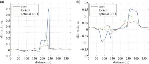
Referring back to Section 3.2, the frictional energy developed at the rear axle for open, locked and optimal LSD configurations during the lane change manoeuvre is shown in Figure 9. The only perhaps surprising result is the total optimal LSD tyre wear energy (33.7 kJ) is over 6.5% more than that of the locked configuration (31.6   kJ), by the end of lane change. Inspection of the wear energy history in Figure 9 reveals that up until 225m, the locked differential actually generated the most wear energy. At this point, a combination of a low normal force on the inside wheel and the need to accelerate out of the corner has promoted excessive longitudinal slip on this inside wheel (in the open and optimal LSD cases). Figure 10(a) and 10(b) demonstrate the longitudinal slip ratios of the two rear wheels. It is clear that the optimal LSD has a reduced peak slip during this phase, when compared to the open differential. Nevertheless, the sudden increase in longitudinal slip between 200 and 250  m has caused a dramatic rise in wear energy at this point in the manoeuvre. It should be noted that analysis of the wear energy over a full lap distance is required to confirm if these results are representative of longer more complex manoeuvres.

Figure 9. Total driven wheel tyre wear energy, $W_{f_{\mathrm{rear}}}$.

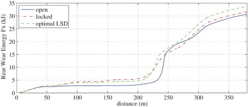
Figure 10. (a) rear left slip ratio ${\kappa }_3$ (b) rear right slip ratio ${\kappa }_4$.

5. Stability and controllability

LSD setup has been shown to have a significant influence on vehicle stability and controllability [1]. To compare the influence of LSD strategy on these important handling traits, stability derivatives are employed [12,22]. These consider the resultant change in yaw moment (N or the right hand side of Equation (3(3) $\begin{array}{rl}{J}_z\dot{r}& =(\cos \delta (F_{x1}-F_{x2})-\sin \delta (F_{y1}+F_{y2}\left)\right)\frac{w}{2}+(F_{x3}-F_{x4})\frac{w}{2}\\ & +a(\sin \delta (F_{x1}+F_{x2})+\cos \delta (F_{y1}+F_{y2}\left)\right)-b(F_{y3}+F_{y4})\end{array}$(3) )), when small perturbations are applied to a linearised vehicle model. Although these have traditionally been applied to the steady state case, they have also been used under transient conditions [3,12]. The key assumption made, is that the response to small inputs will give representative metrics for limit behaviour. This is particularly relevant in the racing vehicle case, where the driver is concerned with how the vehicle reacts to small steering and throttle inputs at the acceleration limits. Furthermore, it is this response that will ultimately determine how much of the performance envelope can be extracted.

Alternative approaches which give a more complete nonlinear description of system stability are typically based on phase plane and bifurcation methods [23]. Significant insight can be gained from these techniques, but it can be difficult to visualise how stability and controllability metrics change during a transient manoeuvre, where the vehicle speed and control inputs are continually changing. It is for this reason that stability derivatives have been adopted in this work.

In this analysis, perturbation of side slip angle β (where $\beta =\arctan \left(V/U\right)$) and the steering angle δ are considered. More formally, these can be described as the relative yaw stiffness $N_{\beta }$ and control derivative $N_{\delta }$ where : (70) $N_{\beta }=\frac{\mathrm{\partial }N}{\mathrm{\partial }\beta },$(70) (71) $N_{\beta }{N}_{\delta }=\frac{\mathrm{\partial }N}{\mathrm{\partial }\delta }.$(71) In practical terms, when the yaw stiffness is positive, there is an understeer moment acting on the vehicle which attempts to return the vehicle to the straight ahead position. When negative, the yaw moment is acting to increase the side slip angle, and hence increase levels of oversteer [12]. It should be noted that although negative yaw stiffness invariably leads to a more unstable vehicle, it does not by itself define the boundary of instability. The control derivative defines the driver's ability to influence the direction of the vehicle, so can be thought of as a control power or ‘turn-in’. When this falls to zero, the driver no longer has any control of the vehicle through the steering. In general terms, an increase in yaw stiffness increases the stability of the vehicle while reducing the associated controllability.

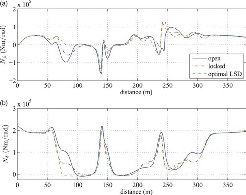
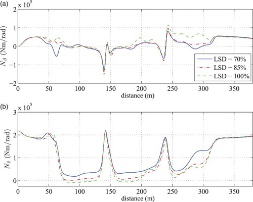
The yaw stiffness and control derivatives have been generated for the lane change manoeuvre described in Section 3.2 and are depicted in Figure 11(a) and 11(b). The most significant difference is seen during the corner entry phase at 80 m. In this region, the optimal LSD yaw stiffness remains close to zero, whilst the locked and open configurations decrease further to $-0.5\times {10}^5$ and $-1.0\times {10}^5$ Nm/rad, respectively. There is further evidence of improved vehicle stability, demonstrated by the steering traces in Figure 6 (b). The less oscillatory nature of the optimal LSD steering suggests that driver workload has been reduced during this braking and turn-in phase of the manoeuvre. The increase in vehicle stability however, has been met with an associated reduction in the controllability, as indicated by the control derivatives in Figure 11 (b).

Figure 11. (a) Yaw stiffness, $N_{\beta }$ (b) control derivative, $N_{\delta }$.

6. Influence of road-tyre friction

To investigate the effect of varying friction levels on track, the same lane change manoeuvre was conducted with the longitudinal and lateral tyre forces scaled down by 15 % and 30%. The intention was to replicate intermediate (greasy) and totally wet track conditions. This was achieved through the scaling factors in Equations  (33(33) $D_x=(p{D}_{x1}+p{D}_{x2}\mathrm{d}{f}_z){\lambda }_{\mu ,x}$(33) ) and (38(38) $D_y=(p{D}_{y1}+p{D}_{y2}\mathrm{d}{f}_z){\lambda }_{\mu ,y}$(38) ) where ${\lambda }_{\mu ,x}={\lambda }_{\mu ,y}$ = 0.85 (intermediate) and ${\lambda }_{\mu ,x}={\lambda }_{\mu ,y}$ = 0.70 (wet). It should be noted, that in the case of wet conditions, a non-hydroplaning tyre-road contact is assumed. The resulting manoeuvre times and control histories of the optimal LSD configuration are shown in Table 6 and Figure 12(a)–(d).

Figure 12. (a) Absolute speed ($\sqrt{U^2+V^2}$) (b) steering angle, δ (c) total propulsive/braking torque, ${\gamma }_t$ (d) optimal torque bias $T_b=\frac{1}{2}(T_3-T_4)$.

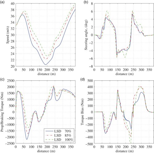
Table 6. Lane change manoeuvre time summary – variable road friction.

Friction level	100% (dry)	85% (inter)	70% (wet)
Time (s)	11.839	12.313	13.165

As one might expect, the speed histories in Figure 12(a) show that as track conditions deteriorate, the vehicle must brake sooner and reduce its associated minimum apex speed. This has reduced by over 3 m/s between dry and fully wet conditions. Interestingly, at a 70% grip level, the torque bias (Figure 12(d)) is seen to increase under braking (between 50 and 100  m), but decrease under acceleration (between 180 and 320  m). Referring to the stability derivatives depicted in Figure 13(a) and 13(b), these regions also show significant reductions in yaw stiffness (specifically at 65 , 200 and 275 m). For the reasons outlined in Section 3.2, differential yaw moments generated under braking typically stabilise the vehicle with an understeer moment. Under acceleration however, this moment switches direction to oversteer. A conclusion that can be drawn from the specific case considered, is that as friction levels reduce, torque biases which encourage understeer moments under braking, but reduce oversteer moments under acceleration, are more likely to provide optimal LSD characteristics.

Figure 13. (a) Yaw stiffness, $N_{\beta }$ (b) control derivative, $N_{\delta }$ (reduced road friction).

7. Conclusions

This paper has described a minimum time optimal control method for determining the ideal torque biasing profile of an LSD. A RWD racing saloon racing vehicle was considered, carrying out a traditional lane change manoeuvre. The optimal LSD was shown to give 0.2s advantage over an open differential and 0.01s when compared to a locked differential (over a 380 m long manoeuvre).

The performance gain of the optimal LSD was related to the phases of the manoeuvre which required a quick direction change, due to the increased peak yaw rate the optimal LSD was able to provide. One can conclude therefore, that on tight, twisty circuits the optimal LSD profile will be most beneficial. The work also highlights the need to consider transient vehicle behaviour in quantifying the influence of certain vehicle tuning parameters on the minimum time solution.

The method outlined in this paper can be used to find both optimal passive LSD characteristics (for torque or speed sensing differentials e.g.), or in the formulation of a semi-active control algorithm.

Disclosure statement

No potential conflict of interest was reported by the authors.

Additional information

Funding

The authors gratefully acknowledge the support of the UK Engineering and Physical Sciences Research Council [grant numbers EP/I037792/01 and EP / 10001219] and Xtrac Ltd.

Notes

1. Differences of this magnitude should always be compared to the numerical resolution of the approach, to ensure gains are related to the vehicle performance. In this case, the magnitude of the penalty cost in comparison to the manoeuvre time was below 2.0%. The difference in penalty cost between locked and optimal LSD solutions was found to be one order of magnitude smaller than the difference in manoeuvre time.

References

- Tremlett A, Assadian F, Purdy D, Vaughan N, Moore A, Halley M. Quasi steady state linearisation of the racing vehicle acceleration envelope: a limited slip differential example. Vehicle Syst Dyn: Int J Vehicle Mech Mobil. 2014.
- Brayshaw D. The use of numerical optimisation to determine on-limit handling behaviour of race cars. [PhD thesis], Department of Automotive, Mechanical and Structural Engineering, Cranfield University; 2004.
- Kelly DP. Lap time simulation with transient vehicle and tyre dynamics. [PhD thesis], Cranfield University, School of Engineering, Automotive Studies Group; 2008.
- Wright P. Formula 1 Technology. Warrendale, PA: Society of Automotive Engineers (SAE); 2001, p86.
- FIA technical regulations [cited 2013 June 3], Available from: www.fia.com/sport/regulations.
- Perantoni G, Limebeer DJ. Optimal control for a formula one car with variable parameters. Vehicle Syst Dyn. 2014.
- Timings JP, Cole DJ. Minimum manoeuvre time calculation using convex optimization. J Dyn Syst Meas Cont. 2013;135.
- Casanova D, Sharp RS, Symonds P. Minimum time manoeuvring: the significance of yaw inertia. Vehicle Syst Dyn. 2000;34:77–115. doi: 10.1076/0042-3114(200008)34:2;1-G;FT077
- Tavernini D, Massaro M, Velenis E, Katzourakis DI, Lot R. Minimum time cornering: the effect of road surface and car transmission layout. Vehicle Syst Dyn. 2013;51:1533–1547. doi: 10.1080/00423114.2013.813557
- Pacejka HB. Tyre and vehicle dynamics. Oxford: Butterworth Heinemann; 2002.
- Bryson AE, Ho Y. Applied optimal control: optimization, estimation and control. Abingdon, Oxon: Taylor and Francis; 1975.
- Milliken WF, Milliken DL. Race car vehicle dynamics. Warrendale, Pa: SAE; 1995.
- Tavernini D, Velenis E, Lot R, Massaro M. The optimality of the handbrake cornering technique. ASME J Dyn Syst Meas Cont. 2014;136:041019-1--041019-11.
- Bertolazzi E, Biral F, Da Lio M. Symbolic-numeric efficient solution of optimal control problems for multibody systems. J Comput Appl Math. 2006;185:404–421. doi: 10.1016/j.cam.2005.03.019
- Betts X. Practical methods for optimal control and estimation using nonlinear programming. Philadelphia: Society for Industrial and Applied Mathematics (SIAM); 2001.
- Pesch HJ. A practical guide to the solution of real-life optimal control problems. Cont Cybern. 1994;23(1/2):7–60.
- Bertolazzi E, Biral F, Da Lio M. Real-time motion planning for multibody systems. Multibody Syst Dyn. 2007;17:119–139. doi: 10.1007/s11044-007-9037-7
- Massaro M, Cole DJ. Neuromuscular-steering dynamics: motorcycle riders vs car drivers. ASME Dynamic Systems and Control Conference, 2012 October 17–19, Fort Lauderdale, FL; 2012.
- Knisley S. A correlation between rolling tire contact friction energy and indoor tread wear. Tire Sci Technol. 2002;30(2):83–99. doi: 10.2346/1.2135251
- Da Silva MM, Cunha RH, Neto AC. A simplified model for evaluating tire wear during conceptual design. Int J Auto Tech. 2012;13(6):915–922. doi: 10.1007/s12239-012-0092-6
- Veith AG. The most complex tire-pavement interaction: tire wear. ASTM Special Technical Publication. 1986;929:125–158.
- Radt H, Van Dis D. Vehicle handling responses using stability derivatives. SAE Technical Paper 960483; 1996. doi:10.4271/960483.
- Yi J, Li J, Lu J, Liu Z. On the stability and agility of aggressive vehicle manoeuvres: a pendulum-turn manoeuvre example. Control Systems Technology, IEEE Transactions. 2012;20(3):663–676. doi: 10.1109/TCST.2011.2121908