Using inerter-integrated absorbers to improve the performance of an in-wheel motor system

Abstract

The in-wheel motor (IWM) is a promising advancement in electric vehicle propulsion since it offers greater packaging efficiency and torque vectoring capabilities than a chassis-mounted motor. However, the increased unsprung mass degrades the vehicle dynamics by increasing body vertical acceleration (BVA) and tyre dynamic load (TDL), worsening ride comfort and road-holding respectively. Another important consideration is magnetic gap deformation (MGD), which results from the deflection between the motor stator and rotor. Reducing MGD improves the motor reliability and longevity. This paper addresses these issues by incorporating inerters into an existing IWM model. They are incorporated into the strut and bushes to control BVA, TDL and MGD. The system optimised for MGD resulted in a deflection reduction of over 98% without compromising performance of the other indices. Optimising the strut and bushes for BVA and TDL reduced them by 20% and 9% respectively without degrading MGD. A sensitivity analysis of the results is presented. Here the damping and inertance values are varied by 20% from the optimum, and the resulting performance still improves upon the default. It is concluded that there are significant potential improvements where inerters are included in an in-wheel motor system.

Keywords:

• Inerter-integrated absorber
• in-wheel motor
• ride comfort
• tyre dynamic load
• magnetic gap deformation

1. Introduction

In recent years, increasing greenhouse gas emissions and pressure to reduce these, has led to the renewed interest in electric vehicles (EVs). With transport estimated to contribute to 14% of global ${\text{CO}}_2$ emissions annually [1], this is clearly a valid step to a net carbon neutral future.

Traditionally, an EV is created by mounting the electric motor to the sprung mass (the chassis or body) and driving the wheels through regular driveshafts. Such propulsion methods can be referred to as chassis-mounted motors, and are similar in principle to the internal combustion engine. The alternative method for powering an EV is through use of an in-wheel motor (IWM). The IWM is not a new proposition. For example, the first IWM patent was filed for in 1884 [2], and the first IWM powered vehicle was the Lohner-Porsche in 1900 [3].

There are two main types of IWM: inner rotor and outer rotor. The outer rotor type is direct drive, and hence is simpler and more robust than the inner rotor type, (which requires a reduction gear) [4]. However, the outer rotor type is often heavier and larger than the inner rotor type [4]. Due to the simplicity and robustness, the outer rotor IWM is generally the more common form of IWM. Hence this design is considered here; however the methodology applied in this study is applicable to either rotor type.

The IWM provides a number of benefits over the chassis-mounted motor. These include improved drivetrain efficiency, due to the removal of driveshafts, and more effective torque vectoring mechanisms [3]. Similarly, it also allows for a greater packaging efficiency, which leads to greater space inside the vehicle [3]. However, the main disadvantage of the IWM is the resulting increase in unsprung mass for the vehicle. This additional unsprung mass is linked to worsening system dynamics and driveability characteristics [5,6]. Hence it is key to reduce these undesirable characteristics through the design or optimisation of the IWM system.

Since the IWM was first proposed, multiple papers have considered modelling the IWM [7], for example suggesting novel designs to counteract some of the known drawbacks [8–12]. Authors have also investigated active control of the suspension architecture to counteract the negative effects of the IWM on system dynamics [13–16]. The novel designs previously suggested include reducing the unsprung mass. This was achieved by reducing the size of the motor body itself to the minimum possible volume, given a performance standard [8]. Other papers have considered moving the mass of the stator to the sprung mass [11,12], and isolating the stator and rotor from the system using rubber bushes [9,10]. In addition [10] provides a sensitivity analysis through a relative percentage change in optimised stiffness, damping and mass parameters. This approach to sensitivity will also be adopted in Section 5 of this paper.

An important factor when considering the IWM is the magnetic gap deformation (MGD), which is defined as the relative deflection between the rotor and stator of the motor. The deflection between rotor and stator can lead to an unbalanced radial magnetic force. This acts as a destructive input to the system in addition to the existing road input [17]. This study uses a simplified modelling strategy where the effect of the radial magnetic force is neglected, and all parameters are considered linear (as in [10]). Reductions of MGD have been considered in the past. For example, Luo and Tan [9] found that isolating the rotor and stator of the motor from the unsprung and sprung masses respectively can result in a reduction in MGD in comparison to a traditional three mass model (their novel IWM model uses five masses). This paper will build on their rubber bush solution by incorporating inerter-based absorbers into the suspension strut and bushes.

The inerter is a recently introduced passive mechanical device which is the mechanical equivalent of an electrical capacitor [18]. It provides a force which is proportional to the relative acceleration between its two endpoints. The inerter is often constructed mechanically as a flywheel-based device [18] or a ball-screw device [19]. The inerter can also be constructed hydraulically as a fluid inerter [20,21]. These construction methods permit the inerter to provide much higher inertance values than its mass, thereby affecting the magnitude and phase of the system dynamics. As a result, the inerter has been incorporated in a variety of industries such as automotive [19,22], civil [23,24] and railway [25–27] applications, but as of yet has not been incorporated into the IWM system.

The Hall-Bush fluid integrated bush has been incorporated into railway vehicles for a number of years [25]. This is often modelled as a damper in parallel and series with a spring [25]. In addition to this, Lewis et al. [25] suggests an inerter-integrated bushing device for use in railway vehicles which is shown to outperform the traditional Hall-Bush device. Therefore building on the work of Lewis et al. [25], a similar concept is proposed and numerically assessed in this paper to be used in an automotive IWM application.

With the introduction of the inerter, a complete force-current analogy between the mechanical and electrical domains can be obtained. Therefore, the network synthesis theories, which were originally developed for electrical systems, can be directly applied to any mechanical system. This has extended the range of possible absorber candidates and their ability to affect the dynamics of the system. To facilitate this, the structure-immittance approach was introduced by [28]. The structure-immittance approach takes a fixed number of springs, dampers and inerter elements in an absorber layout and proposes a set of generic absorber networks. These generic absorber networks yield a transfer function, which can be simplified to give any form of absorber network an individual transfer function. It is therefore extremely useful where multiple absorber layouts are considered and then optimised, such as in this study. This approach has already been used successfully in an automotive context, and hence is suitable for this application [29].

Using the structure-immittance approach and generating a selection of inerter-based absorber networks can give larger performance improvements than is possible with a more traditional parallel inerter. For example, [30] states that, for a racing car (a vehicle with stiffer suspension springs), inerters can only provide 10–20% ride comfort improvement in a quarter-car suspension model. When the spring stiffness is reduced to that of a road car, the performance improvements are negligible. Smith and Wang [22] found that using inerter-based networks, the performance improvement would increase with increasing spring stiffness, thus reinforcing the conclusions made in [30]. Similarly, Zhang et al. [29] found that the ride comfort improvement could be as high as 14.8% for a typical road car when using inerter-based networks. This is another way in which the structure-immittance approach is a useful tool to yield greater performance improvements in vehicle suspension.

This paper will explore a fully passive vibration absorbing system for an IWM, in which inerters are incorporated into the dynamic vibration absorbers. These inerters will be incorporated into the suspension strut as well as the bushes. Hence, this allows for the consideration of the key issues inherent to the IWM system (worsened ride comfort and road-holding), as well as the focus on reducing MGD, using an entirely passive absorber method.

Section 2 will introduce the model used to represent the IWM here, the objective functions and constraints used in the analysis, and consider the optimisation methods used. Section 3 presents the optimisation of the system to reduce MGD, and hence improve the IWM reliability and longevity. Section 4 then follows this to show how the vertical dynamics of the vehicle can be improved, through reducing the body vertical acceleration and tyre dynamic load. Section 5 will then explore the sensitivity of the optimised solutions, before conclusions are presented in Section 6.

2. In-wheel motor model, performance indices and methodology

2.1. In-wheel motor model introduction

As previously mentioned, the IWM type studied here is the outer rotor type. The model used in this study differs from a traditional IWM model since the stator and the rotor are suspended on rubber bushes instead of rigidly fixed to the wheel hub and rim respectively. These rubber bushes have been shown, in [9], to reduce the relative displacement between the rotor and stator (i.e.: the MGD). This MGD can act as an additional source of excitation in addition to the road input ($x_0$), since it promotes a nonlinear unbalanced radial magnetic force as discussed by [17]. Therefore it is beneficial to reduce or constrain MGD (as will be discussed further in Section 2.3) to prevent this unbalanced radial magnetic force.

The traditional rubber bushes and suspension strut can be modelled as a spring and damper in parallel; however, as will be explored in Section 3.1, an inerter-based absorber will replace the pure damper. As a result, they are modelled using a spring in parallel with a generic network. This can be seen in Figure 1, (with the parameters and their values described in Table 1). The parameters and this model (and the potential limitations) are discussed further in Section 2.2.

The generic networks discussed previously represent the force-velocity structural-immittances of an absorber network (termed ‘admittance function’), using an approach first derived by [28] (a more complete description thereof is provided in Appendix A). It is this force-velocity admittance which permits a full range of alternatives to the dampers in the original model to be considered. For the purposes of this study, a maximum of three elements will be considered in each case consisting of one inerter, one damper and one spring. These eight networks can be seen in Figure 2 (III-1 to III-8). Figure 2 also includes a damper strut (I-1) which represents the baseline. The main reason for using generic networks, rather than deriving the equations of motion each time, is one of simplicity and ease; simply changing a transfer function allows multiple layouts to be easily considered in a single optimisation.

Figure 1. IWM model used in this study, adapted from [9].

Table 1. IWM parameter values and description, reproduced from [9].

Parameter	Value	Description
$m_1$	60 kg	Mass of tyre and wheel rim (unsprung mass)
$m_2$	420 kg	Vehicle body sprung mass
$m_{31}$	20 kg	Mass of wheel hub and brake calliper
$m_{32}$	30 kg	Stator mass
$m_{33}$	20 kg	Rotor mass
$k_1$	400 kN/m	Tyre stiffness
$k_2$	80 kN/m	Main suspension strut stiffness
$k_{31}$/$k_{32}$	5 kN/m	Stiffness of bushes
$k_{41}$/$k_{42}$	5 MN/m	Bearing stiffness
$H(s)$	–	Suspension strut generic network
$G(s)$	–	Generic network for the bush between stator and hub
$Y(s)$	–	Generic network for the bushes between rotor and wheel rim

Figure 2. The absorber layouts tested, derived using the structure-immittance approach [28].

It is important to keep the overall static stiffness of the system the same. This is because the static stiffness defines the performance and response of the vehicle. For example, a stiffer spring corresponds to heavy goods vehicles, and a softer spring to more comfort-orientated vehicles [31]. Therefore, in order to ensure the system remains comparable before and after any optimisation, the static stiffness will remain fixed throughout. It is for this reason that only the dampers are replaced by generic networks. This also means that layouts III-1 and III-8 (Figure 2) will have their stiffness (k) fixed to zero during any optimisation. As their stiffnesses are parallel to their damping and inertance, it would therefore sum with the fixed static stiffness of the system and change it.

The equations of motion for the system are written in matrix form as follows: (1) $\begin{array}{rl}& \left[\begin{array}{ccccc}{m}_1& 0& 0& 0& 0\\ 0& m_2& 0& 0& 0\\ 0& 0& m_{31}& 0& 0\\ 0& 0& 0& m_{32}& 0\\ 0& 0& 0& 0& m_{33}\end{array}\right]\left[\begin{array}{c}{\ddot{x}}_1\\ {\ddot{x}}_2\\ {\ddot{x}}_{31}\\ {\ddot{x}}_{32}\\ {\ddot{x}}_{33}\end{array}\right]+\left[\begin{array}{ccccc}y& 0& 0& 0& -y\\ 0& h& -h& 0& 0\\ 0& -h& h+g& -g& 0\\ 0& 0& -g& g& 0\\ -y& 0& 0& 0& y\end{array}\right]\left[\begin{array}{c}{\dot{x}}_1\\ {\dot{x}}_2\\ {\dot{x}}_{31}\\ {\dot{x}}_{32}\\ {\dot{x}}_{33}\end{array}\right]\\ & +\left[\begin{array}{ccccc}{k}_1+k_{32}+k_{41}& 0& -k_{41}& 0& -k_{32}\\ 0& k_2& -k_2& 0& 0\\ -k_{41}& -k_2& k_2+k_{31}+k_{41}& -k_{31}& 0\\ 0& 0& -k_{31}& k_{31}+k_{42}& -k_{42}\\ -k_{32}& 0& 0& -k_{42}& k_{32}+k_{42}\end{array}\right]\left[\begin{array}{c}{x}_1\\ x_2\\ x_{31}\\ x_{32}\\ x_{33}\end{array}\right]=\left[\begin{array}{c}{k}_1{x}_0\\ 0\\ 0\\ 0\\ 0\end{array}\right]\end{array}$(1) where all terms are as previously defined.

The force-velocity immittances of the absorber layouts discussed are defined in the Laplace domain. As a result, they cannot be directly placed into time domain equations of motion. In the matrix equation of motion (Equation  (1(1) $\begin{array}{rl}& \left[\begin{array}{ccccc}{m}_1& 0& 0& 0& 0\\ 0& m_2& 0& 0& 0\\ 0& 0& m_{31}& 0& 0\\ 0& 0& 0& m_{32}& 0\\ 0& 0& 0& 0& m_{33}\end{array}\right]\left[\begin{array}{c}{\ddot{x}}_1\\ {\ddot{x}}_2\\ {\ddot{x}}_{31}\\ {\ddot{x}}_{32}\\ {\ddot{x}}_{33}\end{array}\right]+\left[\begin{array}{ccccc}y& 0& 0& 0& -y\\ 0& h& -h& 0& 0\\ 0& -h& h+g& -g& 0\\ 0& 0& -g& g& 0\\ -y& 0& 0& 0& y\end{array}\right]\left[\begin{array}{c}{\dot{x}}_1\\ {\dot{x}}_2\\ {\dot{x}}_{31}\\ {\dot{x}}_{32}\\ {\dot{x}}_{33}\end{array}\right]\\ & +\left[\begin{array}{ccccc}{k}_1+k_{32}+k_{41}& 0& -k_{41}& 0& -k_{32}\\ 0& k_2& -k_2& 0& 0\\ -k_{41}& -k_2& k_2+k_{31}+k_{41}& -k_{31}& 0\\ 0& 0& -k_{31}& k_{31}+k_{42}& -k_{42}\\ -k_{32}& 0& 0& -k_{42}& k_{32}+k_{42}\end{array}\right]\left[\begin{array}{c}{x}_1\\ x_2\\ x_{31}\\ x_{32}\\ x_{33}\end{array}\right]=\left[\begin{array}{c}{k}_1{x}_0\\ 0\\ 0\\ 0\\ 0\end{array}\right]\end{array}$(1) )), the terms h, g and y refer to the inverse Laplace transform of $H(s)$, $G(s)$ and $Y(s)$ defined as follows: (2) $\begin{array}{rl}h& ={\mathcal{L}}^{-1}\{H(s)\}\\ g& ={\mathcal{L}}^{-1}\{G(s)\}\\ y& ={\mathcal{L}}^{-1}\{Y(s)\}\end{array}$(2) where ${\mathcal{L}}^{-1}$ denotes the inverse Laplace transform and all other terms are as previously defined. The time-domain matrix in Equation  (1(1) $\begin{array}{rl}& \left[\begin{array}{ccccc}{m}_1& 0& 0& 0& 0\\ 0& m_2& 0& 0& 0\\ 0& 0& m_{31}& 0& 0\\ 0& 0& 0& m_{32}& 0\\ 0& 0& 0& 0& m_{33}\end{array}\right]\left[\begin{array}{c}{\ddot{x}}_1\\ {\ddot{x}}_2\\ {\ddot{x}}_{31}\\ {\ddot{x}}_{32}\\ {\ddot{x}}_{33}\end{array}\right]+\left[\begin{array}{ccccc}y& 0& 0& 0& -y\\ 0& h& -h& 0& 0\\ 0& -h& h+g& -g& 0\\ 0& 0& -g& g& 0\\ -y& 0& 0& 0& y\end{array}\right]\left[\begin{array}{c}{\dot{x}}_1\\ {\dot{x}}_2\\ {\dot{x}}_{31}\\ {\dot{x}}_{32}\\ {\dot{x}}_{33}\end{array}\right]\\ & +\left[\begin{array}{ccccc}{k}_1+k_{32}+k_{41}& 0& -k_{41}& 0& -k_{32}\\ 0& k_2& -k_2& 0& 0\\ -k_{41}& -k_2& k_2+k_{31}+k_{41}& -k_{31}& 0\\ 0& 0& -k_{31}& k_{31}+k_{42}& -k_{42}\\ -k_{32}& 0& 0& -k_{42}& k_{32}+k_{42}\end{array}\right]\left[\begin{array}{c}{x}_1\\ x_2\\ x_{31}\\ x_{32}\\ x_{33}\end{array}\right]=\left[\begin{array}{c}{k}_1{x}_0\\ 0\\ 0\\ 0\\ 0\end{array}\right]\end{array}$(1) ) can have the Laplace transform taken to produce the frequency domain equations as follows: (3) $\begin{array}{rl}& {\hat{x}}_1(m_1{s}^2+\mathrm{sY}(s)+[k_1+k_{32}+k_{41}])-{\hat{x}}_0(k_1)-{\hat{x}}_{33}(\mathrm{sY}(s)+k_{32})-{\hat{x}}_{31}{k}_{41}=0\\ & {\hat{x}}_2(m_2{s}^2+\mathrm{sH}(s)+k_2)-{\hat{x}}_{31}(\mathrm{sH}(s)+k_2)=0\\ & {\hat{x}}_{31}(m_{31}{s}^2+s[H(s)+G(s)]+[k_2+k_{31}+k_{41}])-{\hat{x}}_2(\mathrm{sH}(s)+k_2)-\\ & {\hat{x}}_1{k}_{41}-{\hat{x}}_{32}(\mathrm{sG}(s)+k_{31})=0\\ & {\hat{x}}_{32}(m_{32}{s}^2+\mathrm{sG}(s)+[k_{31}+k_{42}])-{\hat{x}}_{31}(\mathrm{sG}(s)+k_{31})-{\hat{x}}_{33}{k}_{42}=0\\ & {\hat{x}}_{33}(m_{33}{s}^2+\mathrm{sY}(s)+[k_{32}+k_{42}])-{\hat{x}}_1(\mathrm{sY}(s)+k_{32})-{\hat{x}}_{32}{k}_{42}=0\end{array}$(3) where $\hat{x}$ denotes the Laplace transformed x, s is the Laplace variable and all other terms are as previously defined. The Laplace transformed equations of motion are preferable for the analysis. This is because they permit usage of the frequency domain objective functions as discussed in Section 2.3.

2.2. Discussions and limitations of chosen model

Any model used in engineering has its own limitations, and it is important to be aware of any. Therefore, in this subsection the limitations of the current model will be discussed, as well as the reasons why this model has been chosen over other potential models.

The model itself is a 5 mass model of an IWM first proposed by Luo and Tan [9], where the stator and rotor masses are isolated from the wheel hub and tyre masses respectively using rubber bushes. It was found that this could improve the performance when compared to the traditional 3 mass IWM model. As an example, performance improvements of BVA were found in Ref. [9] to be 2.55%, and for TDL, 5.76%. Considering the rotor and stator as components separated by a bearing allows consideration of the MGD – something that cannot be done with the 3 mass IWM model. This is because, in the 3 mass IWM model, the road surface roughness leads directly to a worsened MGD, whereas the 5 mass model permits this MGD to be limited firstly by having a bearing between rotor and stator, and secondly by isolating the masses with the bushes [9].

The 3 mass model discussed previously is the simplest common model for the IWM, which is developed from the well-known 2 mass quarter-car model. The relations between quarter-car, traditional IWM model and the 5 mass IWM model used here are shown in Figure 3.

Figure 3. Different methods of modelling an IWM from (a) the simplest quarter-car with an increased unsprung mass, (b) the traditional 3 mass IWM with motor mass, unsprung mass and hub mass combined, and (c) the 5 mass IWM used in this study, modified from [9]. In each case, the parameters are as defined earlier.

All three of the models shown in Figure 3 use the same linear spring approximation to the tyre stiffness. This is a limiting factor to the model, as above 80 Hz tyre carcass resonances occur, which requires a much more complex tyre model [32]. However, as the frequencies primarily associated with ride are defined as being between 0 and 25 Hz [33] this simplistic tyre model approximation is appropriate for this study (indeed, Gillespie [33] found it sufficient for their quarter-car analysis between 0 and 25 Hz).

Bearings $k_{41}$ and $k_{42}$ have stiffness values of 5 MN/m. These very high stiffness values lead to high frequency oscillations, which are outside the ride frequency range of 0–25 Hz. This means that they would not be properly considered given the limitations of the simplified quarter car model, which includes a simplified tyre model. It is therefore important to ensure that any high frequency effects are not considered when optimising for the MGD. This is explored further in Section 2.3. It is important to note that Luo and Tan [9] limited their analysis to 0–25 Hz when showing the performance improvements that the 5 mass IWM model can return when compared to the 3 mass IWM model. Therefore, the approach taken here is in line with that study.

In adopting the 5 mass IWM model developed by Luo and Tan [9], the rather high suspension strut stiffness that they provided is also used. A value of 80 kN/m is much higher than a normal quarter-car strut stiffness (such as the 26.09 kN/m used by Zhang et al. [29]). However, it is important to note the extra mass that the IWM brings, combined with the weight of the batteries required for an electric vehicle. For example, Zhang et al. [29] use sprung and unsprung masses of 250 and 40 kg respectively. Compared to the sprung and (total) unsprung mass for this system which are 420 and 130 kg. As a result, the high stiffness of the suspension strut would be necessary to deal with this extra mass.

2.3. Performance indices

When designing a suspension system, there are many different performance metrics that may be used to define the performance quality. In this study, body vertical acceleration and tyre dynamic load are selected to use as objective functions. These can be described using the work of [22] as follows: (4) $\begin{array}{rl}{J}_1& =2\pi (\mathrm{V\kappa }{)}^{\frac{1}{2}}{\left|\left|s{T}_{{\hat{x}}_0\to {\hat{x}}_2}\right|\right|}_2\end{array}$(4) (5) $\begin{array}{rl}{J}_3& =2\pi (\mathrm{V\kappa }{)}^{\frac{1}{2}}{\left|\left|\frac{1}{s}{T}_{{\hat{x}}_0\to k_1({\hat{x}}_1-{\hat{x}}_0)}\right|\right|}_2\end{array}$(5) where $J_1$ refers to the body vertical acceleration (a ride comfort metric) and $J_3$ the tyre dynamic load (a road-holding metric)¹. Here $T_{\hat{a}\to \hat{b}}$ represents the transfer function between $\hat{a}$ and $\hat{b}$ (the input and output of the transfer function respectively), $x_0$ the road input, V the vehicle velocity and κ the road roughness parameter, $||\cdot |{|}_2$ denotes the standard ${\mathcal{H}}_2$ norm and all other terms are as previously defined. The integrator ($\frac{1}{s}$) term in $J_3$, and differentiator (s) in $J_1$ indicate that they correspond to a relative displacement and acceleration respectively.

An equivalent performance metric for MGD, (termed here as $J_m$ to be more comparable to the accepted $J_1$ and $J_3$ metrics) can also be derived. This can be seen as follows: (6) $J_m={(2\mathrm{\pi V\kappa }(\mathrm{\Delta \omega })\sum _{{\omega }_1}^{{\omega }_2}{\left|\frac{1}{s}{T}_{{\hat{x}}_0\to ({\hat{x}}_{33}-{\hat{x}}_{32})}\right|}^2)}^{\frac{1}{2}}$(6) where $\mathrm{\Delta }\omega$ is the frequency step used in the sum (set as 0.1 rad/s here), ${\omega }_1$ is the low frequency cutoff (0 rad/s or 0 Hz here), ${\omega }_2$ is the high frequency cutoff (50π rad/s corresponding to 25 Hz here), and all other terms are as previously defined. A more thorough derivation – including details about the road profile – can be seen in Appendix B. Road velocity profiles are often assumed to approximate a white noise input [34], and hence the vertical road displacement input ${\hat{x}}_0$ is taken to be integrated white noise.

The reason why $J_m$ (Equation  (5(5) $\begin{array}{rl}{J}_3& =2\pi (\mathrm{V\kappa }{)}^{\frac{1}{2}}{\left|\left|\frac{1}{s}{T}_{{\hat{x}}_0\to k_1({\hat{x}}_1-{\hat{x}}_0)}\right|\right|}_2\end{array}$(5) )) cannot use the more typical ${\mathcal{H}}_2$ norm form is because the ${\mathcal{H}}_2$ norm is an integral from $-\mathrm{\infty }$ to ∞ rad/s. This would therefore include the high frequency effects caused by the stiff bearings. The effect of the high stiffness bearings on $J_1$ and $J_3$ (Equations  (4(4) $\begin{array}{rl}{J}_1& =2\pi (\mathrm{V\kappa }{)}^{\frac{1}{2}}{\left|\left|s{T}_{{\hat{x}}_0\to {\hat{x}}_2}\right|\right|}_2\end{array}$(4) ) and (5(5) $\begin{array}{rl}{J}_3& =2\pi (\mathrm{V\kappa }{)}^{\frac{1}{2}}{\left|\left|\frac{1}{s}{T}_{{\hat{x}}_0\to k_1({\hat{x}}_1-{\hat{x}}_0)}\right|\right|}_2\end{array}$(5) ) respectively) is negligible. This was verified through an equation similar in form to $J_m$ (Equation  (6(6) $J_m={(2\mathrm{\pi V\kappa }(\mathrm{\Delta \omega })\sum _{{\omega }_1}^{{\omega }_2}{\left|\frac{1}{s}{T}_{{\hat{x}}_0\to ({\hat{x}}_{33}-{\hat{x}}_{32})}\right|}^2)}^{\frac{1}{2}}$(6) )), and using a similar method as that discussed in Appendix B. When the range of frequencies considered was limited to between 0 and 25 Hz, there was no difference when compared to the ${\mathcal{H}}_2$ norm form shown in Equations  (4(4) $\begin{array}{rl}{J}_1& =2\pi (\mathrm{V\kappa }{)}^{\frac{1}{2}}{\left|\left|s{T}_{{\hat{x}}_0\to {\hat{x}}_2}\right|\right|}_2\end{array}$(4) ) and (5(5) $\begin{array}{rl}{J}_3& =2\pi (\mathrm{V\kappa }{)}^{\frac{1}{2}}{\left|\left|\frac{1}{s}{T}_{{\hat{x}}_0\to k_1({\hat{x}}_1-{\hat{x}}_0)}\right|\right|}_2\end{array}$(5) ). Therefore, using the ${\mathcal{H}}_2$ norm is deemed appropriate.

The parameter values used in this study can be seen in Table 1. These, along with the linear damping parameters are obtained from [9]. In addition, the vehicle velocity (V = 60 kph) and road surface roughness ($\kappa =5\times {10}^{-7}{\mathrm{m}}^3$/cycle) parameters are obtained from [22]. These parameters can then be used to create the benchmark performance that will be improved upon. The default damping properties for the bushes are taken as 1000 and 5000 Ns/m for the strut. Using these, benchmark performance values are obtained as follows: (7) $\begin{array}{rl}{J}_1& =1.473{\mathrm{m}/\mathrm{s}}^2\\ J_3& =928.5\mathrm{N}\\ J_m& =2.265\mu \mathrm{m}\end{array}$(7) which will be used as constraints in future optimisations.

It is important to note that, in traditional quarter-car analysis, ride comfort, tyre grip and suspension working space (analogous to MGD in this study) are conflicting performance criteria that cannot be improved upon simultaneously. Various studies have noticed this for many decades, for example Bender [35], stated in 1968 that vibration and suspension working space is a trade-off which would need to be optimised.

Despite this, many papers have considered optimising one of these criteria whilst constraining the others. An example of this being Zhang et al. [29], who optimised for ride comfort whilst constraining suspension travel and tyre load. In this study, the performance criteria will be optimised separately, whilst constraining the other criteria (like in [29]). This is in order to avoid arbitrary weighting factors, which would need to be used to describe a trade-off between criteria.

2.4. Methodology for identifying the optimal absorber configurations

When optimising, it is important to ensure a global minimum solution is found. Whilst it is difficult, (or even impossible), to guarantee that a global minimum has been found, there are a number of techniques that can be applied to minimise this risk. Optimisation is undertaken in MATLAB using a ‘cascade’ approach.

The first step of the optimisation uses the ‘particleswarm’ optimisation method, with the initial conditions logarithmically spaced through the boundaries provided to the solver. These optimised solutions are passed to ‘patternsearch’ and then ‘fminsearch’ in turn, with the optimised solution gradually getting finer and closer to a global optimum.

This optimisation method is used to optimise the inertance, damping, and stiffness parameters in the absorbers. In doing so, the global optimum inerter-based absorber can be found. As stated earlier, the structure-immittance approach [28] is used as this permits the absorber layouts to be represented as transfer functions. Therefore, it becomes easier to change the component layout without having to derive the equations of motion for the entire system again.

The first part of the analysis in Section 3 will focus on reducing MGD to improve the motor longevity and reliability. The following section (Section 4) will then consider the performance improvements possible for ride comfort and tyre dynamic load metrics, thereby focussing on the vehicle vertical dynamics.

3. Optimisation to reduce $J_m$

The first optimisation step is to improve the reliability and longevity of the IWM through reducing $J_m$.

3.1. Optimisation of bushes

A modification to the system inspired by the railway Hall-Bush system has been proposed by [25]. This allows for inertance to be included in a system by careful design of the fluid passageways within the bush. The work in that study will be expanded to cover this specific application in the following section.

Figure 1 shows the inclusion of generic absorber networks in the place of the bushings ($G(s)$ and $Y(s)$). Since these bushings surround the motor, they should have the greatest influence on the deflection between rotor and stator. As a result, the initial step to improving the $J_m$ performance is to optimise the bushes, whilst placing constraints on the values of $J_1$ and $J_3$.

To numerically compare the performance benefit possible by incorporating an inerter into the bush, initially just the damper bush is optimised for $J_m$. The results of this can be seen in Table 2. Here the best possible performance improvement is 82.5% over the default if both bushes are optimised. In addition to this 82.5% improvement where both bushes are optimised, Table 2 shows that no improvement is possible where one bush is optimised and the other is kept as default in columns 3 and 4.

Table 2. The results of optimising the bushes for $J_m$ with all constraints applied and compared to the benchmark performance.

Parameter values		Default	Tune $G(s)$		Tune $Y(s)$		Tune $G(s)$ and $Y(s)$
$J_1$ (m/s${}^2$)		1.473	1.473		1.473		1.473
$J_3$ (N)		928.5	928.5		928.5		926.4
$J_m$ (μm)		2.265	2.265	0%	2.265	0%	0.3974	82.5%
	b (kg)	-	-		-		-
	c (Ns/m)	1000	1000		1000		1164
G(s)	k (N/m)	-	-	I-1	-	I-1	-	I-1
	b (kg)	-	-		-		-
	c (Ns/m)	1000	1000		1000		745.1
Y(s)	k (N/m)	-	-	I-1	-	I-1	-	I-1

Notes: Here the bushes are optimised individually and then together. In this stage, only damper bushes are considered to see the maximum performance improvement that can be gained before inerters are included. The corresponding absorber layout for each location is shown numerically.

In Table 3, inerters are incorporated into the bushes, with the three-element layouts considered shown in Figure 2. These results show a far more promising improvement in performance, where over 98% improvement is reported over the default value for MGD. This shows the benefit an inerter can have on a system, as the potential improvement in MGD increases from around 80% with pure damper bushes.

Table 3. The results of optimising the bushes for $J_m$ with all constraints applied and compared to the benchmark performance.

Parameter Values		Default	Tune $G(s)$		Tune $Y(s)$		Tune $G(s)$ and $Y(s)$
$J_1$ (m/s${}^2$)		1.473	1.471		1.473		1.464
$J_3$ (N)		928.5	928.5		922.4		923.3
$J_m$ (μ m)		2.265	2.211	2.37%	0.4806	78.8%	0.04273	98.1%
	b (kg)	-	2071		-		2.833
	c (Ns/m)	1000	1014		1000		1310
G(s)	k (N/m)	-	10,000,000	III-3	-	I-1	636,800	III-7
	b (kg)	-	-		486.2		821.4
	c (Ns/m)	1000	1000		712.1		821.4
Y(s)	k (N/m)	-	-	I-1	501,100	III-3	704,200	III-3

Notes: Here the bushes are optimised individually and then together. In this stage, only inerter bushes are considered to see the maximum possible performance improvement. The corresponding absorber layout for each location is shown numerically.

An interesting point of note is that where only one the damper is optimised in Table 2, there is no performance gain identified over the default whilst ensuring the constraints on $J_1$ and $J_3$ were not violated. However, where inerter integrated bushes are optimised, there is a performance improvement possible over just the damper bushes. This again shows the beneficial performance that inerters bring to a system. It is also interesting to note that where only a single inertance-integrated bush is optimised, the performance improvement does not exceed that where both damper bushes are optimised. Also, where only $G(s)$ is optimised with an inertance-integrated bush, the desired value for stiffness is ${10}^7$ N/m. This is incredibly stiff and indicated that the best layout in this case would likely be a damper and inerter in series, as the very stiff spring approximates a rigid connection.

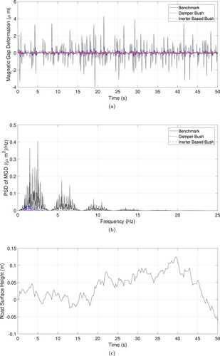
To show this MGD improvement graphically, analysis of the system in the time domain (Figure 4 (a)) is presented. Here the system is excited by a road input generated using the road surface discussed in Section 2.3 and Appendix B, and shown in Figure 4 (c). The power spectral density (PSD) of this response is also shown in Figure 4 (b). Both of these plots show just how comprehensively the optimal inerter-based absorbers are able to reduce the MGD – when compared to either the default or the system with optimal damper bushes.

Figure 4. Comparison of performance for magnetic gap deformation of optimal bushes in(a) the time domain, and (b) the power spectral density of this signal. (c) shows the road surface derived using the method detailed in Appendix B used in these responses.

This step has proven that reducing $J_m$ through optimisation of the bushes alone is possible, and gives excellent results for the reduction of $J_m$. Therefore, the three best performing combinations of inerter-based bushes are taken further (Note: only the single best performing combination of optimal bushes is presented here), and allows all of the parameters to be optimised in a single pass to see if further $J_m$ improvements can be unlocked. This analysis follows in Section 3.2.

3.2. Optimisation of all parameters

Following the success of optimising the bushes for $J_m$, this analysis is built upon by optimising all parameters in a single pass. This means that the parameters in the strut, as well as both bushes, is optimised for $J_m$ at the same time (whilst constraining the values of $J_1$ and $J_3$). The results from this analysis can be seen in Table 4. The results here show an improvement of 98.6% over the default $J_m$ value – an improvement of 0.5% over the optimisation of the bushes alone.

Table 4. The results of optimising all parameters for $J_m$ with all constraints applied and compared to the benchmark performance.

Parameter Values		Default	Optimised for $J_m$ $J_1$, $J_3$ Constrained
$J_1$ (m/s${}^2$)		1.473	1.357
$J_3$ (N)		928.5	928.5
$J_m$ (μ m)		2.265	0.03215	98.6%
	b (kg)	-	447.1
	c (Ns/m)	5000	4988
H(s)	k (N/m)	-	34,380	III-4
	b (kg)	-	6.625
	c (Ns/m)	1000	1859
G(s)	k (N/m)	-	822,800	III-7
	b (kg)	-	935.7
	c (Ns/m)	1000	1156
Y(s)	k (N/m)	-	10,000,000	III-3

Notes: Here the bushes considered are the three best performing combinations of bushes from Section 3.1. The corresponding absorber layout for each location is shown numerically.

The relative lack of improvement (the value for optimised bushes and that for where all parameters are optimised differ by 28.3%) can be explained by looking at the diagram in Figure 1. The bushes surround the stator and rotor, and thus have the best chance to reduce the relative deflection between them. The strut is not directly connected to either of the motor components, and thus cannot affect the force imparted on the stator or rotor as effectively. Therefore, the increase in improvement possible compared to optimising the bushes alone is minimal.

4. Optimisation to reduce $J_1$ and $J_3$

With the knowledge that $J_m$ can be very significantly reduced using inerter-integrated absorbers whilst not degrading the $J_1$ and $J_3$ performance, attention can be paid to the vehicle vertical dynamics metrics, $J_1$ and $J_3$.

4.1. Optimisation of the strut

The first step in improving the $J_1$ and $J_3$ value is to optimise the strut alone. Every layout shown in Figure 2 (including the damper) is considered. When optimising for $J_1$, constraints are placed on $J_3$ and $J_m$. Then, when optimising for $J_3$, constraints are placed on $J_1$ and $J_m$.

The results of the optimisation of the strut for both $J_1$ and $J_3$ can be seen in Table 5. For $J_1$, layout III-4 provided the most optimal performance, and III-3 was best for $J_3$. Whilst it is clear that the inclusion of the inerter provides some performance benefit to the system over a single damper (I-1), the performance gains are minimal – particularly for $J_3$. When the damper alone was optimised, there was no performance improvement over the default for both $J_1$ and $J_3$ whilst not exceeding the value of the constraints. This suggests that the pure damper strut is already optimum, and that any further performance improvements would require an inerter-based absorber in place of the pure damper.

Table 5. The results of optimising the strut for $J_1$ and $J_3$ with all constraints applied and compared to the benchmark performance.

Parameter Values		Default	Optimised for $J_1$ $J_3$, $J_m$ Constrained		Optimised for $J_3$ $J_1$, $J_m$ Constrained
$J_1$ (m/s${}^2$)		1.473	1.365	7.33%	1.466
$J_3$ (N)		928.5	928.5		906.1	2.41%
$J_m$ (μm)		2.265	2.265		2.265
	b (kg)	–	627.9		898.9
	c (Ns/m)	5000	5639		5866
H(s)	k (N/m)	–	0.001020	III-4	1,761,000	III-3

Notes: Here the bushes $G(s)$ and $Y(s)$ are left at their default values, and the percentages represent the percentage improvement between the benchmark and optimised values. Here grey represents a value which has not been optimised, and yellow represents the objective function that is optimised for. The corresponding absorber layout for each location is shown numerically.

One important point to note is the value in each case for $J_m$. For both optimisations the value for $J_m$ is equal to that of the default. This suggests that this constraint plays a key part in limiting the performance of the system.

4.2. Relaxation of ${\mathrm{J}}_{\mathrm{m}}$ constraint

To investigate how important this constraint is, it is relaxed and the resulting performance is analysed. Figure 5 shows the trade-off performance for $J_1$ and $J_3$ where the constraint on $J_m$ is relaxed in 5% intervals. This means that $J_m$ is allowed to exceed the initial constraint by 5%, then 10% and so on to 100%. As a result, the $J_m$ value may increase to twice that of the default. The resulting value for $J_1$ or $J_3$ is then recorded. As a final step, an optimisation is completed where the $J_m$ constraint is completely removed. This does not change the optimum value for $J_1$ and $J_3$ over where the $J_m$ may double that of the default.

Figure 5. Trade-off performance for (a) $J_1$ and (b) $J_3$ optimisation. Here, the constraint on $J_m$ is relaxed from 0% (fully constrained) to 100% (fully unconstrained). Both bushes are dampers in this stage of the analysis.

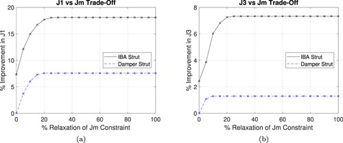
It can be seen in Figure 5 that $J_1$ can improve up to 18% when compared to the benchmark performance, and $J_3$ up to around 7%. It is also clear that even a small reduction in the constraint on $J_m$ can yield a substantial increase in performance for $J_1$ or $J_3$. For example, relaxing $J_m$ by 35% allows $J_1$ to reach its peak performance improvement. At face value, the percentage improvement shown in these results might seem encouraging.

However, relaxation of the $J_m$ constraint is not ideal for two main reasons. Firstly, for the completely removed $J_m$ constraint, a worst case scenario could result in the rotor and stator colliding with each other – with dangerous and costly consequences. Secondly, the more the constraint on $J_m$ is relaxed, the worse the unbalanced radial magnetic force will become, and the more destructive its influence will be [17].

4.3. Optimisation of all parameters

Section 3 considered optimising the system to improve the performance of $J_m$. Here it was shown that over 98% reduction in $J_m$ was possible just through optimising the bushes alone. Therefore, this final optimisation stage aims to show that the limitation on the strut optimisation by the $J_m$ constraint can be reduced by optimising all parameters in a single pass. Combining inertance-integrated bushes with an inerter-based strut will allow for optimisation and improvement in $J_1$ and $J_3$ through the strut, with $J_m$ controlled through the bushes. This will unlock greater improvements in $J_1$ and $J_3$, since the $J_m$ constraint is not so likely to be breached.

Table 6 presents the results where all parameters have been optimised simultaneously for both $J_1$ and $J_3$, (and all constraints applied as normal). One interesting point is that the best performing bush combination is not the same as found in Section 3.1. However, $J_m$ is clearly controlled sufficiently well to allow a much greater performance gain when compared to just optimising the strut. Where everything is optimised, $J_1$ can improve by 20.2% and $J_3$ 9.18%. These values are both better than where the $J_m$ constraint was completely relaxed (Section 4.2), and yet have the advantage of not degrading the performance of $J_m$.

Table 6. The results of optimising all parameters for $J_1$ and $J_3$ with all constraints applied and compared to the benchmark performance.

Parameter Values		Default	Optimised for $J_1$ $J_3$, $J_m$ Constrained		Optimised for $J_3$ $J_1$, $J_m$ Constrained
$J_1$ (m/s${}^2$)		1.473	1.175	20.2%	1.473
$J_3$ (N)		928.5	875.7		843.2	9.18%
$J_m$ (μ m)		2.265	2.265		1.695
	b (kg)	-	226.7		511.1
	c (Ns/m)	5000	2325		4805
H(s)	k (N/m)	-	27,080	III-4	670,800	III-3
	b (kg)	-	97,990		62.34
	c (Ns/m)	1000	2536		505.6
G(s)	k (N/m)	-	150,200	III-3	40,500	III-3
	b (kg)	-	100,000		13.63
	c (Ns/m)	1000	1260		139.3
Y(s)	k (N/m)	-	115,100	III-3	19,380	III-3

Notes: Here the bushes considered are the three best performing combinations of bushes from the previous step (Section 3.1). The corresponding absorber layout for each location is shown numerically.

5. Sensitivity analysis

When constructing a physical device, it is often impossible to guarantee the parameters will match to the optimised values exactly. Over the lifetime of the vehicle for example, components can wear and deviate from their optimised values. This is particularly prevalent in the case of using fluid based devices, (such as the Hall-Bush style hydrobush [25], fluid inerter [20] or viscous damper). This is because fluid viscosities vary with temperature (for a Newtonian fluid [36]), and hence the damping and inertance values will vary in use. Therefore, it is important to carry out a sensitivity analysis to ensure that any optimised performance does not degrade past the default.

This sensitivity analysis is also useful as an approximation to physical testing. Authors such as Wang, et al. have tested physical prototypes of hydraulic inerter using a hydraulic motor [37]. They found that, for larger inertia values of the flywheel attached to the hydraulic motor, expected and experimental inertance could vary by around 22%. This study proposes a linear, network-based methodology to improve the performance of the IWM, and as such physical testing has been left for future studies. However, this sensitivity analysis is intended to approximate the findings of a physical test in a limited way.

In the following sensitivity analyses, the stiffness in each case will remain fixed to the optimised value. The inertance and damping are then varied by a range of $\pm 20\mathrm{\%}$. The inertance and damping values are chosen due to the potential values in viscocities discussed in the previous paragraph.

The strut performance sensitivity analysis is carried out for the case where $J_1$ and $J_3$ are most effectively reduced (i.e.: where all the parameters are optimised in Section 4.3). The bush performance sensitivity analysis is carried out for the best $J_m$ reduction shown in Section 3.1, where the bushes alone were optimised. This section considers the sensitivity of $G(s)$ and $Y(s)$ separately. Sections 5.1 and 5.2 detail these procedures.

5.1. Sensitivity of strut

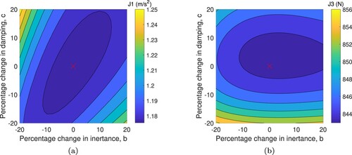
The results of the sensitivity analysis for the strut can be seen in Figure 6. When inertance and damping vary by 20%, the maximum values reported for $J_1$ are 1.256 m/s${}^2$, and for $J_3$ this is 856.3 N. These compare to the optimum performance of 1.175 m/s${}^2$ and 843.2 N respectively. The percentage variation in these parameters from optimum is 6.66% and 1.54% respectively. This indicates that the performance of the optimised system in a ‘worst-case’ scenario will still improve on the performance of the default (1.473 m/s${}^2$ and 928.5 N) by 14.7% and 7.78% respectively, and hence can be considered effective.

Figure 6. Sensitivity performance of the strut for (a) $J_1$ and (b) $J_3$. Both are subject to parameter variation of $\pm 20\mathrm{\%}$ of damping and inertance values from the optimum. Stiffness is fixed at the optimum value. The red cross shows the optimal performance.

5.2. Sensitivity of bushes

The results of the sensitivity analysis for the bushes can be seen in Figure 7. When inertance and damping vary by 20%, the maximum value reported for $J_m$ is 1.068 and 1.051 μm for $G(s)$ and $Y(s)$ respectively. These compare to the optimum performance of 0.04273 μm . The percentage variation in these parameters from optimum is 185% and 184% respectively. These values show that the bushes are far more sensitive to parameter variation than the strut.

Figure 7. Sensitivity performance of (a) $G(s)$ and (b) $Y(s)$ for $J_m$ subject to parameter variation of $\pm 20\mathrm{\%}$ of damping and inertance values from the optimum. Stiffness is fixed at the optimum value. The red cross shows the optimal performance.

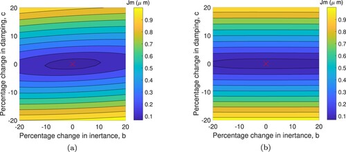
The default value for $J_m$ was 2.265 μm . Therefore, even in this worst case scenario, the performance is still improved over that default. These performance improvements as percentages are 52.8% and 53.6% for $G(s)$ and $Y(s)$ respectively.

This observation may not come as a surprise however. During the course of this study it has been found at every stage that the $J_m$ constraint is a key one. The trade-off performance between $J_1$ and $J_m$, and also $J_3$ and $J_m$ was discussed earlier. That discussion indicated that, for a relatively small degradation in $J_m$, a comparatively large improvement in $J_1$ or $J_3$ might be expected. As a result, the system is very sensitive to the value of $J_m$, and a small change in the system parameters can change the value of $J_m$ by a large amount. Hence, it is logical that varying the parameter values for each bush by $\pm 20\mathrm{\%}$ in this sensitivity study, that there would be large variation in the associated value for $J_m$. This analysis also shows that the bush $G(s)$ is more sensitive than $Y(s)$. Therefore, extra care would need to be taken when manufacturing $G(s)$ compared to $Y(s)$.

6. Discussions and conclusions

This study has explored the validity of incorporating inerters into an in-wheel motor system. Inerters were first incorporated into the bushes to try to control the magnetic gap deformation (termed $J_m$ here), without compromising body vertical acceleration (termed $J_1$ here), or the tyre dynamic load (termed $J_3$). This step was successful, and managed to reduce $J_m$ by 98.1%, thereby improving the motor reliability and longevity. The next step was to see if optimising the strut was able to improve any further on this 98.1% reduction. It was found that the improvement increased to 98.6% with all parameters optimised in a single pass. This relatively small increase could be explained by the position of the bushes relative to the motor when compared to the strut position. The bushes directly surround the rotor and stator, and hence have a large impact on the force imparted on the motor, whilst the strut does not. Hence the strut is not able to reduce $J_m$ by any further significant margin. It is this 98.6% improvement possible in the performance of $J_m$ which is the most significant finding of this study. This is due to the increase in reliability and longevity of the motor, without degrading the ride comfort or tyre grip over the default performance.

Inerters were then incorporated into the suspension strut to control $J_1$ and $J_3$. The performance improvement was initially found to be limited. However, this was then traced to the constraint applied on $J_m$. Initially, this constraint was simply relaxed and the resulting performance benefits for $J_1$ and $J_3$ were found. These benefits were considered impressive on initial inspection. However, the issues with relaxing this constraint are numerous. These issues include potentially worsening the reliability of the motor, as well as encouraging an unbalanced radial magnetic force to grow. This unbalanced radial magnetic force would have destructive properties for the overall system performance, and would also reduce the validity of the linear assumption made in this study. However, it did prove that the $J_m$ performance is critical to the overall performance of the system. The solution to this limited $J_1$ and $J_3$ improvement was to use the knowledge gained from the section surrounding improvements to $J_m$, and to include inerter-based absorbers in the bushes. Then all of the parameters could be optimised for $J_1$ and $J_3$ in a single pass. This gave performance improvements of 20.2% and 9.18% over the default values, without compromising the value of $J_m$.

This work has shown that the ride comfort of a vehicle with an in-wheel motor, as well as the road-holding, can be improved by using inerter-based absorbers. At the same time, it was shown that the motor longevity and reliability can be improved by reducing the magnetic gap deformation between rotor and stator, again by using inerter-based absorbers. It was shown with a sensitivity study, which varied the damping and inertance values by 20% from the optimum, that the resulting performance still improved over the default system. Therefore, it is highly beneficial to include inerter-based absorbers in an in-wheel motor system.

Disclosure statement

No potential conflict of interest was reported by the author(s).

Correction Statement

This article has been corrected with minor changes. These changes do not impact the academic content of the article.

Additional information

Funding

The authors gratefully acknowledge the support of the EPSRC: J.Z.J is supported by the Engineering and Physical Sciences Research Council (EPSRC) fellowship [grant number EP/T016485/1]. S.A.N. is supported by the Engineering and Physical Sciences Research Council (EPSRC) programme [grant number EP/R006768/1]. N.J.W. is supported by the EPSRC PhD scholarship. The authors also are grateful for the technical and financial support of Tenneco Automotive.

Notes

1 Both $J_1$ and $J_3$ are the conventional way of referring to these metrics, after they were proposed in [22], hence this study also uses that notation.

Appendix A.

Structure-immittance method

In this study only the three element layouts are considered. Hence, only the generic networks for the single inerter and single damper case are considered. To use these generic networks, the complexity can be reduced through ‘neglecting’ up to five of the six springs in either generic network. This is either achieved by setting k = 0 or $1/k=0$. Setting k = 0 is equivalent to removing a branch of the network. Whilst setting $1/k=0$ makes the spring infinitely stiff, and approximates a rigid connection.

These generic networks are used in combination with their associated equations, also from [28]. These are as follows: (A1) $\begin{array}{rl}{Y}_1(s)& =\frac{\mathrm{bc}{s}^3+b(k_4+k_6)s+c(k_2+k_6)}{\mathrm{bc}(\frac{1}{k_3})s^3+b{s}^2+\mathrm{cs}+k_2+k_4}\end{array}$(A1) (A2) $\begin{array}{rl}{Y}_2(s)& =\frac{\mathrm{bc}(\frac{1}{k_1}+\frac{1}{k_2})s^3+b{s}^2+\mathrm{cs}+k_3}{\mathrm{bc}(\frac{1}{k_1}+\frac{1}{k_5})s^3+c(\frac{1}{k_2}+\frac{1}{k_5})s^2+s}\end{array}$(A2) where $b⩾0$ and $c⩾0$ in each case. In addition to this, in Equation  (A1(A1) $\begin{array}{rl}{Y}_1(s)& =\frac{\mathrm{bc}{s}^3+b(k_4+k_6)s+c(k_2+k_6)}{\mathrm{bc}(\frac{1}{k_3})s^3+b{s}^2+\mathrm{cs}+k_2+k_4}\end{array}$(A1) ) at least three out of the parameters $k_2$, $1/k_3$, $k_4$ and $k_6$ must be set to zero. Similarly, in Equation  (A2(A2) $\begin{array}{rl}{Y}_2(s)& =\frac{\mathrm{bc}(\frac{1}{k_1}+\frac{1}{k_2})s^3+b{s}^2+\mathrm{cs}+k_3}{\mathrm{bc}(\frac{1}{k_1}+\frac{1}{k_5})s^3+c(\frac{1}{k_2}+\frac{1}{k_5})s^2+s}\end{array}$(A2) ) at least three out of the parameters $1/k_1$, $1/k_2$, $k_3$ and $1/k_5$ must be set to zero.

To demonstrate this method, the admittance function for layout III-2 will be derived. For this, the first generic absorber layout (Equation  (A1(A1) $\begin{array}{rl}{Y}_1(s)& =\frac{\mathrm{bc}{s}^3+b(k_4+k_6)s+c(k_2+k_6)}{\mathrm{bc}(\frac{1}{k_3})s^3+b{s}^2+\mathrm{cs}+k_2+k_4}\end{array}$(A1) )) is used. Then $1/k_2$, $1/k_4$, $k_6$, $k_8$ and $1/k_9$ must be set to zero. That leaves the admittance function thus: (A3) $Y(s)=\frac{1}{\frac{1}{c}+\frac{1}{\mathrm{bs}}}+\frac{k}{s}=\frac{\mathrm{cb}{s}^2+\mathrm{kbs}+\mathrm{ck}}{b{s}^2+\mathrm{cs}}$(A3) If a similar method is followed, all eight admittance functions can be found for the absorber layouts.

These admittance functions give a force-velocity relationship for the absorber layouts. As a result, they can simply replace a normal damping coefficient in an equation of motion in the Laplace domain. This is because the damper provides a force which corresponds to the relative velocity between its end points. The damper can be described as having an admittance function $Y(s)=c$ in this case.

Appendix B.

Derivation of ${\mathrm{J}}_{\mathrm{m}}$

For the performance equations in Section 2.3, the road input is defined using the same method as [22]. Hence it is defined as a time-varying displacement $x_0(t)$ for the tyre contact patch, derived from traversing a rigid road profile ($x_0^{\prime }(z)$, where z is the direction of travel) at a speed V. This leads to the relationship $x_0(t)=x_0^{\prime }(\mathrm{Vt})$. The spectral densities corresponding to this are then defined as follows: (A4) $S^{x_0}(f)=\frac{1}{V}{S}^{x_0^{\prime }}(n)$(A4) where f is frequency in Hz (cycles per second), n is the wave number in cycles per metre and f = nV. Consider an output variable $z(t)$ which is related to the input $x(t)$ by a transfer function $H(s)$, then the expectation of $z^2(t)$ can be defined as: (A5) $E[z^2(t)]={\int }_{-\mathrm{\infty }}^{\mathrm{\infty }}{|H(j2\mathrm{\pi f})|}^2{S}^{x_0}(f)\mathrm{d}f=\frac{1}{2\mathrm{\pi V}}{\int }_{-\mathrm{\infty }}^{\mathrm{\infty }}{|H(\mathrm{j\omega })|}^2{S}^{x_0^{\prime }}(n(\omega ))\mathrm{d}\omega$(A5) which follows the form of the accepted ${\mathcal{H}}_2$ norm. This permits $J_1$ and $J_3$ to be defined as discussed earlier in Equations  (4(4) $\begin{array}{rl}{J}_1& =2\pi (\mathrm{V\kappa }{)}^{\frac{1}{2}}{\left|\left|s{T}_{{\hat{x}}_0\to {\hat{x}}_2}\right|\right|}_2\end{array}$(4) ) and (5(5) $\begin{array}{rl}{J}_3& =2\pi (\mathrm{V\kappa }{)}^{\frac{1}{2}}{\left|\left|\frac{1}{s}{T}_{{\hat{x}}_0\to k_1({\hat{x}}_1-{\hat{x}}_0)}\right|\right|}_2\end{array}$(5) ) when combined with the road profile spectrum as suggested in [38]: (A6) $S^{x_0^{\prime }}(n)=\kappa {\left|n\right|}^{-2}$(A6) where κ has units of m${}^3$cycle${}^{-1}$.

MGD is defined as the relative displacement between the rotor and stator of the IWM, i.e. the relative displacement between $m_{32}$ and $m_{33}$ respectively in this model. This therefore follows the same relationship as the definition of $J_3$. This is because $J_3$ is defined as the force resulting from the relative deflection of the tyre, (i.e.: the stiffness of the tyre multiplied by the difference in displacement of the tyre and road). For $J_m$, the relative displacement, rather than a force, is required. Therefore the transfer function which relates the deflection of the rotor and stator, normalised by the road input, can be found. Namely: (A7) $T_{{\hat{x}}_0\to ({\hat{x}}_{33}-{\hat{x}}_{32})}$(A7) which will not be shown in this paper for simplicity. As with $J_3$, this must be a displacement, and hence the integrator ($\frac{1}{s}$) term is required.

Unlike the common $J_1$ and $J_3$ metrics however, $J_m$ does not use a standard ${\mathcal{H}}_2$ norm. The reason for this is because $J_m$ is frequency limited between 0 and 25 Hz (which correspond to 0 and 50π rad/s). A sum approximation to the integral is adopted for speed in MATLAB optimisations, with a frequency spacing of 0.1 rad/s providing sufficient accuracy without extensively increasing computation time. $J_m$ is described as follows: (A8) $J_m={(2\mathrm{\pi V\kappa }(\mathrm{\Delta \omega })\sum _{{\omega }_1}^{{\omega }_2}{\left|\frac{1}{s}{T}_{{\hat{x}}_0\to ({\hat{x}}_{33}-{\hat{x}}_{32})}\right|}^2)}^{\frac{1}{2}}$(A8) where all terms are as previously defined. This uses the same ‘square root of the sum of the square of the magnitudes’ approach as the ${\mathcal{H}}_2$ norm. However, it requires normalising. This is achieved by multiplying by the frequency step, $\mathrm{\Delta }\omega$. It is also worth noting that it does not have the same $\frac{1}{2\pi }$ term as in the ${\mathcal{H}}_2$ norm. As a result $2\mathrm{\pi V\kappa }$ needs to also be square rooted, rather than just the $\mathrm{V\kappa }$ of the $J_1$ and $J_3$ equations defined in [22].

In order to test the accuracy of the proposed $J_m$ metric, a version using the ${\mathcal{H}}_2$ norm was also suggested. This can be seen as follows: (A9) $J_{m,{\mathcal{H}}_2}=2\pi (\mathrm{V\kappa }{)}^{\frac{1}{2}}{\left|\left|\frac{1}{s}{T}_{{\hat{x}}_0\to ({\hat{x}}_{33}-{\hat{x}}_{32})}\right|\right|}_2$(A9) with all terms as previously defined in Section 2. As previously explained, this would include high frequency effects which would not be accurately represented as a result of the simple tyre model, and so this metric could not be used for optimisation. However, it could be used to test the accuracy of the $J_m$ metric. Setting ${\omega }_1$ as -40,000π rad/s (-20 kHz) and ${\omega }_2$ as 40,000π rad/s (20 kHz), with $\mathrm{\Delta }\omega$ being 0.001 rad/s, the output from Equations  (A8(A8) $J_m={(2\mathrm{\pi V\kappa }(\mathrm{\Delta \omega })\sum _{{\omega }_1}^{{\omega }_2}{\left|\frac{1}{s}{T}_{{\hat{x}}_0\to ({\hat{x}}_{33}-{\hat{x}}_{32})}\right|}^2)}^{\frac{1}{2}}$(A8) ) to (A9(A9) $J_{m,{\mathcal{H}}_2}=2\pi (\mathrm{V\kappa }{)}^{\frac{1}{2}}{\left|\left|\frac{1}{s}{T}_{{\hat{x}}_0\to ({\hat{x}}_{33}-{\hat{x}}_{32})}\right|\right|}_2$(A9) ) agreed to within the required degree of accuracy in this study (four significant figures). The reported value was different to the constraint value shown in Section 2.3 due to the high frequency effects, and so will not be shown here.

References

- Wu B, Offer GJ. Environmental impact of hybrid and electric vehicles.In: Environmental impacts of road vehicles: Past, present and future. 1st Edition. London: Royal Society of Chemistry; 2017. p. 133–156.
- Adams W. Electric motor; U.S. Patent US300827A. 24 June 1884.
- Murata S. Innovation by in-wheel-motor drive unit. Veh Syst Dyn. 2012;50(6):807–830. doi: 10.1080/00423114.2012.666354
- Liu M, Gu F, Huang J, et al. Integration design and optimization control of a dynamic vibration absorber for electric wheels with in-wheel motor. Energies. 2017;10(12):2069.
- Hrovat D. Influence of unsprung weight on ride quality. J Sound Vib. 1988;124:497–516. doi: 10.1016/S0022-460X(88)81391-9
- Campbell C. Automobile suspensions. 1st ed. London: Chapman and Hall; 1981.
- Esmailzadeh E, Vossoughi G, Goodarzi A. Dynamic modeling and analysis of a four motorized wheels electric vehicle. Veh Syst Dyn. 2001;35(3):163–194. doi: 10.1076/vesd.35.3.163.2047
- Tan D, Wu Y, Feng J, et al. Lightweight design of the in-wheel motor considering the coupled electromagnetic-thermal effect. Mech Based Des Struct Mach. 2022;50(3):935–953.
- Luo Y, Tan D. Study on the dynamics of the in-wheel motor system. IEEE Trans Veh Technol. 2012;61:3510–3518. doi: 10.1109/TVT.2012.2207414
- Wang Q, Li R, Zhu Y, et al. Integration design and parameter optimization for a novel in-wheel motor with dynamic vibration absorbers. J Braz Soc Mech Sci Eng. 2020;42:459. doi: 10.1007/s40430-020-02543-8
- Nagaya G, Wakao Y, Abe A. Development of an in-wheel drive with advanced dynamic-damper mechanism. JSAE Rev. 2003;24(4):477–481. doi: 10.1016/S0389-4304(03)00077-8
- Qin Y, He C, Shao X, et al. Vibration mitigation for in-wheel switched reluctance motor driven electric vehicle with dynamic vibration absorbing structures. J Sound Vib. 2018;419(1):249–267. doi: 10.1016/j.jsv.2018.01.010
- Wu H, Zheng L, Li Y. Coupling effects in hub motor and optimization for active suspension system to improve the vehicle and the motor performance. J Sound Vib. 2020;482(1):1–18.
- Liu M, Zhang Y, Huang J, et al. Optimization control for dynamic vibration absorbers and active suspensions of in-wheel-motor-driven electric vehicles. P I MECH ENG D-J AUT. 2020;234(9):2377–2392. doi: 10.1177/0954407020908667
- Li Z, Zheng L, Ren Y, et al. Multi-objective optimization of active suspension system in electric vehicle with in-wheel-motor against the negative electromechanical coupling effects. Mech Syst Signal Process. 2019;116:545–565. doi: 10.1016/j.ymssp.2018.07.001
- Long G, Ding F, Zhang N, et al. Regenerative active suspension system with residual energy for in-wheel motor driven electric vehicle. Appl Energy. 2020;260:114180. doi: 10.1016/j.apenergy.2019.114180
- Wang Y, Li P, Ren G. Electric vehicles with in-wheel switched reluctance motors: coupling effects between road excitation and the unbalanced radial force. J Sound Vib. 2016;372:69–81. doi: 10.1016/j.jsv.2016.02.040
- Smith MC. Synthesis of mechanical networks: the inerter. IEEE Trans Automat Contr. 2002;47:1648–1662. doi: 10.1109/TAC.2002.803532
- Wang FC, Su WJ. Impact of inerter nonlinearities on vehicle suspension control. Veh Syst Dyn. 2008;46(7):575–595. doi: 10.1080/00423110701519031
- Liu X, Jiang JZ, Titurus B, et al. Model identification methodology for fluid-based inerters. Mech Syst Signal Process. 2018;106:479–494. doi: 10.1016/j.ymssp.2018.01.018
- Swift SJ, Smith MC, Glover AR, et al. Design and modelling of a fluid inerter. Int J Control. 2013;86(11):2035–2051. doi: 10.1080/00207179.2013.842263
- Smith MC, Wang FC. Performance benefits in passive vehicle suspensions employing inerters. Veh Syst Dyn. 2004;42:235–257. doi: 10.1080/00423110412331289871
- Lazar I, Neild S, Wagg D. Vibration suppression of cables using tuned inerter dampers. Eng Struct. 2016;122:62–71. doi: 10.1016/j.engstruct.2016.04.017
- Luo J, Macdonald JH, Jiang JZ. Use of inerter-based vibration absorbers for suppressing multiple cable modes. Procedia Eng. 2017;199:1695–1700. doi: 10.1016/j.proeng.2017.09.370
- Lewis TD, Jiang JZ, Neild SA, et al. Using an inerter-based suspension to improve both passenger comfort and track wear in railway vehicles. Veh Syst Dyn. 2020;58(3):472–493. doi: 10.1080/00423114.2019.1589535
- Lewis TD, Li Y, Tucker GJ, et al. Improving the track friendliness of a four-axle railway vehicle using an inertance-integrated lateral primary suspension. Veh Syst Dyn. 2021;59(1):115–134. doi: 10.1080/00423114.2019.1664752
- Jiang JZ, Matamoros-Sanchez AZ, Goodall RM, et al. Passive suspensions incorporating inerters for railway vehicles. Veh Syst Dyn. 2012;50(sup1):263–276. doi: 10.1080/00423114.2012.665166
- Zhang SY, Jiang JZ, Neild SA. Passive vibration control: a structure–immittance approach. Proc R Soc A. 2017;473(2201):20170011. doi: 10.1098/rspa.2017.0011
- Zhang SY, Zhu M, Li Y, et al. Ride comfort enhancement for passenger vehicles using the structure-immittance approach. Veh Syst Dyn. 2021;59(4):504–525. doi: 10.1080/00423114.2019.1694158
- Guiggiani M. The science of vehicle dynamics: handling, braking, and ride of road and race cars. 2nd ed. Cham: Springer; 2018.
- Smith MC, Swift SJ. Design of passive vehicle suspensions for maximal least damping ratio. Veh Syst Dyn. 2016;54(5):568–584. doi: 10.1080/00423114.2016.1145242
- Sharp RS, Crolla DA. Road vehicle suspension system design – a review. Veh Syst Dyn. 1987;16(3):167–192. doi: 10.1080/00423118708968877
- Gillespie TD. Fundamentals of vehicle dynamics. 1st ed. Warrendale, PA: Society of Automotive Engineers; 1992.
- Schiehlen W. White noise excitation of road vehicle structures. Sadhana. 2006;31(4):487–503. doi: 10.1007/BF02716788
- Bender EK. Optimum linear preview control with application to vehicle suspension. Trans ASME J Basic Eng. 1968;90(2):213–221. doi: 10.1115/1.3605082
- White FM. Fluid mechanics. 7th ed. New York: McGraw Hill; 2011.
- Wang FC, Hong MF, Lin TC. Designing and testing a hydraulic inerter. Proc Inst Mech Eng C J Mech Eng Sci. 2011;225(1):66–72. doi: 10.1243/09544062JMES2199
- Robson JD. Road surface description and vehicle response. Int J Veh Des. 1979;1(1):25–35.