Bootstrapped inference for variance parameters, measures of heterogeneity and random effects in multilevel logistic regression models

Abstract

We used Monte Carlo simulations to assess the performance of three bootstrap procedures for use with multilevel data (the parametric bootstrap, the residuals bootstrap, and the nonparametric bootstrap) for estimating the sampling variation of three measures of cluster variation and heterogeneity when using a multilevel logistic regression model: the variance of the distribution of the random effects, the variance partition coefficient (equivalent here to the intraclass correlation coefficient), and the median odds ratio. We also described a novel parametric bootstrap procedure to estimate the standard errors of the predicted cluster-specific random effects. Our results suggest that the parametric and residuals bootstrap should, in general, be used to estimate the sampling variation of key measures of cluster variation and heterogeneity. The performance of the novel parametric bootstrap procedure for estimating the standard errors of predicted cluster-specific random effects tended to exceed that of the model-based estimates.

KEYWORDS:

• Bootstrap
• hierarchical model
• Monte Carlo simulations
• multilevel model
• random-effects model
• variance

1. Introduction

Multilevel models (mixed-effects models, random-effects models and hierarchical models) are increasingly being used across a wide range of disciplines. These models allow for analysis of data that have a multilevel or hierarchical structure (e.g. patients nested within hospitals or students nested within schools). Longitudinal data are also clustered (e.g. repeated measures nested within subjects). A primary use of these models is to estimate the association between subject outcomes (e.g. death within 30 days of hospital admission) and characteristics of the subject (e.g. age, sex and socioeconomic status) or cluster (e.g. size and type of hospital or geographic location). These models allow for estimation of standard errors of estimated regression coefficients that account for the lack of independence induced by the clustering of subjects. They also allow one to quantify heterogeneity in mean subject outcomes across clusters and to predict cluster effects on subject outcomes.

Historically, the focus of many applied analysts when using multilevel logistic regression models was exclusively on the odds ratio, which is a measure of association. More recently, there has been a growing interest in additionally reporting and interpreting measures of cluster variation and heterogeneity. Three important measures of cluster variation and heterogeneity (hereafter referred to as cluster variation) are: (i) the variance of the cluster-specific random effects, henceforth referred to as the cluster variance; (ii) the variance partition coefficient (VPC) also often referred to as the intraclass correlation coefficient (ICC); (iii) the median odds ratio (MOR). The VPC denotes the proportion of variation in the outcome that is due to systematic between-cluster differences [1,2]. The MOR was first proposed by Larsen et al. [3] for quantifying the magnitude of the effect of clustering (i.e. the cluster variance) as an odds ratio when using a multilevel logistic regression model. If one were to repeatedly sample at random two subjects with the same covariate values from different clusters, then the MOR is the median odds ratio between the subject at higher risk of the outcome and the subject at the lower risk of the outcome (where differences in risk are entirely due to differing cluster-specific random-effect values). The use of measures of cluster variation was subsequently popularized by a series of editorials and articles in the epidemiological literature [4–11].

There is often interest in testing whether the cluster variance is statistically significantly different from zero (and whether the VPC is different from zero and the MOR different from unity). This can be tested using either a modified Wald test or a modified likelihood ratio test (where the modification relates to testing on the boundary of the feasible parameter space; the cluster variance must be positive), with the latter being preferable [12]. The American Statistical Association, however, has recently suggested that researchers not draw conclusions solely based on tests of statistical significance [13]. Accordingly, it is important to be able to construct confidence intervals for measures of cluster variation. Since the sampling distribution of the cluster variance is often non-symmetric, normal theory-based confidence intervals can have poor performance [2]. Furthermore, methods for constructing confidence intervals for the VPC and the MOR have not been adequately described. There is a need to explore robust methods to construct confidence intervals for these three measures of cluster variation.

Multilevel regression models are increasingly being used in provider profiling to compare patient outcomes across healthcare providers or to compare student performance across schools [14–17]. When used for these purposes, the predicted cluster-specific random effects permit the quantification of the degree to which subject outcomes at one cluster (e.g. a hospital or school) differ, on average, from those at an average cluster, holding all covariates constant. With provider profiling, it is therefore important to be able to estimate and communicate the uncertainty in the predicted cluster-specific random effects, as these predictions are often used to hold providers to account, to provide information to support patient choice and to aid other types of decision-making. Presenting a confidence interval for each predicted cluster-specific random effect permits identification of those clusters that have performance that differs significantly from that of an average cluster and is an effective way of communicating the general lack of precision with which such effects are often estimated in empirical applications.

The bootstrap is a commonly used statistical procedure for estimating uncertainty and variability in estimated statistics [18]. There is a small literature on the use of bootstrap methods with multilevel data [19–25]. There are two limitations to the existing literature. First, the focus is almost exclusively on the multilevel linear regression model for use with continuous outcomes. One exception is an article that used bootstrap methods to develop a score test for testing whether the variance component was different from zero in generalized linear mixed models [25] (while not the focus of the article, another article provides a brief appendix discussing bootstrap approaches for generalized linear mixed models [26]). In biomedical research, binary or dichotomous outcomes are common [27]. Second, the focus of most of these articles was primarily on estimating variability in estimated regression coefficients and not on measures of cluster variation or in the predicted cluster-specific random effects. In particular, there is no research into whether the use of the bootstrap can result in improved estimates of the standard errors and confidence intervals of predicted cluster-specific random effects.

The objective of the current paper is to examine the use of the bootstrap with the multilevel logistic regression model. We focus on the use of the bootstrap for (i) estimating the sampling variability of measures of cluster variation (the cluster variance, the VPC and the MOR) and of the predicted cluster-specific random effects; (ii) constructing confidence intervals for these quantities. The paper is structured as follows: In Section 2, we first describe the parametric, residuals and nonparametric bootstrap procedures for use with multilevel data. We then propose a modified parametric bootstrap for making inferences about predicted cluster-specific random effects. In Section 3, we describe a series of Monte Carlo simulations designed to evaluate the performance of these procedures. In Section 4, we report the results of these simulations. In Section 5, we present a case study illustrating the application of these procedures to examine variation in patient mortality after hospitalization for acute myocardial infarction. Finally, in Section 6, we summarize our findings, place them in the context of the literature and make recommendations to researchers seeking to apply the multilevel bootstrap in their own work.

2. The multilevel bootstrap for multilevel logistic regression models

We assume that the reader is familiar with multilevel logistic regression [28] and the standard or conventional bootstrap [18]. Carpenter et al., van der Leeden et al. and Goldstein describe the use of the bootstrap with multilevel linear regression models [20–22,24]. We make appropriate modifications to two of the described procedures so as to be applicable to the multilevel logistic regression model. We also describe a new parametric bootstrap procedure to make inferences about the predicted cluster-specific random effects.

Let $Y_{ij}$ be a binary outcome variable denoting the occurrence of an event ($Y_{ij}=1$) or its non-occurrence ($Y_{ij}=0$), for the ith subject in the jth cluster and let ${\mathbf{X}}_{ij}$ denote a vector of covariates for this subject. This vector may include both subject- and cluster-level covariates and any cross-level interactions. Let K denote the number of clusters. We assume that the following random-intercept logistic regression model has been fit: $\text{logit}(p_{ij}=Pr(Y_{ij}=1))={\alpha }_0+{\alpha }_{0j}+{\mathbf{X}}_{ij}\mathit{\beta }$, where the cluster-specific random effect ${\alpha }_{0j}$ is assumed to be normally distributed with zero mean and constant variance, ${\alpha }_{0j}\sim N(0,{\tau }^2)$. We use the term ‘cluster variance’ to refer to the variance of the cluster-specific random effects (${\tau }^2$). Thus, the cluster variance is estimated directly.

In the current study, we fit all models by maximum likelihood estimation (adaptative quadrature with 7 quadrature points) in the R software using the glmer function of the lme4 package.

Post-estimation we can calculate the VPC. We use the latent variable formulation of the VPC, in which $\text{VPC}=\frac{{\tau }^2}{{\tau }^2+{\pi }^2/3}$ [1,2]. The MOR is defined $\text{MOR}=exp(\sqrt{2{\hat{\tau }}^2}\times {\mathrm{\Phi }}^{-1}(0.75))$, where $\mathrm{\Phi }$ denotes the cumulative distribution function of the standard normal distribution [3,9,28].

Post-estimation, we assign values to the cluster-specific random effects via empirical Bayes prediction. An important feature of empirical Bayes prediction is that the predicted values are shrunk towards the overall average as an increasing function of their unreliability. Essentially, the predicted values for small clusters are shrunk more than those for large clusters, reflecting the greater role of chance variability in determining the average outcomes observed in small clusters. The variance of these empirical Bayes predictions is therefore smaller than the estimated cluster variance for the population (${\tau }^2$). We will revisit this feature of empirical Bayes predictions when describing one of the bootstrap procedures.

We describe three different bootstrap procedures for use with multilevel logistic regression models: (i) the parametric bootstrap; (ii) the residuals bootstrap and (iii) the non-parametric bootstrap. In each case, the reported parameter estimates and model predictions are those obtained from fitting the above model to the original data. However, the standard errors and 95% confidence intervals are obtained from the bootstrap procedures. After describing the three bootstrap procedures, we describe why they cannot be used to make inferences about predicted cluster-specific random effects and so we describe a new parametric bootstrap procedure for this purpose.

2.1. The parametric bootstrap

For each of the K clusters, a new simulated cluster-specific random effect is drawn from the estimated parametric distribution of the cluster-specific random effects: ${\alpha }_{0j}^{\text{bs}}\sim N(0,{\hat{\tau }}^2),j=1,\dots ,K$. For each subject in each cluster, a new value for the linear predictor is computed using this simulated cluster-specific random effect, the estimated average intercept and the estimated vector of regression coefficients: $\text{logit}(p_{ij}^{\text{bs}})={\hat{\alpha }}_0+{\alpha }_{0j}^{\text{bs}}+{\mathbf{X}}_{ij}\hat{\mathit{\beta }}$. A new binary outcome is then simulated for each subject from a Bernoulli distribution: $Y_{ij}^{\text{bs}}\sim \text{Be}(p_{ij}^{\text{bs}})$. A random effects logistic regression is then fit to the new data consisting of ($Y_{ij}^{\text{bs}},{\mathbf{X}}_{ij}$). These data consist of the observed covariates and the new simulated binary outcome. The quantities of interest (e.g. the cluster variance, the VPC, the MOR or the predicted random effects) are then calculated in the usual way. This process is repeated B times. The empirical standard deviation of the quantity of interest is determined across the B bootstrap replicates. This is an estimate the standard error of the quantity of interest.

2.2. The residuals bootstrap

The parametric bootstrap described in the previous section assumed the random effects to be normally distributed with zero mean and constant variance. The residuals bootstrap relaxes this parametric assumption. The residuals bootstrap begins with the set of K predicted cluster-specific random effects obtained from fitting the model to the original data: $\{{\hat{\alpha }}_{0j}:j=1,\dots ,\text{K} }$. The predicted cluster-specific random effects are then centred around their sample mean (this is achieved by subtracting the average of the cluster-specific random effects from each cluster-specific random effect). Recall that the predicted random effects exhibit shrinkage. We therefore ‘reflate’ the predicted random effects so that their empirical variance is equal to the estimated cluster variance derived from the fitted model [21,22]. We do this by multiplying the predicted random effects by the square root of the ratio of the estimated cluster variance to the empirical variance of the K predicted random effects. For each of the K clusters, a new cluster-specific random effect is drawn with replacement from this modified set of predicted cluster-specific random effects. The process then proceeds identically as in the parametric bootstrap.

2.3. The nonparametric bootstrap

Goldstein described a nonparametric bootstrap in which a bootstrap sample of clusters is selected from the original data [22]. Once a cluster has been selected, all of the subjects in that cluster are included in the bootstrap analytic sample. Clusters are drawn with replacement. When a cluster is drawn multiple times in a given bootstrap sample, these replicate clusters are given different cluster identifiers to distinguish them in the fitted model. Once a bootstrap sample has been selected, the procedure proceeds in an identical fashion to the two previous procedures. While van der Leeden et al. refer to this procedure as the cases bootstrap [20], we use the terminology of Goldstein [22] and refer to it as the nonparametric bootstrap.

Davison and Hinkley describe two different versions of the nonparametric bootstrap for multilevel data [19]. The first version, which is identical to that described above, draws a bootstrap sample of clusters and then selects all of the subjects contained in those clusters. The second version draws a bootstrap sample of clusters and then selects a bootstrap sample of the subjects contained in those clusters. They suggest that the former approach is preferable to the latter procedure, as it ‘more closely mimics the variation properties of the data’ (p. 101). Goldstein similarly favours the former approach when describing a nonparametric multilevel bootstrap [22]. Thus, we do not consider the latter approach further in this article.

There are a few differences between the nonparametric bootstrap and the parametric or residuals bootstrap that merit highlighting. An advantage to the parametric and residuals bootstrap procedures is that each bootstrap sample will be of the same size as the original sample. However, with the nonparametric bootstrap, the size of the bootstrap samples will vary somewhat across bootstrap replicates, especially when there are few clusters and these clusters vary in size. However, Goldstein suggests that for moderate or large sample sizes, the effect of this variability will be minimal. A second difference is that both the parametric and residuals bootstrap assume that the covariates are fixed. Thus, in each bootstrap sample, the distribution of baseline covariates is identical to that in the original sample. Only the binary outcomes may differ from what was observed in the original sample. However, with the nonparametric bootstrap procedure, the distribution of baseline covariates may vary across bootstrap samples. The former approaches may therefore be conceptually more appealing in a designed experiment in which the distribution of covariates is under the control of the investigator. The latter may be conceptually more appealing in observational studies comparing variation in outcomes for patients hospitalized with a given medical condition or for students in schools. These are both settings in which one can think of the observed sample as a random sample from a larger population of clusters in which there is inherent variability in cluster size (i.e. the patients in a given hospital can be viewed as one possible realization of the patients who could have been treated at the given hospital).

2.4. A parametric bootstrap procedure for inferences about predicted cluster-specific random effects

The three bootstrap procedures described above can be used to make inferences about estimated model parameters (e.g. the regression coefficients and the cluster variance) and quantities derived directly from these parameters (e.g. VPC and MOR). However, these bootstrap procedures cannot be used to make inferences about the predicted cluster-specific random effects. When using the parametric bootstrap, one draws a new cluster-specific random effect from the estimated normal distribution with mean zero and whose variance is equal to the cluster variance. Thus, for a given cluster in the original data, the mean of the B simulated cluster-specific random effects will be zero and will not be an estimator for the original predicted cluster-specific random effect. A similar problem would occur with the residuals bootstrap. With the nonparametric bootstrap another problem arises. Since one selects a random sample of clusters, in a given bootstrap sample, some clusters will be represented multiple times while others will not be selected at all. Thus, in the bootstrap sample, there is no longer a correspondence between the sampled clusters and the original clusters.

We describe a modified parametric bootstrap for making inferences about predicted cluster-specific random effects (alternatively, for estimating the posterior mean of the random effects conditional on the observed data). From the fitted model, we obtain ${\hat{\alpha }}_{0j}$ and $\text{se(}{\hat{\alpha }}_{0j})$, which denote the predicted random effect and its estimated standard error for the jth cluster (the standard error was obtained from the model-based estimation procedure). Then for each cluster, in the kth bootstrap replicate, we simulate a cluster-specific random effect: ${\alpha }_{0j}^{\text{bs(k)}}\sim \text{N}({\hat{\alpha }}_{0j},\text{se}({\hat{\alpha }}_{0j}{)}^2)$. Having simulated a cluster-specific random effect from this cluster-specific normal distribution, we then inflate these simulated cluster-specific random effects so that their sample variance is equal to the cluster variance obtained from the model fitted to the original sample. This inflation process is identical to how the predicted cluster-specific random effects were inflated when using the residuals bootstrap. Once the inflated simulated cluster-specific random effects have been obtained, the procedure then proceeds in a fashion identical to the parametric and residuals bootstrap.

2.5. Bootstrap confidence intervals

While there are large number of procedures for constructing bootstrap confidence intervals [18,19], we limit our discussion to two popular approaches: normal-theory-based confidence intervals and bootstrap percentile intervals.

The normal-theory approach uses the standard deviation of the statistic or quantity of interest across the B bootstrap samples as the bootstrap estimate of the standard error of the statistic or quantity of interest. The corresponding 95% normal theory bootstrap confidence interval is then $\hat{\beta }\pm 1.96\text{s}{\text{e}}_{\text{BS}}(\hat{\beta })$, where $\hat{\beta }$ denotes the estimated statistic or quantity of interest from the original sample, while $\text{s}{\text{e}}_{\text{BS}}(\hat{\beta })$ denotes the bootstrap estimate of the standard error of the statistic or quantity of interest (i.e. the standard deviation of the statistic or quantity of interest across the B bootstrap samples).

Bootstrap percentile intervals are based on the empirical distribution of the statistic or quantity of interest across the B bootstrap samples. The upper and lower limits of a 95% bootstrap percentile interval for the statistic of interest are the 2.5th and 97.5th percentiles of this empirical distribution.

The first approach requires the assumption that the sampling distribution of the statistic of interest is normal, while the second approach does not make any parametric assumptions. However, the first approach may require substantially fewer bootstrap replicates (B) than the second approach. It has been suggested that standard deviations can be estimated with relatively few bootstrap replicates (B ≤ 200), while estimating of percentiles requires substantially more bootstrap replicates (B ≥ 1000) [18] (future research may be required to examine whether these guidelines are applicable to the multilevel bootstrap). We would not recommend the normal theory approach for constructing confidence intervals for the cluster variance, the VPC and the MOR as their sampling distributions are likely to be skewed and therefore non-normal.

3. Monte Carlo simulations – design

We designed a series of Monte Carlo simulations to compare the performance of the three bootstrap procedures described in Section 2 to estimate the sampling variability of the multilevel logistic regression model parameters and associated statistics. We also examined the performance of the modified parametric bootstrap for making inferences about the predicted cluster-specific random effects. Our focus is on the random-intercept logistic regression model. Earlier studies focused on the use of the bootstrap to estimate the sampling variability of the regression coefficients and cluster variance in the multilevel linear model. In contrast, our primary focus is on estimating the sampling variance of four different quantities of interest in the multilevel logistic regression model: (i) the cluster variance (${\tau }^2$); (ii) the VPC; (iii) the MOR and (iv) the cluster-specific random effects (${\alpha }_{0j}$). Our focus is on these four quantities as they are of key importance when studying variation in outcomes across clusters. We used one set of simulations to examine the use of the bootstrap to make inferences about the first three quantities and a second set of simulations to examine inferences about the fourth quantity. For completeness, we also evaluate the performance of bootstrap procedures for making inferences about the regression coefficients.

3.1. Data generating process

We simulated data for N_subjects nested within each of N_cluster clusters (for a total sample size of N_subjects × N_cluster). For each of the N_cluster clusters, we simulated a cluster-specific random effect: ${\alpha }_{0j}\sim N(0,{\tau }^2)$. For each of the N_subjects × N_cluster subjects we simulated a baseline covariate from a standard normal distribution: $x_{ij}\sim N(0,1)$. For each subject, a linear predictor was computed as: $\text{L}{\text{P}}_{ij}={\alpha }_0+{\alpha }_{0j}+{\alpha }_1{x}_{ij}$, where ${\alpha }_0=-0.25$ and ${\alpha }_1=1$ (these denote the fixed effects in the model). A binary outcome was generated for each subject from a Bernoulli distribution with parameter $p_{ij}=exp(\text{L}{\text{P}}_{ij})/(exp(\text{L}{\text{P}}_{ij})+1)$.

3.2. Statistical analyses

In the simulated dataset, we fit a random-intercept logistic regression model using the adaptive Gauss-Hermite approximation to the log-likelihood with seven quadrature points. We extracted and calculated the following quantities from the fitted model: (i) the estimated cluster variance (${\hat{\tau }}^2$); (ii) the estimated VPC; (iii) the estimated MOR; (iv) the estimated fixed intercept (α₀) and its model-based standard error; (v) the estimated fixed slope (α₁) and its model-based standard error. We delay discussion of the predicted cluster random effects until Section 3.5, as these will require a separate set of Monte Carlo simulations.

We drew B = 2000 bootstrap samples from the simulated dataset. The statistical analyses described in the previous paragraph were conducted in each of the B bootstrap samples. Let ${\hat{\tau }}_{\text{bs}(k)}^2$denote the estimated cluster variance in the kth bootstrap sample. Let $\text{VP}{\text{C}}^{\text{bs}(k)}$and $\text{MO}{\text{R}}^{\text{bs}(k)}$denote the estimated VPC and MOR in the kth bootstrap sample, respectively. Let ${\alpha }_0^{\text{bs}(k)}$and ${\alpha }_1^{\text{bs}(k)}$ denote the estimated fixed intercept and fixed slope in the kth bootstrap sample, respectively. We computed the standard deviation of ${\hat{\tau }}_{\text{bs}(k)}^2$, $\text{VP}{\text{C}}^{\text{bs}(k)}$, $\text{MO}{\text{R}}^{\text{bs}(k)}$, ${\alpha }_0^{\text{bs}(k)}$, and ${\alpha }_1^{\text{bs}(k)}$across the B bootstrap samples. These are the bootstrap estimates of the standard deviation of the sampling distribution of the quantity of interest. This process was conducted three times, once for each of the three bootstrap procedures.

We constructed 95% confidence intervals for each of the quantities of interest. For the cluster variance, VPC, and the MOR, we constructed bootstrap percentile intervals using each of the three bootstrap procedures. For the two fixed effects we constructed model-based 95% confidence intervals using the estimated standard errors of the fixed effects obtained from the fitted model in the original simulated sample. Then, for each bootstrap procedure we constructed two bootstrap confidence intervals: (i) using normal-theory methods and the bootstrap estimate of the standard error of the fixed effects; (ii) using bootstrap percentile intervals.

3.3. Summarizing the results of the simulations

The procedure described in Section 3.1 (simulating the data) and Section 3.2 (applying the bootstrap to a simulated dataset) was repeated 200 times. Thus, we simulated 200 datasets and in each of these 200 datasets, we drew 2000 bootstrap samples using each of the three bootstrap procedures. This process was computationally intensive, as it involved fitting 1,200,200 multilevel logistic regression models for each scenario (200 in the main simulated datasets + (200 × 2,000 × 3) in the bootstrap samples).

The true variability of the sampling distribution of each of the quantities of interest (${\tau }^2$, VPC, MOR, α₀ and α₁) was determined by computing the standard deviation of the estimated quantities across the 200 simulated datasets. These standard deviations reflect the true sampling variability of the quantities of interest.

For each of these quantities of interest, we obtained a bootstrap estimate of the standard error of that quantity in each of the 200 simulated datasets (as described in Section 3.2). We computed the mean of the estimated bootstrap standard error across the 200 simulated datasets. We then computed the ratio of the mean estimated standard deviation of the sampling distribution to the true standard deviation of the sampling distribution of the quantity of interest. If this ratio is equal to one, then the bootstrap estimate of the sampling variability is accurately estimating the variation of the sampling distribution. If this ratio is greater than one, then the bootstrap estimate of the sampling variability is biased upwards (the bootstrapped standard errors are too large), and if it is less than one, the bootstrap estimate of the sampling variability is biased downwards (the bootstrapped standard errors are too small).

For each quantity and each confidence interval, we computed the proportion of estimated 95% confidence intervals that contained the true value of the quantity. Due to our use of 200 simulation replicates, an empirical coverage rate that was less than 0.920 or that was greater than 0.980 was judged to be statistically significantly different from the advertised rate of 0.95.

3.4. Factors in the design of the simulations

We used a full-factorial design in which the following three factors were allowed to vary: (i) the number of subjects per cluster (N_subjects); (ii) the number of clusters (N_clusters); (iii) the cluster variance (${\tau }^2$). The number of subjects per cluster took two values: 10 and 20. The number of clusters took three values: 25, 50 and 100. The cluster variance took four values: 0.033, 0.173, 0.366 and 0.822 (these correspond to VPCs of 0.01, 0.05, 0.10 and 0.20, respectively and to MORs of 1.19, 1.49, 1.78 and 2.37, respectively). We thus considered 24 different scenarios (which involved fitting a total of 28,804,800 multilevel logistic regression models). The simulations were conducted using the R statistical programming language (version 3.5.1).

3.5. Simulations to examine the performance of the modified parametric bootstrap for making inferences about predicted cluster-specific random effects

We conducted a set of simulations to compare the performance of the modified parametric bootstrap procedure to make inferences about the N_cluster predicted cluster-specific random effects and their standard errors (${\hat{\alpha }}_{0j}$ and $\text{se}({\hat{\alpha }}_{0j})$).

These simulations were similar to those described above, with one modification. This modification was due to the fact that the predicted cluster-specific random effects are not, in themselves, parameters. Thus, rather than generate a set of N_cluster random effects within each of the 200 replicates for a given scenario (as was done in the simulations described above), we generated N_cluster random effects that were then fixed across the 500 replicates for a given scenario (i.e. the cluster-specific random effects for a given cluster did not vary across simulation replicates). To do otherwise, and simulate the cluster-specific random effects within each iteration of the simulation, would result in the mean cluster-specific random effect for each observed cluster being zero across the simulation iterations. While this modification may appear atypical, such an approach has previously been used when examining the effect of misspecification of the distribution of the random effects when making inferences about cluster-specific random effects [29].

The multilevel logistic regression model fit in each of the 500 simulated datasets provided predicted values for the cluster-specific random effects and their associated standard errors (${\hat{\alpha }}_{0j}$ and $\text{se}({\hat{\alpha }}_{0j})$). We examined the degree to which the model-based standard errors ($\text{se}({\hat{\alpha }}_{0j})$) accurately estimated the standard deviation of the sampling distribution of the predicted random effects (${\alpha }_{0j}$). We did the following for each cluster: (i) computed the standard deviation of each predicted cluster random effect (${\hat{\alpha }}_{0j}$) across the 500 simulated datasets (i.e. the true sampling variability due to sampling different individuals in each dataset); (ii) computed the mean estimated model-based standard error ($\text{se}({\hat{\alpha }}_{0j})$) of each predicted cluster random effect across the 500 datasets (i.e. the model-based estimate of the sampling variability) and (iii) computed the ratio of the quantity obtained in (ii) to that obtained in (i). If this ratio is equal to one, then the estimated model-based standard error is accurately estimating the standard deviation of the sampling distribution of the predicted cluster random effect. If this ratio is greater than one, then the model-based estimate of the sampling variability is biased upwards (the model-based standard error is too large), and if it is less than one, the model-based estimate of the sampling variability is biased downwards (the model-based standard error is too large).

We then repeated this process using the modified parametric bootstrap estimate of the standard error of the predicted cluster-specific random effect. For a given simulation replicate, we had B = 2000 bootstrap replicates. We used the standard deviation of each predicted cluster random effect ${\alpha }_{0j}^{\text{bs}(k)}$(k = 1, … , 2000) as the bootstrap estimate of the standard error for each cluster.

Note that examining the sampling variability of the random effects was done separately for each of the N_cluster random effects. When conducting this procedure for the predicted cluster-specific random effects, we obtained N_cluster ratios, one for each of the predicted cluster-specific random effects. We summarized each distribution of N_cluster ratios using the minimum, 25th percentile, median, 75th percentile and the maximum.

Within each bootstrap replicate for each simulation replicate, we constructed confidence intervals for the predicted cluster-specific random effects and determined whether the estimated confidence intervals contained the true cluster-specific random effects that had been generated prior to any of the simulation replicates. For a given cluster, we computed the proportion of confidence intervals across all bootstrap and simulation replicates that contained the true value of the cluster-specific random effect. This was the empirical coverage rate of the bootstrap confidence interval. We thus obtained N_cluster empirical coverage rates, one for each of the N_cluster clusters. For each simulation replicate, we constructed three sets of 95% confidence intervals for each cluster-specific random effect: (i) normal-theory-based confidence intervals using the model-based standard errors for the predicted cluster-specific random effects; (ii) bootstrap confidence intervals using normal-theory methods and the bootstrap estimates of the standard errors of the predicted cluster-specific random effects and (iii) bootstrap percentile intervals.

We examined a total of 28 different scenarios. We examined the 24 scenarios considered above in the primary set of simulations. We also examined four additional scenarios in which the number of clusters and number of subjects per cluster were equal to 25 and 100, respectively, and the cluster variance was the same as the four values in the primary set of simulations. The rationale for this extra set of four scenarios was to examine the quality of inferences about cluster-specific performance in settings with low numbers of clusters, but large cluster sizes (i.e. hospitals).

For this second set of simulations we used 500 simulation replicates for each scenario and 2000 bootstrap samples per simulation replicate (we were able to use 500 simulation replicates as only one bootstrap procedure was being examined in this set of simulations). This second set of simulations was also computationally intensive, as it involved fitting 1,000,500 multilevel logistic regression models for one scenario (500 in the main simulated datasets + (500 × 2000) in the bootstrap samples). Across the 28 scenarios, this entailed fitting 28,014,000 multilevel logistic regression models (for a total of 56,818,800 multilevel logistic regression models across the two sets of simulations).

4. Monte Carlo simulations – results

4.1. Inferences on measures of variance and heterogeneity

The ratio of the mean bootstrap estimate of the standard error of the sampling distribution of the given quantity to the empirical standard deviation of the sampling distribution of the estimated quantity is reported in Figure 1 (cluster variance, τ²), Figure 2 (VPC) and Figure 3 (MOR). Each figure is a dot chart, with 24 horizontal lines, one for each of the 24 scenarios in the Monte Carlo simulations. The first scenario (reported on the top horizontal line of the dot chart), for example, is labelled ‘100 & 20 & 0.2’ to indicate that in this scenario there are 100 clusters, 20 subjects per cluster, and a VPC of 0.2 (corresponding to a cluster variance of 0.822). The other scenarios are labelled in a similar fashion. On each horizontal line are three plotting symbols, one depicting the estimated ratio for each of the three bootstrap procedures. On each figure, we have superimposed a vertical line denoting a ratio of one. When the ratio is equal to one, then the standard deviation of the bootstrap estimates accurately estimates the empirical standard deviation of the sampling distribution of the quantity of interest. When the ratio is less than one than the bootstrap standard error underestimates the true sampling variability and when the ratio is greater than one the bootstrap standard error overestimates the true sampling variability. Note that the same scale for the horizontal axis is used for all three figures.

Figure 1. Ratio of mean bootstrap estimate of standard deviation to the empirical standard deviation of sampling distribution: τ².

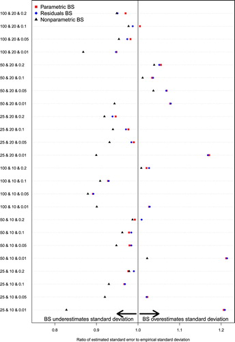
Figure 2. Ratio of mean bootstrap estimate of standard deviation to the empirical standard deviation of sampling distribution: VPC.

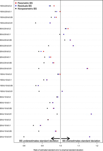
Figure 3. Ratio of mean bootstrap estimate of standard deviation to the empirical standard deviation of sampling distribution: MOR.

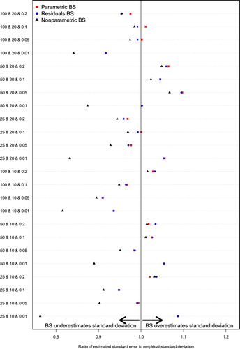
Figure 1 shows that when estimating the standard deviation of the sampling distribution of the cluster variance (τ²), the ratio of the mean bootstrap estimate of the standard deviation to the empirical standard deviation of the sampling distribution ranged from 0.89 to 1.21 for the parametric bootstrap (squares), with a median of 0.99 across the 24 scenarios. The standard deviation of the ratio across the 24 scenarios was 0.082. For the residuals bootstrap (circles), the corresponding range was 0.89–1.21, with a median of 0.99. The standard deviation of the ratio across the 24 scenarios was again 0.082. For the nonparametric bootstrap (triangles), the corresponding range was 0.83–1.04, with a median of 0.95. The standard deviation of the ratio across the 24 scenarios was 0.054.

For each bootstrap procedure, we used a linear model to regress the absolute deviation of the 24 ratios from unity on the three factors in the simulation (number of clusters, number of subjects per cluster and cluster variance). Each of these factors was treated as a categorical variable in the linear model. For the parametric bootstrap, only the cluster variance was associated with variation in the absolute deviation of the variance ratio from unity (p = .01). The number of clusters (p = .54) and number of subjects per cluster (p = .47) were not associated with variation in this deviation. The absolute deviation of the ratio from unity decreased by between 0.08 and 0.09 when the VPC was 0.05, 0.10 or 0.20 compared to when the VPC was equal to 0.01. Thus, the ratio was further from unity when the VPC was equal to 0.01 compared to larger values of VPC. Similar results were obtained when a linear model was used for the results of the simulations when the residuals bootstrap procedure was used. For the nonparametric bootstrap, both the number of clusters (p = .02) and the cluster variance (p = .02) were associated with the variation in the absolute deviation of the ratio from unity. When the number of clusters was equal to 50, the absolute deviation of the ratio from unity decreased by 0.05 compared to when the number of clusters was equal to 25. When the VPC was equal to 0.10 or 0.20, the absolute deviation of the ratio from unity decreased by 0.05 or 0.06 compared to when the VPC was equal to 0.01.

Figure 2 shows that when estimating the standard deviation of the sampling distribution of the VPC, the ratio of the mean bootstrap estimate of the standard deviation to the empirical standard deviation of the sampling distribution ranged from 0.88 to 1.17 for the parametric bootstrap, with a median of 0.98 across the 24 scenarios. The standard deviation of the ratio across the 24 scenarios was 0.079. For the residuals bootstrap, the corresponding range was 0.88–1.17, with a median of 0.97. The standard deviation of the ratio across the 24 scenarios was 0.081. For the nonparametric bootstrap, the corresponding range was 0.80–1.03, with a median of 0.93. The standard deviation of the ratio across the 24 scenarios was 0.057.

The general patterning of the ratios for the VPC in Figure 2 largely mimic those for the cluster variance shown in Figure 1. The similarity in the patterning of the ratios for the cluster variance and VPC is perhaps expected given that the latter is a deterministic function of the former, $\text{VPC}=\frac{{\tau }^2}{{\tau }^2+{\pi }^2/3}$.

Figure 3 shows that when estimating the standard deviation of the sampling distribution of the MOR, the ratio of the mean bootstrap estimate of the standard deviation to the empirical standard deviation of the sampling distribution ranged from 0.91 to 1.10 for the parametric bootstrap, with a median of 1.00 across the 24 scenarios. The standard deviation of the ratio across the 24 scenarios was 0.050. For the residuals bootstrap, the corresponding range was 0.91–1.10, with a median of 0.99. The standard deviation of the ratio across the 24 scenarios was 0.051. For the nonparametric bootstrap, the corresponding range was 0.76–1.07, with a median of 0.95. The standard deviation of the ratio across the 24 scenarios was 0.079.

The general patterning of the ratios for the MOR, shared many similarities with the above two sets of results; again this is perhaps expected given that the MOR is also a deterministic function of the cluster variance, $\text{MOR}=exp(\sqrt{2{\hat{\tau }}^2}\times {\mathrm{\Phi }}^{-1}(0.75))$.

In summarizing the first set of simulations, in general, the parametric and residuals bootstrap should be preferred over the nonparametric bootstrap. The median ratio for the former two bootstrap procedures was always closer to unity than was the ratio for the nonparametric bootstrap procedure.

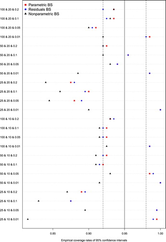
Empirical coverage rates of estimated 95% confidence intervals are reported in Figure 4. Note that since we use only bootstrap percentile interval for these quantities, and because the VPC and MOR are derived directly from the cluster variance, then empirical coverage rates for confidence intervals for these three quantities are identical. We have superimposed three vertical lines on this figure. The middle solid vertical line denotes the advertised coverage rate of 0.95. The outer two dashed vertical lines denote coverage rates of 0.92 and 0.98, such that empirical coverage rates between these two quantities are not statistically significantly different from the advertised rate (based on a standard normal -theory test). When the cluster variance was low (VPC = 0.01), the empirical coverage rate from the nonparametric bootstrap tended to diverge from those of the other two bootstrap procedures (which had coverage rates very similar to one another). When the number of clusters was low (K = 25), all three bootstrap procedures tended to result in confidence intervals with suboptimal coverage rates. In general, the nonparametric bootstrap resulted in confidence intervals with empirical coverage rates that were lower than those for the other two bootstrap procedures. Results were inconsistent as to which of the parametric and residuals bootstrap was to be preferred, with differences between the two often being negligible.

Figure 4. Empirical coverage rates of 95% confidence intervals for τ²/VPC/MOR.

4.2. Inferences for fixed effects

As inferences on fixed effects were of secondary interest, these results are reported in Appendix A in the online supplemental material.

4.3. Inferences on predicted cluster-specific random effects

The performance of the modified parametric bootstrap procedure for estimating the standard errors of predicted cluster-specific random effects is reported in Figure 5. We compared two procedures for estimating these standard errors: (i) model-based estimates of the standard errors of the predicted random effects derived from the fitted random effects logistic regression model and (ii) the modified parametric bootstrap. The results are presented using a dot chart with one row per scenario. On each row and for each of the two estimation procedures are five plotting symbols, representing the minimum (solid square), 25th percentile (solid circle), median (solid triangle), 75th percentile (upside down hollow triangle), and maximum (hollow square with diagonal cross) of the N_cluster ratios comparing the mean estimated standard error to the empirical standard deviation of the sampling distribution of the random effects across the N_cluster random effects (the results for each estimation procedure have been jittered vertically so as to not obscure each other).

Figure 5. Ratio of mean estimated standard error to empirical standard deviation of sampling distribution.

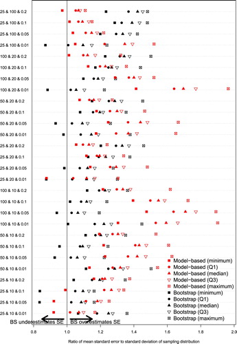
Across many of the 28 scenarios (recall that we added four new scenarios with 25 clusters and 100 subjects per cluster), the use of the modified parametric bootstrap tended to result in estimates of the standard errors of the predicted cluster-specific random effects that were closer to the standard deviation of the empirical sampling distribution than were the model-based estimates of standard errors. A notable exception was when K = 25 and there was N = 100 subjects per cluster and the VPC was at least 0.05.

Across the 28 scenarios, the median ratio of the mean model-based estimate of the standard error to the standard deviation of the empirical sampling distribution across the N_cluster random effects (solid triangles) ranged from 1.07 to 1.71, with a median of 1.30 (25th and 75th percentiles: 1.16 and 1.41). For the modified parametric bootstrap procedure, the range of ratios was 1.05–1.42, with a median of 1.20 (25th and 75th percentiles: 1.10 and 1.27). In general, the bootstrap procedures had superior performance to that of the model-based estimates of the standard errors of the cluster-specific random effects. These findings suggest that, on average, the modified parametric bootstrap results in improved estimates of the standard errors of the cluster-specific random effects compared to the model-based estimates.

In a given scenario, there are N_cluster cluster-specific random effects. Thus, there are N_cluster empirical coverage rates for a given scenario and for a given estimation procedure. Figure 6 depicts the median empirical coverage rate across the N_cluster random effects. Coverage of model-based confidence intervals, normal-theory parametric bootstrap confidence intervals, and parametric bootstrap percentile intervals are reported (unlike Figure 5, in which we report a five-number summary for each of the two estimation methods, the use of three methods for constructing confidence intervals resulted in a figure that was too cluttered and difficult to interpret if a five-number summary was used).

Figure 6. Coverage rates of 95% CIs for cluster-specific random effects.

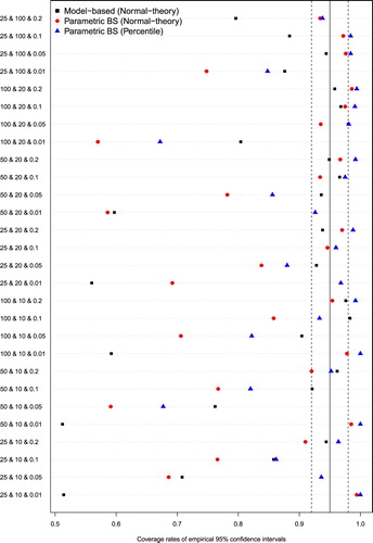
The median empirical coverage rates of the model-based confidence intervals across the N_cluster random effects ranged from 0.51 to 0.98, with a median of 0.92 (25th and 75th percentiles: 0.79 and 0.96). The median empirical coverage rates of the normal-theory bootstrap confidence intervals across the N_cluster random effects ranged from 0.57–0.99, with a median of 0.93 (25th and 75th percentiles: 0.76 and 0.97). The median empirical coverage rates of the bootstrap percentile intervals across the N_cluster random effects ranged from 0.67 to 1.00, with a median of 0.96 (25th and 75th percentiles: 0.88 and 0.99).

In general, coverage rates were poor for the model-based confidence intervals when the cluster variance was low (VPC = 0.01), and improved as the cluster variance increased. Except when either the number of subjects per cluster was equal to 100 or both the number of clusters and subjects per cluster were high (100 and 20, respectively), then the percentile bootstrap had superior coverage compared to the model-based confidence intervals when the cluster variance was low (VPC = 0.01). In all 28 scenarios, the median empirical coverage rate for the parametric bootstrap percentile intervals was higher than the median empirical coverage rate for the parametric bootstrap normal-theory confidence intervals.

5. Case study

The primary objective of the study was to evaluate the performance of difference bootstrap procedures for use with the multilevel logistic regression model. To illustrate the applications of these procedures using real data, a case study is described and reported in Appendix B in the online supplemental material.

6. Discussion

We examined the performance of three different bootstrap procedures for estimating the standard deviation of the sampling distribution of different estimated quantities in a random effects logistic regression model: the cluster variance the VPC, the MOR and the fixed effects. We also proposed a new parametric bootstrap procedure for estimating the standard errors and 95% confidence intervals of the predicted cluster-specific random effects. We summarize our findings and recommendations as follows: first, the parametric and residuals bootstrap resulted in more accurate estimation of the sampling variance of the cluster variance, the VPC and the MOR than did the nonparametric bootstrap. Second, the three bootstrap procedures had approximately equivalent performance for estimating standard errors of fixed effects. Third, the modified parametric bootstrap tended to result in improved estimates of the standard errors of predicted cluster-specific random effects when the number of clusters or number of subjects per cluster was not large.

Prior research on the multilevel bootstrap was restricted to settings with continuous outcomes [19,20,21,22]. In biomedical research, binary or dichotomous outcomes are common. We have described three bootstrap procedures for use with the multilevel logistic regression model. The use of these procedures allows for quantification of the uncertainty in measures of cluster variation in subject outcomes. Furthermore, none of these prior studies examined the use of bootstrap procedures for estimating the standard errors of predicted cluster-specific random effects. In provider profiling there is often an interest in creating confidence intervals around these quantities. The current paper describes a novel bootstrap procedure for this purpose.

When using the residuals bootstrap with the multilevel linear model, Carpenter et al. and Goldstein describe a procedure for reflating the set of predicted random effect values so that they have the correct variance [21,22]. We found that, in the context of the multilevel logistic regression model, the proposed inflation factor resulted in relatively good performance. The residuals bootstrap had poor performance when the inflation factor was omitted (results not shown).

Multilevel logistic regression models are increasingly used to quantify variation and heterogeneity in outcomes across clusters [28]. Measures such as the cluster variance, the VPC and the MOR allow for a quantification of variance and heterogeneity. We demonstrated that multilevel bootstrap procedures can be used to estimate the sampling variability of these quantities. There is often interest in testing whether the cluster variation is statistically significantly different from zero. This can be tested using either a modified Wald test or a modified likelihood ratio test, with the latter being preferable [12]. The use of the bootstrap can be used to complement these tests. The American Statistical Association has recently released a statement on the use and interpretation of p-values [13]. Among the many suggestions are (i) not to base ‘conclusions solely on whether an association or effect was found to be ‘statistically significant’’ and (ii) ‘don’t conclude anything about scientific or practical importance based on statistical significance (or lack thereof)’. Our examination of the use of the bootstrap with multilevel data is in keeping with the spirit of these recommendations. Using the bootstrap to estimate the sampling variability of measures of variance and heterogeneity allows for an assessment of the precision with which these statistics or metrics are estimated in a given analysis. Furthermore, the use of the bootstrap permits construction of confidence intervals around these quantities, which provide a richer interpretation of the data than a simple reliance on statistical significance testing. Similarly, the use of the bootstrap can be used to construct confidence intervals around cluster-specific predicted random effects, freeing the analyst from a strict reliance on formally testing whether each predicted random effect differs from zero.

Multilevel analysis is also increasingly being used to identify providers (e.g. hospitals or schools) that have performance that differs from that of average providers [17,30–32]. Such identification is frequently based on determination of whether confidence intervals for predicted cluster-specific random effects exclude the null value. We have described a modified parametric bootstrap procedure can be used to estimate the standard errors of predicted cluster-specific random effects. While we described the use of the modified parametric bootstrap in the context of a multilevel logistic regression model, we anticipate that it can also be used with the multilevel linear model.

In our second set of Monte Carlo simulations we found that the modified parametric bootstrap tended to perform well for estimating the standard errors of the predicted cluster-specific random effects. In our case study, we observed that the bootstrap estimates of the standard errors of the predicted hospital-specific random effects tended to be substantially smaller than the model-based estimates of the standard errors. This sharp divergence from the model-based standard errors in an applied setting suggests that the proposed modified parametric bootstrap for estimating the standard errors of predicted cluster-specific random effects requires greater study before wider adoption.

Only a few previous studies have conducted Monte Carlo simulations to examine the performance of bootstrap procedures with multilevel data. All these simulation studies were limited to the multilevel linear model. Carpenter et al. compared the parametric bootstrap with the residuals bootstrap for creating bootstrap percentile intervals for regression coefficients and the cluster variance [21]. They simulated data so that the cluster-specific random effects had non-normal distributions. They observed that empirical coverage rates were better for the residuals bootstrap than for the parametric bootstrap, with the greatest improvement being observed for the variance components. They suggest that the residuals bootstrap should be preferred over the parametric bootstrap. van der Leeden, Busing and Meijer used Monte Carlo simulations to examine the performance of different bootstrap procedures for use with the multilevel linear model [24]. As in Carpenter et al., they examined scenarios in which the residuals were severely skewed, as opposed to being normally distributed. They examined four different bootstrap procedures: the parametric bootstrap, the nonparametric bootstrap, and two versions of the residuals bootstrap. They suggest that a version of the residuals bootstrap works well in settings in which the sample size is relatively small and the residuals have a skewed distribution. Both of these studies simulated data with non-normally distributed random effects. Verbeke and Lesaffre found that, when using linear mixed effects models for longitudinal data, assuming that the random effects were normally distributed when, in fact they were not, resulted in estimated fixed effects and variance components that were consistent and normally distributed [33]. However, a correction was necessary to obtain correct estimates of the standard errors of the estimated fixed effects and variance components.

The current study is subject to certain limitations. These limitations pertain to the use of simulations to examine the performance of different bootstrap procedures. Simulations of bootstrap procedures are extremely computationally intensive and time-consuming. The first limitation is that we were only able to examine a limited number of scenarios. The current study involved fitting a total of 56,818,800 multilevel logistic regression models across the two sets of simulations. Increasing the number of scenarios was not feasible from a computational perspective. Fitting these models became increasingly time-consuming as the number of clusters or the number of subjects per cluster increased. A second limitation pertains to the limited number of simulation replicates per scenario. Due to the computational intensity of the simulations, we restricted our design to 200 simulation replicates per scenario. Accordingly, there may be non-negligible Monte Carlo error in the reported results. However, due to the computational intensity of these simulations, increasing the number of simulation replicates was not readily feasible. The third limitation relates to the number of bootstrap replicates. The precision with which endpoints of bootstrap percentiles are estimated would likely increase were more bootstrap replicates used. However, for computational reasons, it was not feasible to increase the number of bootstrap replicates beyond 2000 replicates. However, the use of 2000 replicates has been suggested by different sets of authors as reasonable when estimating bootstrap percentile intervals [18,19]. A fourth limitation was the restriction of our simulations to balanced settings in which all the clusters had the same number of subjects. Time constraints on the simulations required this restriction. However, we do not anticipate that imbalanced cluster sizes would result in substantially different results. A fifth limitation was that we restricted our attention to simulation scenarios in which the random effects followed a normal distribution. It is possible that the performance of the parametric bootstrap would diverge from that of the residuals bootstrap if the random effects were not normally distributed. However, due to the computationally intensive nature of the simulations we were unable to examine this in the current study. Earlier research on the multilevel logistic regression model found that estimation of fixed effects was insensitive to misspecification of the distribution of the random effects [29]. However, estimation of cluster-specific predicted random effects and corresponding confidence intervals was poor when the true distribution of random effects was very heavy tailed. Future research should examine the performance of the multilevel bootstrap for use with the multilevel logistic regression model in such scenarios. We hypothesize that in the presence of non-normally distributed cluster-specific random effects, the performance of the parametric bootstrap would diverge from that of the residuals bootstrap. Given the similar performance of these two procedures in our settings, we suggest that applied researchers consider preferentially use the residuals bootstrap, as we suspect that it may be more robust to violations of the normality assumption. A sixth limitation is that we have restricted our focus to random intercept models and have not considered random slope models in which the regression slopes are allowed to vary randomly across clusters. Again, due to the computational burden of the simulations, we were unable to include random coefficient models in our current study.

In summary, bootstrap methods can be used with the multilevel logistic regression model. These procedures permit quantification of the uncertainty in estimated measures of variance and heterogeneity. In general, the parametric or residuals bootstrap should be preferred over the nonparametric bootstrap. Bootstrap methods can lead to improved estimates of the standard errors of the predicted cluster-specific random effects compared to the model-based estimates obtained from the fitted model.

Acknowledgements

This study was supported by ICES, which is funded by an annual grant from the Ontario Ministry of Health and Long-Term Care (MOHLTC). This study also received funding from: the Canadian Institutes of Health Research (CIHR) (MOP 86508 – Dr. Austin), the Heart and Stroke Foundation Mid-Career Investigator award – Dr. Austin and the UK Economic and Social Research Council (ES/R010285/1 – Dr. Leckie). Parts of this material are based on data and information compiled and provided by: MOHLTC and the Canadian Institute of Health Information (CIHI). The analyses, conclusions, opinions and statements expressed herein are solely those of the authors and do not reflect those of the funding or data sources; no endorsement is intended or should be inferred. The data set from this study is held securely in coded form at ICES. While data sharing agreements prohibit ICES from making the data set publicly available, access may be granted to those who meet pre-specified criteria for confidential access, available at www.ices.on.ca/DAS.

Disclosure statement

No potential conflict of interest was reported by the author(s).

Additional information

Funding

This study was supported by ICES, which is funded by an annual grant from the Ontario Ministry of Health and Long-Term Care (MOHLTC). This study also received funding from: the Canadian Institutes of Health Research (CIHR) (MOP 86508 – Dr Austin), the Heart and Stroke Foundation of Canada Mid-Career Investigator award – Dr Austin and the UK Economic and Social Research Council (ES/R010285/1 – Dr Leckie).

References

- Goldstein H, Browne W, Rasbash J. Partitioning variation in generalised linear multilevel models. Underst Stat. 2002;1:223–232. doi: 10.1207/S15328031US0104_02
- Snijders T, Bosker R. Multilevel analysis: an introduction to basic and advanced multilevel modeling. London: Sage Publications; 2012.
- Larsen K, Petersen JH, Budtz-Jorgensen E, et al. Interpreting parameters in the logistic regression model with random effects. Biometrics. 2000;56:909–914. doi: 10.1111/j.0006-341X.2000.00909.x
- Merlo J. Multilevel analytic approaches in social epidemiology: measures of health variation compared with traditional measures of association. J Epidemiol Community Health. 2003;57:550–552. doi: 10.1136/jech.57.8.550
- Merlo J, Chaix B, Ohlsson H, et al. A brief conceptual tutorial of multilevel analysis in social epidemiology: using measures of clustering in multilevel logistic regression to investigate contextual phenomena. J Epidemiol Community Health. 2006;60:290–297. doi: 10.1136/jech.2004.029454
- Merlo J, Chaix B, Yang M, et al. A brief conceptual tutorial on multilevel analysis in social epidemiology: interpreting neighbourhood differences and the effect of neighbourhood characteristics on individual health. J Epidemiol Community Health. 2005;59:1022–1028. doi: 10.1136/jech.2004.028035
- Merlo J, Chaix B, Yang M, et al. A brief conceptual tutorial of multilevel analysis in social epidemiology: linking the statistical concept of clustering to the idea of contextual phenomenon. J Epidemiol Community Health. 2005;59:443–449. doi: 10.1136/jech.2004.023473
- Merlo J, Yang M, Chaix B, et al. A brief conceptual tutorial on multilevel analysis in social epidemiology: investigating contextual phenomena in different groups of people. J Epidemiol Community Health. 2005;59:729–736. doi: 10.1136/jech.2004.023929
- Larsen K, Merlo J. Appropriate assessment of neighborhood effects on individual health: integrating random and fixed effects in multilevel logistic regression. Am J Epidemiol. 2005;161:81–88. doi: 10.1093/aje/kwi017
- Merlo J, Wagner P, Austin PC, et al. General and specific contextual effects in multilevel regression analyses and their paradoxical relationship: a conceptual tutorial. SSM Popul Health. 2018;5:33–37. Epub 2018/06/13. doi: 10.1016/j.ssmph.2018.05.006
- Merlo J. Invited commentary: multilevel analysis of individual heterogeneity-a fundamental critique of the current probabilistic risk factor epidemiology. Am J Epidemiol. 2014;180:208–212. doi: 10.1093/aje/kwu108
- Austin PC, Leckie G. The effect of number of clusters and cluster size on statistical power and type I error rates when testing random effects variance components in multilevel linear and logistic regression models. J Stat Comput Simul. 2018;88:3151–3163. doi: 10.1080/00949655.2018.1504945
- Wasserstein RL, Schirm AL, Lazar NA. Moving to a World beyond “p < 0.05”. Am Stat. 2019;73:1–19. doi: 10.1080/00031305.2019.1583913
- Austin PC, Naylor CD, Tu JV. A comparison of a Bayesian vs. a frequentist method for profiling hospital performance. J Eval Clin Pract. 2001;7:35–45. doi: 10.1046/j.1365-2753.2001.00261.x
- Leckie G, Goldstein H. The limitations of using school league tables to inform school choice. J R Stat Soc: Ser A (Stat Soc). 2009;172:835–851. doi: 10.1111/j.1467-985X.2009.00597.x
- Austin PC, Reeves MJ. The relationship between the C-statistic of a risk-adjustment model and the accuracy of hospital report cards: a Monte Carlo study. Med Care. 2013;51:275–284. doi: 10.1097/MLR.0b013e31827ff0dc
- Normand SLT, Glickman ME, Gatsonis CA. Statistical mertods for profiling providers of medical care: Issues and applications. J Am Stat Assoc. 1997;92:803–814. doi: 10.1080/01621459.1997.10474036
- Efron B, Tibshirani RJ. An introduction to the bootstrap. New York (NY): Chapman & Hall; 1993.
- Davison AC, Hinkley DV. Bootstrap methods and their applications. New York (NY): Cambridge University Press; 1997.
- van der Leeden R, Meijer E, Busing FMTA. Resampling multilevel models. In: de Leeuw J, Meijer E, editors. Handbook of multilevel analysis. New York (NY): Springer; 2008. p. 401–433.
- Carpenter JR, Goldstein H, Rasbash J. A novel bootstrap procedure for assessing the relationship between class size and achievement. J R Stat Soc Ser C. 2003;52:431–443. doi: 10.1111/1467-9876.00415
- Goldstein H. Bootstrapping in multilevel models. In: Hox JJ, Roberts JK, editors. Handbook of advanced multilevel analysis. New York (NY): Routledge; 2011. p. 163–171.
- Hox J, van de Schoot R. Robust methods for multilevel analysis. In: Scott MA, Simonoff JS, Marx BD, editors. The SAGE Handbook of multilevel modeling. London: Sage; 2013. p. 387–402.
- van der Leeden R, Busing FMTA, Meijer E. Bootstrap methods for two-level models. Leiden, The Netherlands: Leiden University; 1997.
- Sinha SK. Bootstrap tests for variance components in generalized linear mixed models. Can J Stat. 2009;37:219–234. doi: 10.1002/cjs.10012
- Groll A, Tutz G. Variable selection for generalized linear mixed models by L1-penalized estimation. Stat Comput. 2014;24:137–154. doi: 10.1007/s11222-012-9359-z
- Austin PC, Manca A, Zwarenstein M, et al. A substantial and confusing variation exists in handling of baseline covariates in randomized controlled trials: a review of trials published in leading medical journals. J Clin Epidemiol. 2010;63:142–153. doi: 10.1016/j.jclinepi.2009.06.002
- Austin PC, Merlo J. Intermediate and advanced topics in multilevel logistic regression analysis. Stat Med. 2017;36:3257–3277. doi: 10.1002/sim.7336
- Austin PC. Bias in penalized quasi-likelihood estimation in random effects logistic regression models when the random effects are not normally distributed. Commun Stat Simul Comput. 2005;34:549–565. doi: 10.1081/SAC-200068364
- Merlo J, Ostergren PO, Broms K, et al. Survival after initial hospitalisation for heart failure: a multilevel analysis of patients in Swedish acute care hospitals. J Epidemiol Community Health. 2001;55:323–329. doi: 10.1136/jech.55.5.323
- Ghith N, Wagner P, Frolich A, et al. Short term survival after admission for heart failure in Sweden: applying multilevel analyses of discriminatory accuracy to evaluate institutional performance. PLoS One. 2016;11:e0148187. doi: 10.1371/journal.pone.0148187
- Austin PC, Alter DA, Tu JV. The use of fixed- and random-effects models for classifying hospitals as mortality outliers: a Monte Carlo assessment. Med Decis Making. 2003;23:526–539. doi: 10.1177/0272989X03258443
- Verbeke G, Lesaffre E. The effect of misspecifying the random-effects distribution in linear mixed models for longitudinal data. Comput Stat Data Anal. 1997;23:541–556. doi: 10.1016/S0167-9473(96)00047-3