Singhing with confidence: visualising the performance of confidence procedures

Abstract

Confidence intervals are an established means of portraying uncertainty about an inferred parameter and can be generated through the use of confidence distributions. For a confidence distribution to be valid, it must maintain frequentist coverage of the true parameter. This can be represented for a precise distribution by adherence to a cumulative unit uniform distribution, a comparison that is referred to here as a Singh plot. This article extends this to imprecise confidence procedures with bounds around the uniform distribution, and describes how deviations convey information regarding the characteristics of confidence procedures designed for inference and prediction. An example of how Singh plots can highlight deficiencies in proposed methods is given with the ProUCL Chebyshev upper confidence limit estimator for the mean of an unknown distribution. Singh plots can quickly inform the appropriate use of procedures such as these and aid the development of novel confidence procedures to avoid similar errors.

Keywords:

• Confidence
• coverage
• imprecise
• inference
• prediction

1. Introduction

Inferring the value of a model parameter or the output of a stochastic system is a common aspect of many scientific endeavours. In a frequentist view, this can be accomplished through the use of intervals which have a particular property, they are guaranteed to bound the true value with a given probability. This is referred to as confidence, since these inferences and predictions can then be utilised knowing that they will bound the true value with some desired rate. Some strategies for generating these intervals include confidence distributions [1], boxes [2], and structures [3]. Unlike intervals, each of these can be used for computation, preserving the frequentist property of confidence throughout [2].

However, confidence only holds when the procedure for generating these intervals is valid. An invalid procedure would not produce intervals which are guaranteed to cover the true value at the desired rate. This could perhaps be proven mathematically, but in many cases such a proof may be excessively difficult to develop. In these cases, there is a need for a means of confirming that the procedure will produce valid intervals in a manner that is easily interpretable.

This paper introduces the creation of plots to assess the confidence properties of a chosen procedure. Various characteristics of these procedures can be inspected, allowing new procedures to be proposed, developed, and utilised for computation with confidence. For ease of interpretation, this paper will primarily focus on a case of inference about a distributional parameter ${\theta }_0$, though prediction intervals may also be drawn for the value of a future realisation $x_0$ that have the confidence property.

2. Confidence distributions

Confidence intervals (CIs) and confidence distributions (CDs) are named for the fact that they assure that a desired proportion α of inferences about an uncertain parameter ${\theta }_0\in \mathrm{\Theta }$ from a given length-n sample of independent and identically distributed (i.i.d.) realisations $\mathit{x}=\{x_1,\dots ,x_n\}\sim \mathrm{F}({\theta }_0)$ will bound the true value so long as the distributional assumptions hold. Generating CIs is most commonly performed using a CD $\mathrm{C}(\theta ,\mathit{x}):\mathrm{\Theta }\to [0,1]$. An α-interval $\mathit{\alpha }=[\underset{\_}{\alpha },\overline{\alpha }]\subseteq [0,1]$ is first selected such that its length is equal to the desired rate α at which the confidence interval should bound the true value $\overline{\alpha }-\underset{\_}{\alpha }=\alpha$. An α-level CI is then defined as (1) ${\mathrm{C}}^{-1}(\mathit{\alpha },\mathit{x})=[{\mathrm{C}}^{-1}(\underset{\_}{\alpha },\mathit{x}),{\mathrm{C}}^{-1}(\overline{\alpha },\mathit{x})],$(1) where ${\mathrm{C}}^{-1}(\mathit{\alpha },\mathit{x}):[0,1]\to \mathrm{\Theta }$ is the inverse of the CD and returns a scalar corresponding to a value on Θ. Note that the α-interval must be defined independently of the data. A common example is estimation of the true mean value ${\mu }_0\in \mathbb{R}$ of a normal distribution based on a sample of i.i.d. realisations $\mathit{x}=\{x_1,\dots ,x_n\}\sim \mathrm{N}({\mu }_0,\sigma )$, where σ and ${\mu }_0$ are unknown. While a point value estimate ${\mu }_x=\frac{1}{n}\sum \mathit{x}$ is a useful statistic, stating that ${\mu }_x={\mu }_0$ would almost certainly be a false statement for any finite sample size. With a sufficiently large sample, the error in this statement may be negligible, but a statement concerning the value of ${\mu }_0$ that is applicable for all sample sizes would be desirable.

To resolve this, an α-level CI generated using the inverse of Equation (1(1) ${\mathrm{C}}^{-1}(\mathit{\alpha },\mathit{x})=[{\mathrm{C}}^{-1}(\underset{\_}{\alpha },\mathit{x}),{\mathrm{C}}^{-1}(\overline{\alpha },\mathit{x})],$(1) ) could be used as an estimate of ${\mu }_0$ with the knowledge that an α proportion of such inferences will bound the true value, ${\mathrm{C}}^{-1}(\mathit{\alpha },\mathit{x})\ni {\mu }_0$. For a valid CD, $\mathrm{P}({\mathrm{C}}^{-1}(\mathit{\alpha },\mathit{x})\ni {\mu }_0)=\alpha$ would be a true statement. One means of generating CIs in this case is to draw them from the following CD [4]: (2) $\mathrm{C}(\mu ,\mathit{x})=\mathrm{T}(\frac{\mu -{\mu }_x}{{\sigma }_{\mathit{x}}/\sqrt{n}};n-1),$(2) where $\mathrm{T}(\theta ;d)$ is the cumulative distribution function (CDF) of a Student's t-distribution with d degrees of freedom evaluated at θ and ${\sigma }_{\mathit{x}}$ is the standard deviation of the sample. This then produces a CDF mapping the support to the unit interval $\mathrm{C}(\mu ,\mathit{x}):\mathbb{R}\to [0,1]$. This function represents the α-level of a one-sided CI, $\mathit{\mu }=[-\mathrm{\infty },\mu ]$. One-sided intervals are used as they are simple, requiring only one evaluation of the CD rather than two. Section 4.2 details the process of inferring the properties of alternative intervals given the observed properties of one-sided intervals.

3. Validating confidence distributions

It was asserted in Section 2 that Equation (2(2) $\mathrm{C}(\mu ,\mathit{x})=\mathrm{T}(\frac{\mu -{\mu }_x}{{\sigma }_{\mathit{x}}/\sqrt{n}};n-1),$(2) ) is a CD, and therefore, the approach to generating CIs defined above is valid. But this is not immediately apparent from Equation (2(2) $\mathrm{C}(\mu ,\mathit{x})=\mathrm{T}(\frac{\mu -{\mu }_x}{{\sigma }_{\mathit{x}}/\sqrt{n}};n-1),$(2) ) alone. Until a distribution is validated, it should be considered a proposed distribution, denoted with an asterisk ${\mathrm{C}}^{\ast }(\cdot )$. Verifying this would allow its use as a CD for reliable inference. It should be noted that Equation (2(2) $\mathrm{C}(\mu ,\mathit{x})=\mathrm{T}(\frac{\mu -{\mu }_x}{{\sigma }_{\mathit{x}}/\sqrt{n}};n-1),$(2) ) is a well-known CD developed by Gosset over a century ago [5]. The intent here is not to question the validity of this distribution, but to demonstrate the properties of a valid CD through a Singh plot.

The first property required of a valid CD for inference about a parameter $\theta \in \mathrm{\Theta }$ is that it must be a cumulative distribution across Θ, and it should be apparent that Equation (2(2) $\mathrm{C}(\mu ,\mathit{x})=\mathrm{T}(\frac{\mu -{\mu }_x}{{\sigma }_{\mathit{x}}/\sqrt{n}};n-1),$(2) ) satisfies this criterion. However, the second property required by Singh [4] is not so simple to verify, and requires that at the true parameter value, for a given sample $\mathit{x}$, ${\mathrm{C}}^{\ast }({\theta }_0,\mathit{x})$ follows the uniform distribution U$(0,1)$.

This effectively restricts a valid CD to the following condition: (3) $\mathrm{P}({\mathrm{C}}^{-1}(\mathit{\alpha },\mathit{x}\sim \mathrm{F}({\theta }_0))\ni {\theta }_0)=\alpha ;\mathrm{\forall }\alpha \in [0,1].$(3) The intent is that a particular α-level CI should cover the true value at a rate equal to the α-level. This allows an acceptable error rate to be specified. Confirming adherence to these properties allows true CIs to be generated as defined in Section 2. But this is not necessarily a simple task, and may indeed be prohibitively difficult mathematically. An alternative is to use a Monte Carlo approach to generate values of ${\mathrm{C}}^{\ast }({\theta }_0,\mathit{x})$ and plot the resulting values against the U$(0,1)$ CDF. This approach is here referred to as a Singh plot, in reference to the work of Professor Kesar Singh, a review of which was compiled by Babu [6].

4. Singh plots

Singh plots can be used to calculate and visualise the performance of a proposed procedure in terms of both coverage and aspects of conservatism. Once a proposed procedure can be demonstrated to achieve coverage by producing confidence intervals which bound the true value at the desired rate it can be used for reliably inferring CIs about a parameter. Indications of over- and under-confidence and the impact of sample sizes will also be apparent and may prompt the use or development of different procedures.

A Singh plot is generated by drawing a sample from a known distribution with defined parameters. Considering Equation (2(2) $\mathrm{C}(\mu ,\mathit{x})=\mathrm{T}(\frac{\mu -{\mu }_x}{{\sigma }_{\mathit{x}}/\sqrt{n}};n-1),$(2) ), if it can be demonstrated that the coverage is maintained when ${\mu }_0$ is known then the same should hold for cases where ${\mu }_0$ is uncertain.

A series of m samples of length n are drawn from the target normal distribution with defined parameters $\mathit{X}=\{{\mathit{x}}_1,\dots ,{\mathit{x}}_m\}$, where ${\mathit{x}}_i=\{x_1,\dots ,x_n\};x\sim \mathrm{N}({\mu }_0,\sigma )$. For each sample, the proposed CD is then used to determine the minimum confidence required to produce a CI that will cover the known true value using the one-sided α-interval $\mathit{\alpha }=[0,\overline{\alpha }={\mathrm{C}}^{\ast }({\mu }_0,\mathit{x})]$. Alternatively, an upper bounded α-interval could be used and would have a very similar interpretation.

The confidence associated with each of the m intervals is recorded as a vector of α-levels, producing a set of Singh plot realisations which are distributed according to Equation (4(4) $\mathrm{S}(\mathit{\alpha };{\theta }_0)=\mathrm{P}({\mathrm{C}}^{\ast -1}(\mathit{\alpha },\mathit{x}\sim \mathrm{F}({\theta }_0))\ni {\theta }_0);\mathit{x}\in \mathit{X}.$(4) ), with $S(\mathit{\alpha };\theta ):[0,1]\to [0,1]$. Plotting the empirical CDF (ECDF) against a U$(0,1)$ CDF produces a plot of the coverage probability for a given α-level CI. This is the Singh plot as described in Equation (4(4) $\mathrm{S}(\mathit{\alpha };{\theta }_0)=\mathrm{P}({\mathrm{C}}^{\ast -1}(\mathit{\alpha },\mathit{x}\sim \mathrm{F}({\theta }_0))\ni {\theta }_0);\mathit{x}\in \mathit{X}.$(4) ) and Algorithm 1, which visually demonstrates whether Equation (3(3) $\mathrm{P}({\mathrm{C}}^{-1}(\mathit{\alpha },\mathit{x}\sim \mathrm{F}({\theta }_0))\ni {\theta }_0)=\alpha ;\mathrm{\forall }\alpha \in [0,1].$(3) ) is satisfied. The interpretation is similar to that of a receiver operating characteristic (ROC) curve, though the optimal case is represented by adherence to the diagonal rather than the top left of the plot. The ROC curve has utility in that it conveys a great deal of information visually in a manner that is easily interpretable [7]. Singh plots allow a similar ease of interpretation when assessing confidence procedures: (4) $\mathrm{S}(\mathit{\alpha };{\theta }_0)=\mathrm{P}({\mathrm{C}}^{\ast -1}(\mathit{\alpha },\mathit{x}\sim \mathrm{F}({\theta }_0))\ni {\theta }_0);\mathit{x}\in \mathit{X}.$(4)

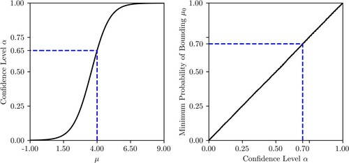
For example, the CD in Equation (2(2) $\mathrm{C}(\mu ,\mathit{x})=\mathrm{T}(\frac{\mu -{\mu }_x}{{\sigma }_{\mathit{x}}/\sqrt{n}};n-1),$(2) ) produces the Singh plot shown on the right side of Figure 1. The left of the figure demonstrates ${\mathrm{C}}^{\ast }(\mu ,\mathit{x})$ for one of the samples $\mathit{x}$. If this were a case where ${\mu }_0$ was not known precisely, the confidence level required to produce a one-sided interval using Equation (2(2) $\mathrm{C}(\mu ,\mathit{x})=\mathrm{T}(\frac{\mu -{\mu }_x}{{\sigma }_{\mathit{x}}/\sqrt{n}};n-1),$(2) ) which would bound it for this particular sample would have to be of an α-level of ${\mathrm{C}}^{\ast }({\mu }_0,\mathit{x})=0.65$ or greater, as indicated by the dotted blue line. The figure on the right extends this to $m={10}^4$ samples of the same distribution and indicates adherence to Equation (3(3) $\mathrm{P}({\mathrm{C}}^{-1}(\mathit{\alpha },\mathit{x}\sim \mathrm{F}({\theta }_0))\ni {\theta }_0)=\alpha ;\mathrm{\forall }\alpha \in [0,1].$(3) ) in that $\mathrm{P}({\mathrm{C}}^{\ast }(\mathit{\alpha },\mathit{x})\ni {\mu }_0)\approx \alpha ;\mathrm{\forall }\mathit{\alpha }\subseteq [0,1]$. For example, a confidence level of $\alpha =0.7$ is indicated on the plot with a dotted blue line, showing the true probability of coverage which in this case is 0.7.

Figure 1. (a) A single example of a proposed CD from Equation (2(2) $\mathrm{C}(\mu ,\mathit{x})=\mathrm{T}(\frac{\mu -{\mu }_x}{{\sigma }_{\mathit{x}}/\sqrt{n}};n-1),$(2) ) generated from $\mathit{x}=\{x_1,\dots ,x_{10}\}\sim \mathrm{N}({\mu }_0=4,\sigma =3)$. The confidence level required to bound the true mean ${\mu }_0$ in this example is shown as 0.65. (

, ${\mathrm{C}}^{\ast }(\mathit{\mu },\mathit{x})$;

, ${\mathrm{C}}^{\ast }({\mu }_0,\mathit{x})$). (b) Singh plot for the proposed CD about the same target distribution, generated from $m={10}^4$ samples $\mathit{X}=\{{\mathit{x}}_1,\dots ,{\mathit{x}}_m\}$ (

, $\mathrm{S}(\mathit{\alpha };{\mu }_0)$;

, $\mathrm{U}(0,1)$;

, $\mathrm{S}(\alpha =0.7;{\mu }_0)$).

There are deviations from the $\mathrm{U}(0,1)$ CDF, but these are slight. These deviations may be a result of sampling error. If the result is concerning and computational resources are available, a higher sample count may indicate whether this is the case. In this example the deviations are small, so it may not be unreasonable to accept this as evidence of maintaining confidence. If this needs to be quantified then a goodness-of-fit test may indicate whether these deviations are simply sampling error or an indication of an issue with the procedure.

These Singh plots give a clear visual cue as to the reliability of these CDs. The procedure maintains confidence if the ECDF of the confidence levels required to bound the true value in each of the m samples matches the U$(0,1)$ CDF.

The left of Figure 1 represents the CD for one possible sample that could be drawn from the target distribution. The value of 0.65 represents the minimum confidence required to cover the true value for this sample and forms part of the set of α-levels that generate the ECDF in the right of Figure 1. Note that this is a minimum requirement, so any level of confidence above this value would cover it as well and any values below would fail to do so. In this way, all confidence levels can be evaluated simultaneously for coverage. This is due to the nested nature of the CIs, (5) ${\mathrm{C}}^{-1}({\mathit{\alpha }}_1,\mathit{x})\subseteq {\mathrm{C}}^{-1}({\mathit{\alpha }}_2,\mathit{x});\mathrm{\forall }{\mathit{\alpha }}_1,{\mathit{\alpha }}_2\subseteq [0,1],{\mathit{\alpha }}_1\subseteq {\mathit{\alpha }}_2.$(5) A procedure could produce non-nested CIs, but these are counterintuitive. Increased confidence should not exclude values that would be included with lower confidence. And doing so would prevent the evaluation of all α-levels with each sample. Nested CIs that are unique for each α-level are required for Equation (5(5) ${\mathrm{C}}^{-1}({\mathit{\alpha }}_1,\mathit{x})\subseteq {\mathrm{C}}^{-1}({\mathit{\alpha }}_2,\mathit{x});\mathrm{\forall }{\mathit{\alpha }}_1,{\mathit{\alpha }}_2\subseteq [0,1],{\mathit{\alpha }}_1\subseteq {\mathit{\alpha }}_2.$(5) ) to apply and allow for efficient assessment.

Singh plots allow any proposed procedure to be quickly assessed to ensure that they are utilised from an informed perspective. The result in Figure 1 is shown for demonstrative purposes, this CD is known to perform at all α-levels. The utility of the Singh plot becomes apparent when used to assess the properties of procedures which may have been unknown or poorly understood properties.

4.1. Proposed Bernoulli confidence distribution Singh plot

A demonstration of a viable proposed distribution is shown in the preceding section, but what would visually indicate an invalid procedure? A simple example is that of inference about the rate parameter ${\theta }_0\in \mathrm{\Theta }$ of a Bernoulli distribution. A sample drawn from a Bernoulli process can be used to generate a Bayesian posterior for ${\theta }_0$ from a conjugate Jeffreys prior, taking the form of a beta distribution with parameters a = 0.5 and b = 0.5. This produces the following proposed CD for inference about the true parameter ${\theta }_0$ given a sample $\mathit{x}=\{x_1,\dots ,x_n\},x_i\sim \mathrm{Ber}(p={\theta }_0),$ where $\mathrm{Ber}(p)$ is a Bernoulli distribution with rate parameter p: (6) ${\mathrm{C}}^{\ast }(\theta ,\mathit{x})=\mathrm{B}(\theta ;a=\sum \mathit{x}+0.5,b=n-\sum \mathit{x}+0.5),$(6) where B$(\theta ;a,b)$ is the CDF of a beta distribution with parameters a, b evaluated at θ. Note that the confidence procedure will be additionally affected by the nature of a discrete distribution. For example, with a length n = 10 sample there are only 11 possible values of $\sum \mathit{x}$ for any θ. This means there are only 11 possible levels of confidence required to cover ${\theta }_0$ in any outcome, so any resulting Singh plot will be stepped. Because of this, a result such as that seen in Figure 1 would not be technically possible. However, with a sufficiently large sample size n it would asymptotically approach the U$(0,1)$ CDF. But the utility of inferential procedures such as these relies on performance with limited sample sizes, so a procedure should retain validity even at small sample sizes. Note that increasing the Singh plot sample count m would not remove the steps, it would simply produce a higher resolution Singh plot. For a demonstration of the impact of sample size on Singh plots from discrete distributions see Section 5 and Figure 5.

Equation (6(6) ${\mathrm{C}}^{\ast }(\theta ,\mathit{x})=\mathrm{B}(\theta ;a=\sum \mathit{x}+0.5,b=n-\sum \mathit{x}+0.5),$(6) ) can be assessed as a proposed CD in a similar manner as the distribution in Equation (2(2) $\mathrm{C}(\mu ,\mathit{x})=\mathrm{T}(\frac{\mu -{\mu }_x}{{\sigma }_{\mathit{x}}/\sqrt{n}};n-1),$(2) ). A collection of m sample sets are drawn from the target distribution and used to generate one-sided $[0,{\mathrm{C}}^{\ast }({\theta }_0,\mathit{x})]$ CIs. Again, ordering and plotting the confidence levels of these intervals produces a Singh plot, which can be quickly checked to confirm that coverage is maintained.

Figure 2 indicates that the proposed CD in Equation (6(6) ${\mathrm{C}}^{\ast }(\theta ,\mathit{x})=\mathrm{B}(\theta ;a=\sum \mathit{x}+0.5,b=n-\sum \mathit{x}+0.5),$(6) ) is not valid. This is due to the deviations from the desired bounding probability, as indicated by the Singh plot extending above and below the U$(0,1)$ CDF at many points. The deviations are clear, a quantitative assessment of goodness-of-fit is unlikely to be of any value here.

Figure 2. (a) A single example of a proposed CD from Equation (6(6) ${\mathrm{C}}^{\ast }(\theta ,\mathit{x})=\mathrm{B}(\theta ;a=\sum \mathit{x}+0.5,b=n-\sum \mathit{x}+0.5),$(6) ) generated from $\mathit{x}=\{x_1,\dots ,x_{10}\}\sim \mathrm{Ber}(p={\theta }_0)$. The confidence level required to bound the true rate ${\theta }_0$ is shown as 0.75. (

, ${\mathrm{C}}^{\ast }(\mathit{\theta },\mathit{x})$;

, ${\mathrm{C}}^{\ast }({\theta }_0,\mathit{x})$). (b) Singh plot for the proposed CD about the same target distribution, generated from $m={10}^4$ samples $\mathit{X}=\{{\mathit{x}}_1,\dots ,{\mathit{x}}_m\}$. (

, $\mathrm{S}(\mathit{\alpha };{\theta }_0)$;

, $\mathrm{U}(0,1)$;

, $\mathrm{S}(\alpha =0.7;{\theta }_0)$).

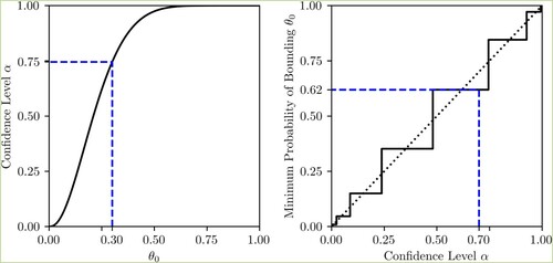
A confidence level of 0.7 is indicated on the right-hand plot with a dotted blue line as a point of comparison against other procedures. The actual coverage probability here is only 0.62, indicating that an $\alpha =0.70$ level CI would only bound the true value with a probability of $\approx 0.62$, a difference of $\approx -0.08$. Using this procedure as the basis for a decision could lead to unexpectedly frequent errors. In this case, a different procedure should be devised, or more data should be collected. As discussed earlier, with enough data this procedure approaches a point where the minimum difference may be considered negligible. For example, for a minimum difference of $\approx -0.01$ this procedure needs around $m={10}^4$ samples in the example given above. This is a representation of the reduced epistemic uncertainty in the problem due to an abundance of data. This effect is discussed further in Section 5.1.

4.2. Imprecise Bernoulli confidence distribution Singh plot

Since Equation (6(6) ${\mathrm{C}}^{\ast }(\theta ,\mathit{x})=\mathrm{B}(\theta ;a=\sum \mathit{x}+0.5,b=n-\sum \mathit{x}+0.5),$(6) ) failed to provide coverage, a different procedure must be devised. The discrete nature of the distribution prevents any CD from satisfying Equation (3(3) $\mathrm{P}({\mathrm{C}}^{-1}(\mathit{\alpha },\mathit{x}\sim \mathrm{F}({\theta }_0))\ni {\theta }_0)=\alpha ;\mathrm{\forall }\alpha \in [0,1].$(3) ). However, an acceptable alternative may be a distribution which satisfies a relaxed form: (7) $\mathrm{P}({\mathrm{C}}^{-1}(\mathit{\alpha },\mathit{x}\sim \mathrm{F}({\theta }_0))\ni {\theta }_0)\ge \alpha ;\mathrm{\forall }\alpha \in [0,1],$(7) which would guarantee a minimum rate of coverage, represented by a Singh plot which stochastically dominates U$(0,1)$. This would also allow the same minimum rate of coverage to be defined for a continuous distribution if Equation (3(3) $\mathrm{P}({\mathrm{C}}^{-1}(\mathit{\alpha },\mathit{x}\sim \mathrm{F}({\theta }_0))\ni {\theta }_0)=\alpha ;\mathrm{\forall }\alpha \in [0,1].$(3) ) cannot be satisfied. However, this raises an issue when considering intervals that are not one-sided, such as centred confidence intervals. A centred confidence interval derived from ${\mathit{\alpha }}_C=[\underset{\_}{\alpha },\overline{\alpha }]$ is a subset of a larger, one-sided interval derived from ${\mathit{\alpha }}_U=[0,\overline{\alpha }]$, where the excluded subset corresponds to ${\mathit{\alpha }}_L=[0,\underset{\_}{\alpha })$. These each define a set on Θ, for example ${\mathit{\theta }}_U={\mathrm{C}}^{-1}({\mathit{\alpha }}_U,\mathit{x})$. If a distribution satisfies Equation (7(7) $\mathrm{P}({\mathrm{C}}^{-1}(\mathit{\alpha },\mathit{x}\sim \mathrm{F}({\theta }_0))\ni {\theta }_0)\ge \alpha ;\mathrm{\forall }\alpha \in [0,1],$(7) ) then (8a) $\begin{array}{rl}{P}_U& =\mathrm{P}({\mathit{\theta }}_U\ni {\theta }_0)\ge \overline{\alpha }\in [\overline{\alpha },1],\end{array}$(8a) (8b) $\begin{array}{rl}\mathrm{and}{P}_L& =\mathrm{P}({\mathit{\theta }}_L\ni {\theta }_0)\ge \underset{\_}{\alpha }\in [\underset{\_}{\alpha },1].\end{array}$(8b) The probability of the true value being located within the central section ${\mathit{\theta }}_C={\mathit{\theta }}_U\cap {\mathit{\theta }}_L^C$ can then be calculated using interval arithmetic. Since ${\mathit{\theta }}_L\subseteq {\mathit{\theta }}_U$, then the probability of ${\theta }_0$ being contained within ${\mathit{\theta }}_C$ can be expressed as (9a) $\begin{array}{rl}{P}_C& =\mathrm{P}({\mathit{\theta }}_C\ni {\theta }_0)=P_U-P_L,\end{array}$(9a) (9b) $\begin{array}{rl}{P}_C& \in [0,1-\underset{\_}{\alpha }].\end{array}$(9b) In this case, it is possible that $P_C\le \overline{\alpha }-\underset{\_}{\alpha }$. Because of this any precise CD ${\mathrm{C}}^{-1}(\alpha ,\mathit{x})\in \mathrm{\Theta };\mathrm{\forall }\alpha \in [0,1]$ which satisfies Equation (7(7) $\mathrm{P}({\mathrm{C}}^{-1}(\mathit{\alpha },\mathit{x}\sim \mathrm{F}({\theta }_0))\ni {\theta }_0)\ge \alpha ;\mathrm{\forall }\alpha \in [0,1],$(7) ) but not Equation (3(3) $\mathrm{P}({\mathrm{C}}^{-1}(\mathit{\alpha },\mathit{x}\sim \mathrm{F}({\theta }_0))\ni {\theta }_0)=\alpha ;\mathrm{\forall }\alpha \in [0,1].$(3) ) cannot guarantee a minimum rate of coverage for intervals other than those that are one-sided. This can be remedied by considering imprecise methods. For demonstrative purposes, this article will consider imprecise CDs, or c-boxes [2].

With a c-box two precise CDFs are defined, ${\mathrm{C}}_U$ and ${\mathrm{C}}_L$, where ${\mathrm{C}}_U$ stochastically dominates ${\mathrm{C}}_L$. Because of this, ${\mathrm{C}}_U([0,\alpha ],\mathit{x})\subseteq {\mathrm{C}}_L([0,\alpha ],\mathit{x})$ and ${\mathrm{C}}^{-1}(\alpha ,\mathit{x})=[{\mathrm{C}}_U(\alpha ,\mathit{x}),{\mathrm{C}}_L(\alpha ,\mathit{x})]$. If an α-interval is used to define a CI with such a structure, defining ${\mathit{\theta }}_U={\mathrm{C}}_U([0,\overline{\alpha }],\mathit{x})$ and ${\mathit{\theta }}_L={\mathrm{C}}_L([0,\underset{\_}{\alpha }],\mathit{x})$ could result in a case where ${\mathit{\theta }}_U\subset {\mathit{\theta }}_L$, and therefore, $P_U<P_L$. This would imply that the probability $P_C=P_U-P_L$ can be negative. Defining ${\mathit{\theta }}_U={\mathrm{C}}_L(\overline{\alpha },\mathit{x})$ and ${\mathit{\theta }}_L={\mathrm{C}}_U(\underset{\_}{\alpha },\mathit{x})$ prevents this error. Equation (1(1) ${\mathrm{C}}^{-1}(\mathit{\alpha },\mathit{x})=[{\mathrm{C}}^{-1}(\underset{\_}{\alpha },\mathit{x}),{\mathrm{C}}^{-1}(\overline{\alpha },\mathit{x})],$(1) ) in this case becomes (10) ${\mathrm{C}}^{-1}(\mathit{\alpha },\mathit{x})=[{\mathrm{C}}_U^{-1}(\underset{\_}{\alpha },\mathit{x}),{\mathrm{C}}_L^{-1}(\overline{\alpha },\mathit{x})].$(10) If ${\mathrm{C}}_L$ satisfies Equation (7(7) $\mathrm{P}({\mathrm{C}}^{-1}(\mathit{\alpha },\mathit{x}\sim \mathrm{F}({\theta }_0))\ni {\theta }_0)\ge \alpha ;\mathrm{\forall }\alpha \in [0,1],$(7) ) then $P_C\ge \overline{\alpha }-\underset{\_}{\alpha }$ only if $P_L\in [0,\underset{\_}{\alpha })$. This can be achieved by ensuring that ${\mathrm{C}}_U$ satisfies (11) $\mathrm{P}({\mathrm{C}}_U^{-1}(\mathit{\alpha },\mathit{x}\sim \mathrm{F}({\theta }_0))\ni {\theta }_0)<\alpha ;\mathrm{\forall }\alpha \in [0,1].$(11) This can be achieved by defining $C_U$ in such a way that it will satisfy Equation (7(7) $\mathrm{P}({\mathrm{C}}^{-1}(\mathit{\alpha },\mathit{x}\sim \mathrm{F}({\theta }_0))\ni {\theta }_0)\ge \alpha ;\mathrm{\forall }\alpha \in [0,1],$(7) ) only for one-sided α intervals of the form $[\alpha ,1]$. One-sided α-intervals of the form $[0,\alpha ]$ will then have a coverage rate which satisfies Equation (11(11) $\mathrm{P}({\mathrm{C}}_U^{-1}(\mathit{\alpha },\mathit{x}\sim \mathrm{F}({\theta }_0))\ni {\theta }_0)<\alpha ;\mathrm{\forall }\alpha \in [0,1].$(11) ). With this, $P_L\in [0,\underset{\_}{\alpha })$ and, therefore, (12) $P_C={\mathrm{C}}_L({\mathit{\theta }}_U,\mathit{x})-{\mathrm{C}}_U({\mathit{\theta }}_L,\mathit{x})=[\overline{\alpha },1]-[0,\underset{\_}{\alpha })=(\overline{\alpha }-\underset{\_}{\alpha },1],$(12) which satisfies the requirement of minimum coverage probability defined in Equation (7(7) $\mathrm{P}({\mathrm{C}}^{-1}(\mathit{\alpha },\mathit{x}\sim \mathrm{F}({\theta }_0))\ni {\theta }_0)\ge \alpha ;\mathrm{\forall }\alpha \in [0,1],$(7) ).

For the Bernoulli distribution, Clopper–Pearson intervals allow each rate value θ to be assigned an interval confidence level ${\mathrm{C}}^{\ast }(\theta ,\mathit{x}):\theta \to \alpha \subseteq [0,1]$. This represents the interval of confidence levels required to cover the given value of θ for each distribution within the envelope of the Clopper–Pearson CDFs. Similarly, the inverse operation ${\mathrm{C}}^{-1\ast }(\alpha ,\mathit{x})=[\underset{\_}{\theta },\overline{\theta }]$ returns an interval of θ values that would be covered for each distribution within the envelope at the specified confidence level α. This is referred to as an imprecise CD or c-box.

The upper and lower CDs ${\mathrm{C}}_U^{\ast }(\cdot )$ and ${\mathrm{C}}_L^{\ast }(\cdot )$ of the c-box define $\overline{\alpha }$ and $\underset{\_}{\alpha }$, respectively, for each θ. In the case of the Clopper–Pearson c-box, these distributions are defined as follows: (13a) $\begin{array}{r}{\mathrm{C}}_L^{\ast }(\theta ,\mathit{x})=\mathrm{B}(\theta ;\sum \mathit{x}+1,n-\sum \mathit{x}),\end{array}$(13a) (13b) $\begin{array}{r}{\mathrm{C}}_U^{\ast }(\theta ,\mathit{x})=\mathrm{B}(\theta ;\sum \mathit{x},n-\sum \mathit{x}+1).\end{array}$(13b) The corresponding Singh plot in this case will need to account for both ${\mathrm{C}}_L$ and ${\mathrm{C}}_U$. The former must stochastically dominate U$(0,1)$, whilst the latter must be stochastically dominated by U$(0,1)$. Since the Singh plots are shown in Figure 3 for the upper and lower limit distributions of the c-box straddle, but never cross the U$(0,1)$ CDF, the imprecise CD is valid. This comes at the cost of wider intervals than the distribution proposed in Equation (6(6) ${\mathrm{C}}^{\ast }(\theta ,\mathit{x})=\mathrm{B}(\theta ;a=\sum \mathit{x}+0.5,b=n-\sum \mathit{x}+0.5),$(6) ), though this reflects the lack of information available in the data used for inference. The width of the output intervals will decrease as more information is available. Again, the left of Figure 3 indicates an example of an imprecise CD for one possible sample.

Figure 3. (a) A single example of a proposed CD from Equation (13) generated from $\mathit{x}=\{x_1,\dots ,x_{10}\}\sim \mathrm{Ber}(p={\theta }_0)$. The confidence level required to bound the true rate ${\theta }_0$ is shown as [0.05, 0.17]. (

, ${\mathrm{C}}_U^{\ast }(\mathit{\theta },\mathit{x})$;

, ${\mathrm{C}}_L^{\ast }(\mathit{\theta },\mathit{x})$;

, ${\mathrm{C}}^{\ast }({\theta }_0,\mathit{x})$). (b) Singh plot for the proposed CD about the same target distribution, generated from $m={10}^4$ samples $\mathit{X}=\{{\mathit{x}}_1,\dots ,{\mathit{x}}_m\}$. (

, ${\mathrm{S}}_U(\mathit{\alpha };{\theta }_0)$;

, ${\mathrm{S}}_L(\mathit{\alpha };{\theta }_0)$;

, $\mathrm{U}(0,1)$;

, $\mathrm{S}(\alpha =0.7;{\theta }_0)$).

4.3. Predictive confidence distributions

Singh plots can similarly be used to assess the confidence properties of predictive distributions. These function similarly to standard CDs used for inference, but they output prediction intervals guaranteed to bound the next realisation with a desired frequency rather than bounding some true parameter. There are a number of possible examples, but an interesting imprecise case is for non-parametric prediction of the next realisation $x_{n+1}$ given a sample of i.i.d. realisations $\mathit{x}=\{x_1,\dots ,x_n\}$.

The procedure for prediction is the same as for inference, though the confidence level required to bound the true subsequent realisation $\mathrm{C}(x_{n+1},\mathit{x})$ is calculated rather than one which provides coverage of any fixed parameter. The lower and upper limit CDs are defined as follows for the non-parametric prediction case: (14a) $\begin{array}{rl}{\mathrm{C}}_L^{\ast }(x_{n+1},\mathit{x})& =\frac{|\{x_i\in \mathit{x}:x_i\le x_{n+1}\}|}{n+1},\end{array}$(14a) (14b) $\begin{array}{rl}{\mathrm{C}}_U^{\ast }(x_{n+1},\mathit{x})& =1-\frac{|\{x_i\in \mathit{x}:x_i\ge x_{n+1}\}|}{n+1}.\end{array}$(14b) Again, the coverage properties of this procedure can be demonstrated using a Singh plot as shown in Figure 4, with a demonstration of the imprecise CD for one sample shown on the left. A Gaussian mixture distribution, $F(x)\sim 0.5N(4,3)+0.5N(5,1.5)$, is used here for demonstrative purposes.

Figure 4. (a) A single example of a proposed CD from Equation (14) generated from $\mathit{x}=\{x_1,\dots ,x_{10}\}\sim \mathrm{F}([{\mu }_1,{\mu }_2],[{\sigma }_1,{\sigma }_2])$ where $\mathrm{F}([{\mu }_1,{\mu }_2],[{\sigma }_1,{\sigma }_2])=0.5\cdot \mathrm{N}({\mu }_1=4,{\sigma }_1=3)+0.5\cdot \mathrm{N}({\mu }_2=5,{\sigma }_2=1.5)$. The confidence level required to bound the true value $x_{n+1}$ is shown as $\mathrm{C}({\mu }_0,\mathit{x})=[0.55,0.64]$. (

, ${\mathrm{C}}_U^{\ast }(\mathit{\theta },\mathit{x})$;

, ${\mathrm{C}}_L^{\ast }(\mathit{\theta },\mathit{x})$;

, ${\mathrm{C}}^{\ast }({\theta }_0,\mathit{x})$). (b) Singh plot for the proposed imprecise CD about the same target distribution, generated from $m={10}^4$ samples $\mathit{X}=\{{\mathit{x}}_1,\dots ,{\mathit{x}}_m\}$ (

, ${\mathrm{S}}_U(\mathit{\alpha };{\theta }_0)$;

, ${\mathrm{S}}_L(\mathit{\alpha };{\theta }_0)$;

, $\mathrm{U}(0,1)$;

, $\mathrm{S}(\alpha =0.7;\mathrm{F}([{\mu }_1,{\mu }_2],[{\sigma }_1,{\sigma }_2]))$).

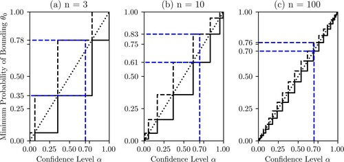
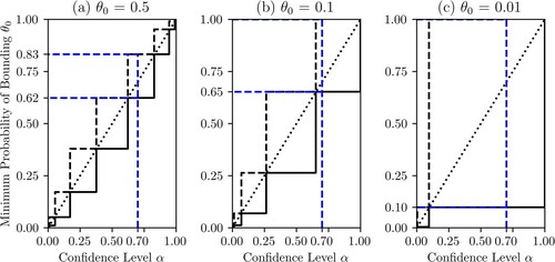
Figure 5. A series of Singh plots used for inference about ${\theta }_0=0.4$ generated using Equation (13) from $m={10}^4$ samples of varying length n (

, ${\mathrm{S}}_U(\mathit{\alpha };{\theta }_0)$;

, ${\mathrm{S}}_L(\mathit{\alpha };{\theta }_0)$;

, $\mathrm{U}(0,1)$;

, $\mathrm{S}(\alpha =0.7;{\theta }_0)$).

5. Representation of confidence procedure characteristics

Precise CDs are required to satisfy Equation (3(3) $\mathrm{P}({\mathrm{C}}^{-1}(\mathit{\alpha },\mathit{x}\sim \mathrm{F}({\theta }_0))\ni {\theta }_0)=\alpha ;\mathrm{\forall }\alpha \in [0,1].$(3) ) if they are to be used to draw anything other than one-sided intervals and should be consistent regardless of the sample size or parameters. Imprecise CDs, and precise CDs that are used solely for one-sided CIs, only need to satisfy Equation (7(7) $\mathrm{P}({\mathrm{C}}^{-1}(\mathit{\alpha },\mathit{x}\sim \mathrm{F}({\theta }_0))\ni {\theta }_0)\ge \alpha ;\mathrm{\forall }\alpha \in [0,1],$(7) ) and offer no such consistency, reflecting the epistemic uncertainty in the data. This section describes how these uncertainties present themselves in Singh plots when assessing one-sided or imprecise CDs.

5.1. Representing uncertainty from limited data

Figure 5 demonstrates how Singh plots for imprecise CDs differ when performed on various sample sizes. As the number of data points increases, the Singh plot converges to the perfect case, matching the U$(0,1)$ CDF. Lower sample sizes are shown to produce CIs which have coverage, but which are wider than they would be with more data. For example, with a sample size of n = 3, an $\alpha =0.7$ CI as indicated by the dotted blue line would have similar coverage properties to one with $\alpha =0.5$.

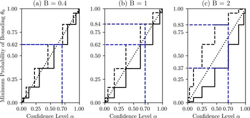
5.2. Representing uncertainty about rare events

Figure 6 demonstrates how Singh plots of Equation (6(6) ${\mathrm{C}}^{\ast }(\theta ,\mathit{x})=\mathrm{B}(\theta ;a=\sum \mathit{x}+0.5,b=n-\sum \mathit{x}+0.5),$(6) ) respond to varying rate ${\theta }_0$. Inferring the rate of a rare event with a small data set is naturally going to be difficult. This will be reflected in Singh plots as broad confidence regions. For example, an $\alpha =0.25$ CI is as likely to bound the true parameter ${\theta }_0=0.01$ as one with $\alpha =0.7$ as indicated by the dotted blue line. Increasing the sample size will converge these towards the U$(0,1)$ CDF as seen above, though a feature of note is that the Singh plot becomes asymmetric as ${\theta }_0$ deviates from the centre of the support $\theta =0.5$.

Figure 6. A series of Singh plots used for inference about a varying ${\theta }_0$ generated using Equation (13) from $m={10}^4$ samples of length n = 10 (

, ${\mathrm{S}}_U(\mathit{\alpha };{\theta }_0)$;

, ${\mathrm{S}}_L(\mathit{\alpha };{\theta }_0)$;

, $\mathrm{U}(0,1)$;

, $\mathrm{S}(\alpha =0.7;{\theta }_0)$).

5.3. Underconfidence and overconfidence

Since it is relatively simple to produce a Singh plot, they can be used to modify and assess CDs. One hope may be that through some modification, a CD may be developed which produces tighter bounds whilst preserving the property of coverage. For example, Equation (13) could be modified to alter the uncertainty expressed in the imprecise CD by changing the value that is added to generate each side of the interval. Equation (15) replaces the value of 1 in Equation (13) with a parameter c which controls the width of the α intervals: (15a) $\begin{array}{rl}{\alpha }_L& ={\mathrm{C}}_L^{\ast }(\theta ,\mathit{x})=\mathrm{B}(\theta ;\sum \mathit{x}+c,n-\sum \mathit{x}),\end{array}$(15a) (15b) $\begin{array}{rl}{\alpha }_U& ={\mathrm{C}}_U^{\ast }(\theta ,\mathit{x})=\mathrm{B}(\theta ;\sum \mathit{x},n-\sum \mathit{x}+c).\end{array}$(15b) This again produces proposed CDs, as the impact of this change is not yet known. The coverage impact of varying c can then be inspected through the use of Singh plots.

As can be seen in Figure 7, decreasing c below 1 produces an invalid c-box, as the Singh plots for both bounds clearly extend beyond the U$(0,1)$ CDF. This procedure is overconfident, CIs drawn from this procedure are not guaranteed to bound the true value at a minimum desired rate as demanded by Equation (7(7) $\mathrm{P}({\mathrm{C}}^{-1}(\mathit{\alpha },\mathit{x}\sim \mathrm{F}({\theta }_0))\ni {\theta }_0)\ge \alpha ;\mathrm{\forall }\alpha \in [0,1],$(7) ).

Figure 7. A series of Singh plots used for inference about ${\theta }_0=0.4$ generated using Equation (13) from $m={10}^4$ samples of length n = 10 sample with varying degrees of confidence demonstrated by altering the c parameter in Equation (15) (

, ${\mathrm{S}}_U(\mathit{\alpha };{\theta }_0)$;

, ${\mathrm{S}}_L(\mathit{\alpha };{\theta }_0)$;

, $\mathrm{U}(0,1)$;

, $\mathrm{S}(\alpha =0.7;{\theta }_0)$).

Increasing c does not produce an invalid procedure, but instead produces a procedure with additional imprecision. This procedure would be considered underconfident, as the CIs drawn from it bound the true value at a rate greater than but not equal to the confidence level used to generate them. It satisfies Equation (7(7) $\mathrm{P}({\mathrm{C}}^{-1}(\mathit{\alpha },\mathit{x}\sim \mathrm{F}({\theta }_0))\ni {\theta }_0)\ge \alpha ;\mathrm{\forall }\alpha \in [0,1],$(7) ), but ideally a more suitable procedure should be developed.

It should be noted that a procedure such as the case when c = 1 is considered conservative by many [4,8]. This is a comment on the fact that the width of the CIs it produces is often wide by comparison to many alternative procedures. Procedures could be compared based on the area between the ECDF and the $U(0,1)$ CDF. However, higher α-levels such as 0.95 are generally used in inference, so a more conservative procedure may be preferable if it allows for less conservatism at higher α-levels. Singh plots can guide the selection and assessment of the proposed procedures, but the selection of an optimal procedure is beyond the scope of this article.

5.4. Global coverage properties

Portraying the properties of an imprecise or one-sided procedure for a known ${\theta }_0$ allows for assessment of many characteristics but generally ${\theta }_0$ is unknown, hence the desire to infer its true value. In this case, a Singh plot can also portray the global coverage properties for unknown parameters within the support of the parameter Θ.

This is done by targeting an interval of interest on the support $\mathit{\theta }\in \mathrm{\Theta }$, sampling this region to generate a series of distributions $\mathit{F}=\{\mathrm{F}({\theta }_1),\dots ,\mathrm{F}({\theta }_k)\}$ where each $\mathrm{F}({\theta }_i)$ represents the CDF of the target distribution with parameter ${\theta }_i$. Each of these distributions may produce different Singh plots individually, as seen in Figure 6 where values of ${\theta }_0\ne 0.5$ introduce asymmetry in the Singh plot. Samples are generated for each of these distributions, individual Singh plots are calculated and then the lower bound of this second-order Singh plot is used as the final output, a global Singh plot sample $S_G$ which follows the distribution described in Equation (16(16) ${\mathrm{S}}_G(\mathit{\alpha },\mathit{\theta })=\underset{{\theta }_i\in \mathit{\theta }}{min}\{\mathrm{P}({\mathrm{C}}^{\ast -1}(\mathit{\alpha },\mathit{x}\sim \mathrm{F}({\theta }_i))\ni {\theta }_i)\}.$(16) ). The lower bound defines the minimum observed rate at which the specified α-level CI will bound the true value for all of the tested values of the target parameter. If this lower bound satisfies Equation (7(7) $\mathrm{P}({\mathrm{C}}^{-1}(\mathit{\alpha },\mathit{x}\sim \mathrm{F}({\theta }_0))\ni {\theta }_0)\ge \alpha ;\mathrm{\forall }\alpha \in [0,1],$(7) ) then the procedure can be used for the target interval with confidence that it will provide coverage for any value within the specified interval, though knowledge of conservatism is lost. This is a computationally expensive approach and may benefit from alterations to the Monte Carlo sampling process in order to identify values of θ which define the lower bound.

For a precise structure, or for a fixed confidence interval method (such as centred or one-sided intervals) with an imprecise structure, this is defined as (16) ${\mathrm{S}}_G(\mathit{\alpha },\mathit{\theta })=\underset{{\theta }_i\in \mathit{\theta }}{min}\{\mathrm{P}({\mathrm{C}}^{\ast -1}(\mathit{\alpha },\mathit{x}\sim \mathrm{F}({\theta }_i))\ni {\theta }_i)\}.$(16) The same can be defined generally for an imprecise structure, noting the requirement of the lower bound to be dominated by the uniform: (17) ${\mathrm{S}}_G(\mathit{\alpha },\mathit{\theta })\in [\underset{{\theta }_i\in \mathit{\theta }}{max}\{\mathrm{P}({\mathrm{C}}_L^{\ast -1}(\mathit{\alpha },\mathit{x})\ni {\theta }_i)\},\underset{{\theta }_i\in \mathit{\theta }}{min}\{\mathrm{P}({\mathrm{C}}_U^{\ast -1}(\mathit{\alpha },\mathit{x})\ni {\theta }_i))\}],$(17) where $\mathit{x}\sim \mathrm{F}({\theta }_i)$. This is demonstrated in Figure 8 with the procedure described in Equation (13), taking values of θ across the interval $[0,1]$. This demonstrates that the Clopper–Pearson c-box is capable of providing intervals with frequentist coverage regardless of the value of θ. An example of how to perform this for a precise one-sided procedure is given in Algorithm 2.

Figure 8. Global Singh plot produced using k = 100 θ values drawn from $[0,1]$, each producing $m={10}^4$ Monte Carlo samples using Equation (13) for inference about θ with a sample size of n = 10 (

, ${\mathrm{S}}_U(\mathit{\alpha };\mathit{\theta })$;

, ${\mathrm{S}}_L(\mathit{\alpha };\mathit{\theta })$;

, $\mathrm{U}(0,1)$;

, $\mathrm{S}(\alpha =0.7;{\theta }_0)$).

This algorithm can be used to assess an imprecise two-sided procedure by Equation (17(17) ${\mathrm{S}}_G(\mathit{\alpha },\mathit{\theta })\in [\underset{{\theta }_i\in \mathit{\theta }}{max}\{\mathrm{P}({\mathrm{C}}_L^{\ast -1}(\mathit{\alpha },\mathit{x})\ni {\theta }_i)\},\underset{{\theta }_i\in \mathit{\theta }}{min}\{\mathrm{P}({\mathrm{C}}_U^{\ast -1}(\mathit{\alpha },\mathit{x})\ni {\theta }_i))\}],$(17) ), replacing ${\alpha }_i=min({\alpha }_{1:k,i})$ with ${\alpha }_i=max({\alpha }_{1:k,i})$ for $S_U$. It should be noted that the sample size will also affect the inference about ${\theta }_i$. It is assumed that this procedure is applied to a case with a known sample size, otherwise an exhaustive representation of the minimum coverage probability would have to be calculated by sampling combinations of $(\theta ,n)$. Similarly, nuisance parameters may be treated in a similar manner, though the most efficient means of doing so will vary depending on the procedure being assessed. Calculating Singh plots with variations in the nuisance parameters may indicate whether their effect on the minimum confidence required is monotone, and if so end-points could be taken to reduce computational cost.

6. Chebyshev UCL coverage

Most of the above examples are demonstrations of known confidence procedures or of clearly deficient suggestions. However, the value of Singh plots lies in visual demonstrations of the performance of procedures where the deficiencies are not known.

As an example, the ProUCL package is a software package for statistical analysis of environmental datasets, and one of the statistics that can be calculated is the upper confidence limit of the mean of a population, $\overline{\mu }\in \mathbb{R}$. This could be used for calculation of the upper confidence limit on the expected value of the concentration of a particular pollutant in water samples, amongst many other use cases. The software documentation notes the difficulty of handling skewed datasets and suggests the use of an estimator based on the Chebyshev inequality, as defined below [9]: (18) $\overline{{\mathrm{C}}^{\ast }}(\mathit{\alpha },\mathit{x})={\mu }_{\mathit{x}}+\frac{{\sigma }_{\mathit{x}}}{\sqrt{n}}\sqrt{\frac{1}{1-\alpha }-1}.$(18) The novelty of this upper confidence limit is the claim that it is a reasonable non-parametric estimator, that is, it should be correct regardless of the underlying distribution. This is an excellent quality for an estimator to have, though the documentation of ProUCL does note that highly skewed datasets may lose coverage, and that in such cases the data should be inspected to ensure that there is truly only a single population being reported. This raises questions about how skewness affects the coverage, and is it really reasonable to simply raise or lower the required α-level to get an appropriate CI?

Singh plots can serve here as a tool for inspecting the properties of this estimator in an intuitive manner. A family of distributions can be generated to ‘stress test’ the provided estimator. In this case, scaled Bernoulli distributions represent a family of distributions which should be particularly difficult for such an estimator to maintain coverage. The estimator relies on scaling the standard deviation of a sample, and there are many samples that can be drawn with a high probability from a highly skewed Bernoulli process which have zero standard deviation. The Bernoulli parameter θ here can be manipulated to alter the skewness of the distribution in order to observe how highly skewed datasets affect the coverage of this confidence limit.

The PRoUCL version 5.1.0 documentation defines ‘extremely skewed’ as data where the standard deviation of the log-transformed data ${\hat{\sigma }}_{\mathit{x}}$ is greater than 3. For a Bernoulli distribution, this statistic is inverse to the observed skewness since the maximum standard deviation will be observed where $\theta =0.5$ and the distribution has no skewness.

Firstly Equation (18(18) $\overline{{\mathrm{C}}^{\ast }}(\mathit{\alpha },\mathit{x})={\mu }_{\mathit{x}}+\frac{{\sigma }_{\mathit{x}}}{\sqrt{n}}\sqrt{\frac{1}{1-\alpha }-1}.$(18) ) must be inverted to map $\mu \in \mathbb{R}$ onto $[0,1]$. This gives the following equation: (19) ${\overline{{\mathrm{C}}^{\ast }}}^{-1}(\mu ,\mathit{x})=1-{({\left(\frac{\sqrt{n}(\overline{\mu }-{\mu }_{\mathit{x}})}{{\sigma }_{\mathit{x}}}\right)}^2+1)}^{-1}.$(19) This can then be used to generate a Singh plot for a variety of Bernoulli distributions with skewness controlled by the parameter θ. According to the ProUCL documentation, it should be expected that the procedure provides coverage for moderately skewed data, but that this may not hold for highly skewed data. Although the proposed CD is precise, it produces one-sided intervals, so the procedure could be considered valid if the Singh plot satisfies Equation (7(7) $\mathrm{P}({\mathrm{C}}^{-1}(\mathit{\alpha },\mathit{x}\sim \mathrm{F}({\theta }_0))\ni {\theta }_0)\ge \alpha ;\mathrm{\forall }\alpha \in [0,1],$(7) ).

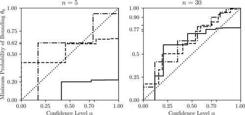
Figure 9 indicates that for small sample sizes, Equation (18(18) $\overline{{\mathrm{C}}^{\ast }}(\mathit{\alpha },\mathit{x})={\mu }_{\mathit{x}}+\frac{{\sigma }_{\mathit{x}}}{\sqrt{n}}\sqrt{\frac{1}{1-\alpha }-1}.$(18) ) fails to provide coverage at all confidence levels even for the unskewed Bernoulli distribution ($\theta =0.5$, skewness = 0). Any skew in the dataset detracts further from the ability to provide coverage. This can be offset with a larger sample size, though even with 30 realisations, skewed data $(\theta =0.05$, skewness = 4.13) leads to a lack of coverage. As such, Equation (18(18) $\overline{{\mathrm{C}}^{\ast }}(\mathit{\alpha },\mathit{x})={\mu }_{\mathit{x}}+\frac{{\sigma }_{\mathit{x}}}{\sqrt{n}}\sqrt{\frac{1}{1-\alpha }-1}.$(18) ) should not be considered for use on small datasets, particularly those which may be skewed. A $\alpha =0.7$ CI from this procedure cannot be guaranteed to bound the true mean with a rate of at least 0.7. In the $\theta =0.2$ case (skewness=1.5) with a sample size of $n=5,$ for example, an $\alpha =0.7$ CI would bound the true mean with a frequency of only 0.62. These coverage figures also only apply to the particular distributions they are applied to. In practice, the utility of this estimator comes from its supposed applicability to non-parametric cases. This is a one-sided precise distribution, so the rate at which an α-level CI will bound the true value will change with the underlying distribution. Because of this, attempting to suggest a lower α-level in order to be more accurate to the true coverage, or a higher α-level to try and be more conservative would not be justifiable.

Figure 9. Singh plots representing the coverage probability for a desired α confidence level interval using Equation (19(19) ${\overline{{\mathrm{C}}^{\ast }}}^{-1}(\mu ,\mathit{x})=1-{({\left(\frac{\sqrt{n}(\overline{\mu }-{\mu }_{\mathit{x}})}{{\sigma }_{\mathit{x}}}\right)}^2+1)}^{-1}.$(19) ) for inference about data generated from Bernoulli distributions with varying θ-parameters. Two plots are shown, for sample sizes of n = 5 (left) and n = 30 (right), each produced from $m={10}^4$ samples (

, $\mathrm{S}(\mathit{\alpha };{\theta }_0=0.05)$;

, $\mathrm{S}(\mathit{\alpha };{\theta }_0=0.2)$;

, $\mathrm{S}(\mathit{\alpha };{\theta }_0=0.5)$;

, $\mathrm{U}(0,1)$).

This upper confidence limit estimator may be of some use, but it is in no way a distribution-free estimator and should not be used for these purposes when sample sizes are small. However, Singh plots may be a means of determining the limits of its use as a confidence estimator, and in this case, it appears that increasing the sample size allows for confidence on mildly skewed datasets. Whether the underconfidence and the potential for losing applicability to highly skewed datasets are acceptable is a matter of choice. But that choice can be easily informed by the creation of a Singh plot.

7. Conclusion

Singh plots, whilst not technically capable of providing strict proof of coverage, represent an intuitive and simple means of portraying the coverage properties of confidence procedures, both precise and imprecise. They allow for comparisons against different proposed procedures, as well as the analysis of general and specific cases for inference and prediction.

Confidence procedures are a widely applicable means of providing probabilistic statements, and Singh plots allow for their use and development without requiring specialist knowledge regarding their formulation. This allows for more widespread adoption and development of this robust approach to uncertainty quantification. This is particularly relevant for the development of procedures suitable for calculating with confidence procedures.

Disclosure statement

No potential conflict of interest was reported by the author(s).

Additional information

Funding

This work was supported by EPSRC and ESRC Centre for Doctoral Training in Quantification and Management of Risk & Uncertainty in Complex Systems & Environments [Grant EP/L015927/1]; and EPSRC Digital twins for improved dynamic design [Grant EP/R006768/1].

References

- Schweder T, Hjort NL. Confidence and likelihood. Scand J Statist. 2002;29(2):309–332.
- Ferson S, O'Rawe J, Balch M. Computing with confidence: imprecise posteriors and predictive distributions. In: Proceedings of the 2nd International Conference on Vulnerability and Risk Analysis and Management (ICVRAM) and the 6th International Symposium on Uncertainty Modeling and Analysis (ISUMA); 2014 July 13–16; Liverpool. Reston (VA): American Society of Civil Engineers; 2014. p. 895–904.
- Balch MS. Mathematical foundations for a theory of confidence structures. Int J Approx Reason. 2012;53(7):1003–1019.
- Singh K, Xie M, Strawderman WE. Confidence distribution (CD): distribution estimator of a parameter. Lecture Notes-Monograph Series. 2007;54:132–150.
- Student. The probable error of a mean. Biometrika. 1908;1:1–25.
- Babu GJ. Kesar Singhs contributions to statistical methodology. Stat Methodol. 2014;20:2–10.
- Hoo ZH, Candlish J, Teare D. What is an ROC curve? Emerg Med J. 2017;34:357–359.
- Balch MS. New two-sided confidence intervals for binomial inference derived using Walley's imprecise posterior likelihood as a test statistic. Int J Approx Reason. 2020;123:77–98.
- Singh A, Maichle R, Lee SE. On the computation of a 95% upper confidence limit of the unknown population mean based upon data sets with below detection limit observations. Las Vegas: U.S. Environmental Protection Agency (EPA); 2006. (EPA Publication; no. EPA/600/R-06/022).