A data-driven kernel estimator of the density function

Abstract

The main purpose of this paper is to provide an effective nonparametric method of kernel estimation of the density function for various specific data. A convex linear combination of the most locally effective known kernel estimators constructed using different approaches allows one to build an estimator that combines the best features of all analysed estimators. The paper presents an original concept for studying the local effectiveness of the kernel estimator of the density function based on the Marczewski–Steinhaus metric. It is shown that none of the applied kernel estimators can be considered globally optimal if local effectiveness is taken into account. The presented numerical calculations were done for experimental data recording groundwater levels on a melioration facility and supported by simulation studies.

KEYWORDS:

• Kernel density estimation
• nonparametric statistics
• hydrology
• effectiveness of estimators
• simulations

Introduction

In the statistics literature, many forms of kernel estimators of density functions for a given random sample X₁, X_2, ..,X_n are known (e.g. [1–5]). The construction of these estimators was based on various analytical and numerical approaches. In the papers [6,7] Karczewski and Michalski considered eight kernel estimators ${\hat{f}}_n$of the density function f in the form ${\hat{f}}_n(x)=\frac{1}{nh}\sum _{i=1}^{n}K\left(\frac{x-X_i}{h}\right),$where h is the window width, also called the smoothing parameter or bandwidth, and K is a real positive function integrable to 1 as a kernel of estimator ${\hat{f}}_n$ . The authors considered two kernels:

a Gaussian kernel and the kernel given by Epanechnikov, using several methods: Silverman’s rule of thumb, the Sheather–Jones method, cross-validation methods and other more known plug-in methods. From a theoretical point of view, the most important features of kernel estimators are strong consistency, asymptotic unbiasedness and uniform convergence [2] and optimal choice of the smoothing bandwidth.

For assessing the effectiveness of the considered estimates and their similarity, we applied a distance measure for measurable and integrable functions proposed by Marczewski and Steinhaus in 1958 [8]. The reference point for testing the effectiveness of selected estimators was the frequency histogram at the intervals indicated, e.g. by the experimenter. In the numerical analysis, the structure of the frequency histogram was flexible as needed. The analysed estimators showed a different effectiveness depending on the selected interval and it was impossible to select the most effective estimator for all given intervals.

In this paper, we propose a new data-driven kernel estimator (DDKE) in the form of a convex linear combination of the locally most effective kernel estimators, i.e. the construction of this estimator involves the analysed estimators that showed the best efficiency for each of the examined intervals.

Methods – construction of a data-driven kernel estimator

The starting point for the construction of the data-driven kernel estimator (DDKE) is the selection of a set of kernel estimators ${\hat{f}}_n$of the density function f from a certain wider class of kernel estimators of a density function. The results of testing the effectiveness of the considered kernel estimators led to the selection of eight different estimators: ${\hat{f}}_1$ – Silverman’s [9], ${\hat{f}}_2$ – Sheather & Jones [5], ${\hat{f}}_3$ – unbiased cross-validation, ${\hat{f}}_4$ – biased cross-validation [4,5], ${\hat{f}}_5$ – Altman & Leger [1], ${\hat{f}}_6$ – Bowman with Gaussian kernel, ${\hat{f}}_7$ – Bowman with Epanechnikov kernel [3,10], ${\hat{f}}_8$ – Polansky & Baker [11]. It should be noted, however, that at the beginning of this procedure, one can start with any reasonable set of estimators which are not necessarily kernel density function, i.e.: $S_1=\{{\hat{f}}_i:i=1,\dots ,k\}$(in our case k = 8).

Now, let’s define a set of intervals $[x_i,x_{i+1}]$ for i = 0, … , m, (x₀=  min and x_m+1= max, in our example m = 14) covering each of the lines that make up the frequency polygon ${\hat{f}}_0$, and the set $S_2$ of estimators ${\hat{f}}_i\in S_1$ which in the i-th interval turned out to be the most effective, i.e. $S_2=\{{\hat{f}}_i:i=1,\dots ,m;{\hat{f}}_i\in S_1\}.$ For the most efficient estimator of consideration we accept the one that reaches the shortest distance in relation to the empirical frequency polygon when using the Marczewski–Steinhaus metric, defined as below ${\sigma }_{\mu }(f,g)=\frac{\int |f(x)-g(x)|d\mu (x)}{\int max(|f(x)|,|g(x)|)d\mu (x)}$for non-negative and integrable functions f and g [8].

Finally, we create a convex linear combination of the estimators ${\hat{f}}_i$ of the form: (1) $DDKE(x)=\sum _{i=0}^m{\alpha }_i(x){\hat{f}}_i$(1) for weights ${\alpha }_i(x)$ defined as follows ${\alpha }_i(x)=\frac{{\beta }_i(x)}{{\sum }_{i=0}^n{\beta }_i(x)},\text{ where }{\beta }_i(x)=\frac{1}{{(x_i-x)}^2+{(x_{i+1}-x)}^2}.$

The downside of this approach was the potential to choose a version of the kernel density estimator that has the lowest M-S distance in a single interval but a potentially bad fit outside of it. This could lead to suboptimal overall performance. To combat that, an additional rule was introduced. The estimator ${\hat{f}}_i$ can only be a part of a linear combination if its average M-S distance over all intervals is not higher than 150% of smallest mean distance among all chosen estimators.

Note

In the past, attempts were made to create a linear combination of kernel estimators [12]. The approach presented in this paper takes into account the local fit of the estimator to the data, which in turn allows the creation of an estimator as a convex linear combination of the analysed estimators with the i-th weights inversely proportional to the distance of point $x$ from the edges of interval $[x_i,x_{i+1}].$The method proposed in this article shows some similarity to the methods that use the smoothing parameter h (x), which depends on the argument x with the constant kernel K instead of the constant parameter h and methods for determining the asymptotic mean integrated squared error (AMISE (h))[13,14].

Analysis was performed for real hydrological data recording groundwater levels on a melioration facility [7,15] as well as on simulated datasets created from mixtures of density functions. Calculations were performed in R for Windows software [16]. Kernel estimation was performed using the kedd [17] and kerdiest [18] packages.

Results and conclusions

In this section, the behaviour of DDKE is presented for both real and simulated data. An important goal of these analyses was to investigate the sensitivity of the DDKE estimator to the multimodality of the estimated density function. Once the concept of a mode is defined, the question arises whether an observed mode in a density estimate really arises from a corresponding feature in the assumed underlying density [9]. The study of the effectiveness of kernel estimators strongly related to empirical data has serious consequences with effects on possible forecasts, which is of paramount importance for a researcher of a given phenomenon. In this section, we present the numerical calculations performed for the data from the real experiment and additionally for the simulation data, for a mixture of probability distributions of the type beta and further for a mixture of two-parameter gamma distributions with appropriate shape and scale parameters.

Experimental data

In this example, we use groundwater level data from melioration studies on the foothill object Długopole. Daily registered groundwater levels were averaged based on measurements from a dozen or so piezometers suitably located at the research station. The experimental data are derived from the Institute of Agricultural and Forest Improvement of Wroclaw University of Environmental and Life Sciences (currently). The data set includes the groundwater level measurements for specified ranges of levels from 10 to 150 cm, taken every 10 cm. The experimental data aggregated in a frequency table were reproduced by repeated use of a random number generator with a given frequency structure.

Table 1 shows the matrix of distances d(${\hat{f}}_{\text{i}},{\hat{f}}_0$) calculated according to the Marczewski–Steinhaus metric between the kernel estimator ${\hat{f}}_{\text{i}}$ and the frequency polygon ${\hat{f}}_0$ built on the empirical data. Additionally, the first row shows the bandwidth calculated for each base kernel estimator and the last row shows the average distance (D) from all intervals, respectively. On the basis of the calculated distances d(${\hat{f}}_{\text{i}},{\hat{f}}_0$), for each of the determined intervals $[x_i,x_{i+1}]$, the most effective estimator ${\hat{f}}_{\text{i}}$ was selected. Then, based on the set of the most effective local estimators, a linear combination was created according to the formula (1). In this example, the following estimators have been selected: Bowman with Gaussian kernel, Sheather & Jones and Bowman estimator with Epanechnikov kernel. The DDKE achieved the shortest distance for 4 out of 15 intervals (including two without a clear advantage). In other cases, the differences between the approach we proposed and the most effective estimator were relatively small and satisfy the assumption of an acceptable sufficiently small distance Δ from the minimum distance [12]. Additionally, the determined combination of estimators showed the greatest efficiency globally, that is over the entire range of the studied variability, and has the lowest mean error in the individual intervals. Figure 1.

Figure 1. Comparison of the DDKE and locally most effective kernel density estimators for the Długopole dataset.

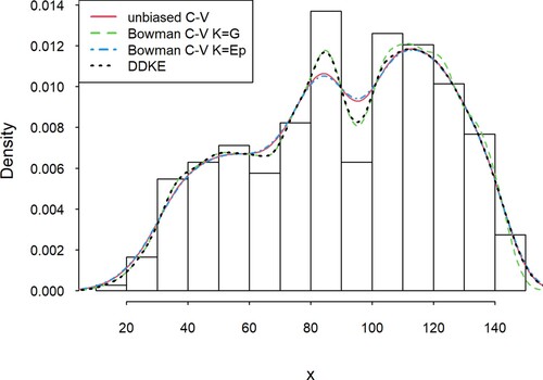
Table 1. Matrix of distances d(${\hat{f}}_i,{\hat{f}}_0$) calculated according to the Marczewski–Steinhaus metric for each interval, averaged over all intervals and bandwidth of each estimator – Długopole dataset. Estimators used for DDKE marked in bold.

	Silverman	unbiased C-V	biased C-V	Altman & Leger	Bowman C-V K = G.	Bowman C-V K = E.	Polansky & Baker	Sheather & Jones	DDKE
Bandwidth	8.65	6.7	10.95	6.21	4.48	7.05	6.5	8.27	–
5 – 15	0.606	0.438	0.729	0.386	0.191	0.473	0.417	0.549	0.196
15–25	0.293	0.176	0.389	0.142	0.052	0.199	0.162	0.251	0.053
25–35	0.112	0.093	0.131	0.087	0.077	0.097	0.090	0.105	0.074
35–45	0.086	0.054	0.123	0.045	0.019	0.059	0.050	0.074	0.016
45–55	0.043	0.027	0.063	0.023	0.016	0.030	0.025	0.037	0.016
55–65	0.080	0.064	0.095	0.060	0.051	0.067	0.062	0.074	0.053
65- 75	0.121	0.097	0.134	0.089	0.060	0.102	0.094	0.113	0.066
75- 85	0.129	0.100	0.153	0.091	0.060	0.106	0.096	0.119	0.060
85- 95	0.162	0.136	0.176	0.125	0.069	0.142	0.132	0.154	0.075
95–105	0.133	0.109	0.145	0.101	0.053	0.115	0.106	0.126	0.068
105–115	0.081	0.056	0.107	0.050	0.028	0.061	0.054	0.073	0.058
115–125	0.014	0.019	0.046	0.023	0.040	0.017	0.021	0.014	0.017
125–135	0.013	0.019	0.042	0.021	0.024	0.018	0.020	0.014	0.019
135–145	0.046	0.032	0.068	0.035	0.066	0.033	0.033	0.038	0.035
145–155	0.236	0.086	0.383	0.126	0.403	0.078	0.099	0.163	0.084
Average D	0.174	0.100	0.186	0.094	0.081	0.106	0.097	0.127	0.059

The proposed hybrid model can also be modified by generalizing ${\beta }_i(x)=\frac{1}{{(x_i-x)}^{2l}+{(x_{i+1}-x)}^{2l}},l\in N.$This change increases the impact of the most effective local estimator in relation to the estimators from other intervals. In our examples, however, this change had little effect on the fit.

Illustrative example – beta mixture

In this example, a sample size of 200 was generated from a mixture of two beta density functions f(x, p, q) with parameters (p, q) = (10, 30) and (p, q) = (3, 3) and equal weights for both. To make the intervals clear, the values were multiplied by 140. Table 2, similarly to Table 1, shows the matrix of Marczewski–Steinhaus distances for intervals of 10 lengths, an average of all intervals for every kernel density estimation and bandwidth calculated for each base kernel estimator (Figure 2).

Figure 2. Comparison of the DDKE and locally most effective kernel density estimators for the simulated data (beta mixture).

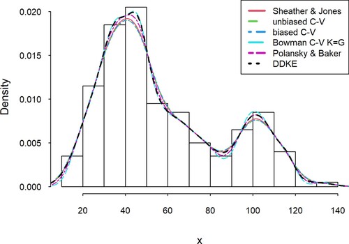
Table 2. Matrix of distances d(${\hat{f}}_i,{\hat{f}}_0$) calculated according to the Marczewski–Steinhaus metric for each interval, averaged over all intervals and bandwidth of each estimator – simulated dataset (beta mixture). Estimators used for DDKE marked in bold.

	Silverman	unbiased C-V	biased C-V	Altman & Leger	Bowman C-V K = G.	Bowman C-V K = E.	Polansky & Baker	Sheather & JonesP}	DDKE
Bandwidth	8.83	6.48	6.47	5.18	4.19	8.99	5.09	6.12	–
5 – 15	0.319	0.086	0.086	0.180	0.327	0.332	0.192	0.092	0.098
15–25	0.053	0.027	0.027	0.028	0.031	0.055	0.028	0.027	0.036
25–35	0.053	0.012	0.012	0.015	0.031	0.056	0.016	0.009	0.021
35–45	0.110	0.044	0.043	0.016	0.012	0.114	0.015	0.035	0.015
45–55	0.098	0.067	0.067	0.047	0.038	0.099	0.045	0.062	0.032
55–65	0.100	0.075	0.074	0.063	0.058	0.102	0.062	0.071	0.062
65- 75	0.044	0.053	0.053	0.053	0.047	0.044	0.053	0.053	0.053
75- 85	0.164	0.094	0.094	0.065	0.077	0.169	0.064	0.085	0.074
85- 95	0.082	0.043	0.043	0.082	0.141	0.085	0.087	0.048	0.065
95–105	0.123	0.038	0.038	0.054	0.086	0.128	0.057	0.037	0.048
105–115	0.122	0.071	0.071	0.057	0.059	0.126	0.057	0.066	0.068
115–125	0.267	0.188	0.188	0.139	0.105	0.271	0.135	0.175	0.124
125–135	0.709	0.607	0.606	0.490	0.378	0.714	0.479	0.581	0.537
135–145	0.218	0.308	0.308	0.318	0.362	0.206	0.321	0.309	0.330
Average D	0.172	0.108	0.108	0.099	0.107	0.177	0.099	0.103	0.095

Illustrative example – gamma mixture

For this example, a sample size of 200 was generated from a mixture of two gamma density functions f(x, p, λ) with parameters (p, λ) =  (5, 4) and (p, λ) =  (13, 3) and equal weights for both, and multiplied by 12. Table 3 shows the matrix of Marczewski–Steinhaus distances for intervals of 5 lengths, an average of all intervals for every kernel density estimation and bandwidth calculated for each base kernel estimator (Figure 3).

Figure 3. Comparison of the DDKE and locally most effective kernel density estimators for the simulated data (gamma mixture).

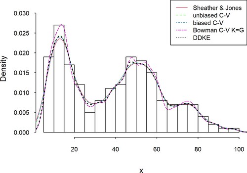
Table 3. Matrix of distances d(${\hat{f}}_i,{\hat{f}}_0$) calculated according to the Marczewski–Steinhaus metric for each interval, averaged over all intervals and bandwidth of each estimator – simulated dataset (gamma mixture). Estimators used for DDKE marked in bold.

	Silverman	unbiased C-V	biased C-V	Altman & Leger	Bowman C-V K = G.	Bowman C-V K = E.	Polansky & Baker	Sheather & Jones	DDKE
Bandwidth	7.23	3.54	3.68	3.74	2.32	6.03	3.72	3.9	–
0 – 5	0.283	0.152	0.160	0.163	0.101	0.254	0.162	0.172	0.093
5–10	0.300	0.075	0.085	0.089	0.014	0.238	0.087	0.100	0.056
10–15	0.204	0.056	0.055	0.055	0.110	0.140	0.055	0.056	0.058
15–20	0.033	0.058	0.055	0.053	0.100	0.036	0.054	0.050	0.053
20–25	0.254	0.101	0.101	0.100	0.105	0.193	0.100	0.100	0.092
25–30	0.321	0.115	0.120	0.122	0.083	0.250	0.121	0.127	0.118
30- 35	0.061	0.093	0.089	0.087	0.138	0.029	0.088	0.082	0.113
35- 40	0.057	0.050	0.051	0.051	0.029	0.051	0.051	0.052	0.037
40- 45	0.091	0.048	0.051	0.052	0.012	0.078	0.052	0.055	0.021
45–50	0.152	0.058	0.061	0.063	0.046	0.119	0.062	0.066	0.045
50–55	0.098	0.017	0.015	0.014	0.043	0.067	0.014	0.012	0.016
55–60	0.098	0.085	0.082	0.081	0.114	0.087	0.082	0.079	0.092
60–65	0.221	0.070	0.067	0.067	0.156	0.179	0.067	0.066	0.067
65–70	0.091	0.040	0.036	0.033	0.062	0.051	0.034	0.028	0.026
70 - 75	0.081	0.033	0.029	0.027	0.086	0.071	0.028	0.025	0.039
75–80	0.089	0.033	0.034	0.035	0.038	0.076	0.035	0.036	0.026
80–85	0.145	0.034	0.028	0.026	0.115	0.113	0.027	0.022	0.078
85–90	0.303	0.120	0.125	0.127	0.108	0.242	0.126	0.133	0.122
90–95	0.194	0.129	0.132	0.134	0.112	0.160	0.133	0.136	0.099
95–100	0.240	0.235	0.241	0.242	0.177	0.239	0.242	0.247	0.164
Average D	0.162	0.072	0.072	0.073	0.083	0.128	0.072	0.074	0.066

Among the eight considered estimators, four had at least one interval with minimal M-S distance; Unbiased CV twice, Biased CV twice, Bowman’s CV on gaussian kernel nine times and Sheater–Jones nine times. DDKE was optimal in seven of those intervals (0–5, 20–25, 45–50, 65–70, 90–95, 95–100), but it excelled in the average distance among all intervals. This illustrates that while it may not necessarily be best for every small interval, it eliminates the potential problematic local range each kernel density could have.

Simulation study

Additionally, a simulation study based on five hundred replications of a sample size of two hundred was performed. Twenty-eight distribution functions discussed by Berlinet and Devroy [2] implemented in ‘Benchden’ R package [19] were considered. To assess global accuracy, nine kernel density estimators are compared using averaged Marczewski–Steinhaus distance, and average integrates squared error (AISE). DDKE was calculated separately for both measures since in each case we consider different definitions of estimator effectiveness.

Tables 4 and 5 show that DDKE outperformed the remaining considered estimators both in terms of Marczewski–Steinhaus distance and AISE. In some cases, e.g. symmetric Pareto distribution, the effectiveness was very similar to that of kernel estimators that were used to build DDKE. This is linked to situations where most of analysed intervals have the same optimal estimator.

Table 4. Average Marczewski–Steinhaus distances with standard error times 10³ for 28 types of density functions. Calculations were performed on 500 replications with n = 200.

	Silverman	unbiased C-V	biased C-V	Altman & Leger	Bowman C-V K = G.	Bowman C-V K = E.	Polansky & Baker	Sheather & Jones	DDKE
Uniform	105.55	86.3	121.96	84.83	88.49	135.24	84.5	94.52	70.31
	(1.31)	(1.96)	(1.64)	(1.11)	(2.41)	(2.22)	(1.15)	(1.24)	(1.05)
Exponential	193.61	376.18	209.77	250.72	520.65	428.52	273.34	266.43	182.48
	(7.1)	(8.85)	(7.75)	(8.2)	(6.87)	(11.2)	(8.5)	(8.6)	(7.27)
Maxwell	105.75	115.52	89.96	129.84	137.29	133.01	126.05	101.68	75.91
	(2.14)	(4.5)	(2.24)	(2.62)	(4.46)	(3.81)	(2.53)	(2.46)	(1.81)
Double exponential	217.18	246.35	182.02	257.06	284.63	206.66	256.95	228.87	153.65
	(5.88)	(7.64)	(5.76)	(5.96)	(8.73)	(7.31)	(6.15)	(6.3)	(5.28)
Logistic	149.17	163.43	146.96	165.63	184.1	205.04	161.16	148.74	117.41
	(5.22)	(5.67)	(4.16)	(5.8)	(7.18)	(5.06)	(5.76)	(5.02)	(3.62)
Cauchy	927.41	925.49	771.24	887.81	898.44	815.02	933.8	930.27	731.08
	(5.1)	(4.6)	(8.69)	(5.47)	(5.42)	(10.4)	(4.5)	(4.85)	(9.8)
Extreme value	158.41	170.81	152.18	180.33	198.86	193.75	180.1	160.83	119.7
	(4.51)	(5.39)	(4.1)	(5.7)	(7.3)	(5.73)	(5.67)	(4.61)	(4.07)
Infinite peak	154.88	246.4	173.92	102.62	384.82	381.95	104.37	107.89	96.27
	(1.48)	(2.61)	(2.43)	(1.11)	(1.99)	(2.66)	(1.21)	(1.46)	(0.985)
Pareto	986.39	968.07	790.88	873.93	958.53	958.53	987.36	987.49	868.68
	(0.834)	(1.88)	(8.91)	(5.08)	(1.98)	(1.98)	(0.707)	(0.7)	(10.9)
Symmetric Pareto	986.97	974.39	878.55	899.35	952.54	889.93	987.23	987.24	871.18
	(0.658)	(1.12)	(6.42)	(7.76)	(2.91)	(9.07)	(0.644)	(0.643)	(10.3)
Normal	109.57	129.56	129.06	110.66	124.78	198.83	108.48	120.06	92.68
	(2.41)	(2.99)	(2.56)	(2.49)	(4.05)	(4.29)	(2.43)	(2.56)	(2.17)
Lognormal	405.59	560.81	462.74	475.11	641.68	561	538.55	520.96	399.6
	(13)	(10.4)	(12.6)	(11)	(7.72)	(12.7)	(12.5)	(11.5)	(13.1)
Uniform scale mixture	249.91	364.54	256.44	253.21	475.24	377.53	327.51	313.91	227.43
	(3.54)	(3.68)	(2.99)	(2.37)	(4.35)	(7.83)	(2.87)	(2.87)	(3.38)
Matterhorn	159.57	383.27	217.19	167.12	240.89	139.71	341.75	429.24	109.15
	(3.83)	(2.39)	(2.01)	(2.01)	(5.23)	(3.17)	(5.16)	(5.12)	(1.37)
Logarithmic peak	113.05	222.81	118.87	106.5	365.06	268.35	107.91	109.45	81.33
	(1.38)	(5.22)	(2.01)	(1.65)	(6.88)	(8.69)	(1.72)	(1.92)	(1.23)
Isosceles triangle	80.25	102.25	101.39	78.16	89.04	155.97	77.35	95.03	67.72
Isosceles triangle	(1.55)	(2.56)	(1.85)	(1.4)	(3.04)	(3.29)	(1.42)	(1.84)	(1.29)
Beta	79.81	94.79	100.52	73.49	80.23	145.14	74.37	94.49	66.81
	(1.57)	(2.04)	(1.82)	(1.36)	(2.08)	(2.37)	(1.42)	(1.78)	(1.33)
Chi-squared	301.29	585.01	268.25	400.03	627.21	627.21	488.59	517.87	245.48
	(8.18)	(6.08)	(7.12)	(8.17)	(4.21)	(4.21)	(8.29)	(8.05)	(7.27)
Normal cubed	812.28	814.03	437.69	716.61	748.74	617.49	857.32	867.53	430.35
	(4.78)	(3.85)	(8.25)	(6.12)	(6.9)	(12)	(3.06)	(2.69)	(8.33)
Inverse exponential	985.62	966.59	786.04	870.11	956.93	956.93	986.73	986.91	868.34
	(0.921)	(1.94)	(9.11)	(5.08)	(2.07)	(2.07)	(0.771)	(0.759)	(11.4)
Marronite	700.16	781.42	729.38	598.58	820.7	757.93	731.05	733.27	593.94
	(0.659)	(1.44)	(0.522)	(1.45)	(1.8)	(4.29)	(1.52)	(1.63)	(1.3)
Skewed binomial	121.47	131.26	150.02	112.52	130.07	187.66	110.59	115.32	92.74
	(2.66)	(3.57)	(2.97)	(2.48)	(3.8)	(3.96)	(2.45)	(2.5)	(2.27)
Claw	128.87	370.32	131.95	160.38	271.16	234.31	148.11	134.59	109.25
	(2.88)	(5.47)	(3.09)	(3.37)	(10.2)	(7.18)	(3.21)	(3.25)	(2.78)
Smooth comb	273.87	300.65	196.16	135.34	290.29	174.9	145.69	144.47	118.37
	(2.29)	(4.5)	(5.87)	(1.46)	(6.14)	(5.25)	(1.69)	(1.77)	(1.45)
Caliper	97	286.25	124.29	151.8	289.08	180.37	119.67	160.05	75.27
	(1.65)	(4.59)	(2.06)	(2.13)	(7.58)	(6.54)	(1.93)	(2.98)	(1.21)
Trimodal uniform	668.64	883.9	631.63	650.9	961.75	961.75	907.97	933.77	593.14
	(9.77)	(23.2)	(0.443)	(2.24)	(0.0325)	(0.0325)	(2.29)	(2.06)	(1.16)
Sawtooth	102.83	310.92	121.45	78.04	328	161.85	75.94	88.25	67.41
	(1.32)	(5.73)	(1.58)	(1.1)	(6.72)	(6.1)	(1.11)	(1.22)	(1.25)
Bilogarithmic peak	160.63	136.71	169.88	96.23	237.74	174.36	92.25	97.6	78.59
Bilogarithmic peak	(1.53)	(3.77)	(2.86)	(1.16)	(7.7)	(7.38)	(1.13)	(1.14)	(1.3)

Table 5. AISE with standard error times 10³ for 28 types of density functions. Calculations were performed on 500 replications with n = 200.

	Silverman	unbiased C-V	biased C-V	Altman & Leger	Bowman C-V K = G.	Bowman C-V K = E.	Polansky & Baker	Sheather & Jones	DDKE
Uniform	3.13	3.87	3.39	3.18	3.82	4.07	3.17	3.19	2.35
	(0.0578)	(0.132)	(0.052)	(0.0707)	(0.197)	(0.142)	(0.071)	(0.0658)	(0.0487)
Exponential	5.68	3.5	5.43	3.95	4.8	4.09	3.73	3.82	2.41
	(0.0919)	(0.0738)	(0.119)	(0.0667)	(0.12)	(0.106)	(0.065)	(0.0685)	(0.0568)
Maxwell	0.86	1.17	0.87	1.02	1.27	1.68	0.97	0.91	0.68
	(0.0364)	(0.0767)	(0.0362)	(0.044)	(0.106)	(0.0873)	(0.0413)	(0.0399)	(0.0313)
Double exponential	0.52	0.63	0.61	0.53	0.75	1.09	0.54	0.54	0.44
	(0.0202)	(0.0281)	(0.024)	(0.0205)	(0.0466)	(0.0483)	(0.0208)	(0.0212)	(0.0186)
Logistic	0.21	0.27	0.2	0.25	0.33	0.42	0.24	0.22	0.16
	(0.00991)	(0.0162)	(0.0103)	(0.0116)	(0.0267)	(0.0226)	(0.0112)	(0.0108)	(0.0091)
Cauchy	73.66	2.17	8.33	4.39	4.07	6.31	126.17	91.61	1.69
	(45.9)	(0.333)	(0.526)	(0.438)	(0.419)	(0.473)	(72.1)	(50.2)	(0.34)
Extreme value	0.37	0.47	0.39	0.43	0.58	0.79	0.43	0.39	0.31
	(0.0178)	(0.0264)	(0.0189)	(0.0196)	(0.0445)	(0.0442)	(0.0192)	(0.0188)	(0.0162)
Infinite peak	65.23	41.6	67.69	55.48	46.29	46.23	54.82	54.13	27.23
	(0.142)	(0.272)	(0.234)	(0.191)	(0.474)	(0.474)	(0.204)	(0.244)	(0.29)
Pareto	124368.78	0.93	1.04	1.01	0.95	0.95	1751838.6	2767410.5	0.57
	(111000)	(0.274)	(0.313)	(0.305)	(0.286)	(0.286)	(1590000)	(2520000)	(0.196)
Symmetric Pareto	94011.67	0.7	0.92	0.85	0.8	0.88	290088.47	269596.27	0.57
	(75000)	(0.163)	(0.217)	(0.2)	(0.188)	(0.208)	(203000)	(174000)	(0.137)
Normal	0.34	0.41	0.31	0.41	0.51	0.54	0.38	0.34	0.25
	(0.0158)	(0.0268)	(0.0157)	(0.0186)	(0.0389)	(0.0274)	(0.0178)	(0.0171)	(0.0137)
Lognormal	2.78	1.36	2.11	1.82	1.69	1.54	1.32	1.4	1.05
	(0.0743)	(0.0436)	(0.104)	(0.0586)	(0.0525)	(0.0505)	(0.0411)	(0.0437)	(0.0371)
Uniform scale mixture	3.34	2.52	3.31	3.17	3.08	3.03	2.59	2.67	2.06
	(0.0731)	(0.0347)	(0.0895)	(0.0387)	(0.0489)	(0.0687)	(0.0353)	(0.0355)	(0.032)
Matterhorn	240.81	390.55	235.74	231.69	263.84	231.22	371.75	572.81	163(1.4
	(4.44)	(7.97)	(0.786)	(2.43)	(5.79)	(3.45)	(16.9)	(29.6)	8)
Logarithmic peak	36.65	22.84	37.32	27.33	31.1	26.76	27.16	27.16	16.38
	(0.268)	(0.311)	(0.429)	(0.277)	(0.566)	(0.548)	(0.28)	(0.303)	(0.297)
Isosceles triangle	0.88	1.16	0.76	1.09	1.3	1.39	0.99	0.88	0.62
	(0.0378)	(0.0873)	(0.0328)	(0.0486)	(0.119)	(0.118)	(0.0447)	(0.041)	(0.028)
Beta	1.63	1.88	1.4	1.96	2.14	2.05	1.83	1.54	1.1
	(0.0782)	(0.123)	(0.0664)	(0.0978)	(0.16)	(0.0761)	(0.0922)	(0.08)	(0.052)
Chi-squared	35.59	20.16	40.8	29.53	18.59	18.59	24.91	23.42	18.25
	(0.797)	(0.452)	(0.933)	(0.674)	(0.383)	(0.383)	(0.59)	(0.554)	(0.412)
Normal cubed	36.19	36.42	62.11	48.01	43.37	51.49	29.62	35.04	22.16
	(3.85)	(3.86)	(5.55)	(4.85)	(4.45)	(4.96)	(2.68)	(2.85)	(2.5)
Inverse exponential	162172.06	1.05	1.13	1.1	1.06	1.06	2338405.13	4644881.66	0.51
	(114000)	(0.65)	(0.74)	(0.716)	(0.672)	(0.672)	(1620000)	(3320000)	(0.241)
Marronite	12.28	2.17	13.42	6.4	1.16	2.69	3.47	3.41	1.13
	(0.0311)	(0.0168)	(0.0182)	(0.0225)	(0.0403)	(0.0996)	(0.016)	(0.0265)	(0.0391)
Skewed binomial	0.58	0.67	0.73	0.54	0.63	0.95	0.53	0.57	0.42
	(0.0175)	(0.0299)	(0.017)	(0.0195)	(0.0287)	(0.027)	(0.019)	(0.0196)	(0.0157)
Claw	4.42	2.33	4.56	4.12	3.43	4.31	4.25	4.41	2.15
	(0.0424)	(0.0616)	(0.0417)	(0.0408)	(0.0902)	(0.0837)	(0.0427)	(0.0438)	(0.0516)
Smooth comb	5.03	1.68	3.86	2.51	1.85	2.64	2.33	2.36	1.29
	(0.0241)	(0.0316)	(0.115)	(0.0262)	(0.0494)	(0.0551)	(0.027)	(0.0296)	(0.0262)
Caliper	14.7	7.83	16.34	9.83	8.98	10.91	11.59	9.79	6.4
	(0.0943)	(0.122)	(0.11)	(0.106)	(0.218)	(0.243)	(0.116)	(0.151)	(0.0981)
Trimodal uniform	137.63	124.21	143.19	139	102.64	102.64	121.56	113.09	98.21
	(0.615)	(0.0175)	(0.00998)	(0.0574)	(0.088)	(0.088)	(1)	(1.31)	(0.727)
Sawtooth	1.73	0.75	1.75	1.73	0.85	1.2	1.73	1.74	0.65
	(0.00284)	(0.0237)	(0.00253)	(0.0035)	(0.028)	(0.0248)	(0.00352)	(0.00328)	(0.014)
Bilogarithmic peak	11.85	9.64	12.69	9.66	16.3	12.85	9.51	9.73	5.95
	(0.0806)	(0.159)	(0.118)	(0.0981)	(0.59)	(0.491)	(0.0993)	(0.102)	(0.114)

Discussion

The DDKE, a linear combination of selected kernel estimators, although not necessarily always locally optimal, provides us with the best overall efficiency in the average value of local efficiency relative to the frequency polygon. In addition, in the ranges where the estimator DDKE did not reach the minimum distance compared to the single estimators, the differences were usually not notable.

An important structural element of the presented method is its flexibility, related to a variable smoothing window and a different division, range of variability of the examined features into classes (e.g. groundwater level, as in this paper). Thus, to obtain better prognostic effects, the DDKE algorithm allows for a variable number of classes in which the local efficiency of the estimators is determined. Additionally, the width of the histogram bins does not need to be of the same length.

The method of determining the DDKE shows a certain computational complexity, as it includes two stages: the first one – selecting various kernel estimators (analysis of similarity of objects) and the second one – examining the local behaviour of the selected estimators in the specific ranges of variability of a given feature (efficiency analysis according to the indicated pattern).

Kernel estimation as a nonparametric estimation method is free from additional assumptions, in regard to the class of density function or its parameters. Additionally, kernel estimators have been researched for a long time and there is quite extensive literature on them (e.g. [2,5,9,20]), hence the decision to base construction of DDKE primarily on kernel estimators.

This method achieves the greatest benefits when the unknown probability distribution in the study of a certain phenomenon, e.g. hydrological or meteorological, is a distribution that is difficult to analyse due to multimodality and heavy tails. In such cases, it can be expected that the DDKE will include significantly different single estimators with different analytical properties – this effect is known in the determination of a mixed strategy under various restrictions in game theory. It is worth noting that the DDKE approach is not tied to any base estimator listed in this paper, and could be built on any density function including more complex estimators, focused on dealing with certain distribution characteristics [21,22]. It can also use measures other than the Marczewski–Steinhaus distance e.g. AISE, as shown in simulation study, which only adds to the method robustness.

The authors realize that the method of constructing a hybrid estimator proposed in this paper is only a certain alternative for achieving relatively good practical goals. At the same time, it is a challenge to harness estimation methods that are more robust to various peculiarities of unknown probability distributions governing a given phenomenon, e.g. the double kernel method [23] or the bootstrap method [2].

Disclosure statement

No potential competing interest was reported by the authors.

References

- Altman N, Léger C. Bandwidth selection for kernel distribution function estimation. J Stat Plan Inference. 1995;46:195–214.
- Berlinet A, Devroye L. A comparison of kernel density estimates. Publ L’Institut Stat L’Université Paris. 1994;38:3–59.
- Bowman AW. An alternative method of cross-validation for the smoothing of density estimates. Biometrika. 1984;71:353–360.
- Scott DW, Terrell GR. Biased and unbiased cross-validation in density estimation. J Am Stat Assoc. 1987;82:1131–1146.
- Givens GH, Hoeting JA. Computational statistics. 1st ed. New Jersey: John Wiley & Sons inc; 2005.
- Karczewski M, Michalski A. The study and comparison of one-dimensional kernel estimators – a new approach. Part 1. Theory and methods. ITM Web Conf. 2018;23:00017.
- Karczewski M, Michalski A. The study and comparison of one-dimensional kernel estimators – a new approach. Part 2. A hydrology case study. ITM Web Conf. 2018;23:00018.
- Marczewski E, Steinhaus H. On a certain distance of sets and the corresponding distance of functions. Colloq Math. 1958;6:319–327.
- Silverman BW. Density estimation: For statistics and data analysis. London: Chapman & Hall; 1986.
- Bowman A, Hall P, Prvan T. Bandwidth selection for the smoothing of distribution functions. Biometrika. 1998;85:799–808.
- Polansky AM, Baker ER. Multistage plug-in bandwidth selection for kernel distribution function estimates. J Stat Comput Simul. 2000;65:63–80.
- Rigollet P, Tsybakov AB. Linear and convex aggregation of density estimators. Math Methods Stat. 2007;16:260–280.
- Breiman L, Meisel W, Purcell E. Variable kernel estimates of multivariate densities. Technometrics. 1977;19:135–144.
- Hall P. On global properties of variable bandwidth density estimators. Ann Stat. 1992;20:762–778.
- Michalski A. The use of kernel estimators to determine the distribution of groundwater level. Meteorol Hydrol Water Manag. 2016;4:41–46.
- R Core Team. (2020). R: A Language and Environment for Statistical Computing [Internet]. Vienna, Austria; Available from: https://www.r-project.org/.
- Guidoum AC. Kernel estimator and bandwidth selection for density and its derivatives [Internet]. 2013 [cited 2020 Dec 29]. p. 1–22. Available from: https://cran.r-project.org/package=kedd.
- Quintela-del-Río A, Estévez-Pérez G. Nonparametric kernel distribution function estimation with kerdiest: an R package for bandwidth choice and applications. J Stat Softw. 2012;50(8):1–21.
- Mildenberger T, Weinert H. The Benchden package: benchmark densities for nonparametric density estimation. J Stat Softw. 2012;46:2–14.
- Wand MP, Jones MC. Kernel smoothing. biometrics. London: Chapman & Hall; 1995.
- Buch-Larsen T, Nielsen JP, Guillén M, et al. Kernel density estimation for heavy-tailed distributions using the champernowne transformation. Statistics (Ber. 2005;39:503–516.
- Jiang M, Provost SB. A hybrid bandwidth selection methodology for kernel density estimation. J Stat Comput Simul. 2014;84:614–627.
- Devroye L. The double kernel method in density estimation. Ann. l’I.H.P. Probab. Stat. 1989;25:533–580.