Computational issues in parameter estimation for hidden Markov models with template model builder

Abstract

A popular way to estimate the parameters of a hidden Markov model (HMM) is direct numerical maximization (DNM) of the (log-)likelihood function. The advantages of employing the TMB [Kristensen K, Nielsen A, Berg C, et al. TMB: automatic differentiation and Laplace approximation. J Stat Softw Articles. 2016;70(5):1–21] framework in R for this purpose were illustrated recently [Bacri T, Berentsen GD, Bulla J, et al. A gentle tutorial on accelerated parameter and confidence interval estimation for hidden Markov models using template model builder. Biom J. 2022 Oct;64(7):1260–1288]. In this paper, we present extensions of these results in two directions. First, we present a practical way to obtain uncertainty estimates in form of confidence intervals (CIs) for the so-called smoothing probabilities at moderate computational and programming effort via TMB. Our approach thus permits to avoid computer-intensive bootstrap methods. By means of several examples, we illustrate patterns present for the derived CIs. Secondly, we investigate the performance of popular optimizers available in R when estimating HMMs via DNM. Hereby, our focus lies on the potential benefits of employing TMB. Investigated criteria via a number of simulation studies are convergence speed, accuracy, and the impact of (poor) initial values. Our findings suggest that all optimizers considered benefit in terms of speed from using the gradient supplied by TMB. When supplying both gradient and Hessian from TMB, the number of iterations reduces, suggesting a more efficient convergence to the maximum of the log-likelihood. Last, we briefly point out potential advantages of a hybrid approach.

Keywords:

• Hidden Markov model
• template model builder
• smoothing probabilities
• confidence intervals
• maximum likelihood estimation
• robustness
• initial conditions

1. Introduction

Hidden Markov models (HMMs) are a well-studied and popular class of models in many areas. While they have been used for speech recognition historically [see, e.g. 1–5], these models also became important in many other fields due to their flexibility. These are, to name only a few, biology and bioinformatics [6–8], finance [9], ecology [10], stochastic weather modelling [11,12], and engineering [13]. In short, HMMs are a class of models where the given data is assumed to follow varying distributions according to an underlying unknown Markov chain. Parameter estimation for HMMs is typically achieved either by the Baum-Welch (BW) algorithm [3,14–17] – an Expectation–Maximization(EM)-type algorithm – or in a quite straightforward fashion by direct numerical maximization (DNM) of the (log-)likelihood function [see, e.g. 18,19]. A discussion of both approaches can be found in [20, p. 358]. Furthermore, [21] points out that it is challenging to fit complex models with the BW algorithm, [22, pp.  77–78] advises using DNM with HMMs due to the ease of fitting complex models, and [18,23] report a greater speed of DNM compared to the BW algorithm. The arguments of [24] point in a similar direction, underlining the often increased amount of mathematical and programming labor required by the EM algorithm, in particular for non-standard models. Nevertheless, the BW is highly accepted and finds widespread application. However, we will only use DNM in the following due to the possibility of accelerating the estimation via the R-package TMB [25,26].

In this paper, we present a straightforward procedure to calculate uncertainty estimates of the smoothing probabilities through appropriate use of TMB. Hence, we quantify the uncertainty of the state classifications of the observations at a low computational cost. To the best of our knowledge, such results on confidence intervals for the aforementioned probabilities are not available in the literature. Furthermore, the chosen optimization routine for DNM plays an important role in parameter estimation. While e.g. [22] focuses on the unconstrained optimizer nlm, alternatives include the popular nlminb [27] and many others, such as those provided by the optim function [28]. In this context, [29] compare different estimation routines for two-state HMMs: a Newton-Type algorithm [30,31], the Nelder–Mead algorithm [32], BW, and a hybrid algorithm successively executing BW and DNM. To complement these studies, we investigate the speed of several optimization algorithms, many of which allow the gradient and Hessian of the objective function as input. Particular focus lies on the ability of the TMB framework, which allows for easy retrieval of the exact gradient and Hessian (up to machine precision). This enriches the existing literature on parameter estimation for HMMs. Among others, Zucchini et al. [22] report that ‘Depending on the starting values, it can easily happen that the algorithm (i.e. DNM) identifies a local, but not the global, maximum’. The literature on how to tackle this problem is rich, and includes among others: the use of artificial neural networks to guess the initial values [33], model induction [34], genetic algorithms in combination with HMMs [35], hybridizing both the BW and the DNM algorithms [21,29,36], specific assumptions on the parameters [37], educated guesses [22, p. 53], and short EM-runs with 10 iterations or (model-based) clustering [38]. We investigate how stable the various considered optimization routines are towards poor initial values. Again, this part takes under consideration the special features of TMB, which have not been investigated yet. In this context, it is noteworthy that the recently developed R-package hmmTMB [see 39] provides a framework for working with HMMs and TMB. This package offers the choice between various optimization routines with the Nelder-Mead algorithm as default. Hence, our results may also provide guidance for users of hmmTMB.

The paper is organized as follows. In Section 2, we provide a brief overview of parameter estimation for HMMs, including inference for CIs. In Section 3 we show how uncertainty estimates of the smoothing probabilities can be computed via TMB. Then, we apply our results to a couple of data sets with different characteristics. We perform simulation studies in Section 4 to compare measures of performance and accuracy of various optimizers. In Section 5, we check how well these optimizers perform in the presence of poor initial values. Section 6 provides some concluding remarks. All code necessary to reproduce our results is available in the supporting information.

2. Basics on hidden Markov models

The HMMs considered here are fit on observed time series $\{X_t:t=1,\dots ,T\}$ where t denotes the (time) index ranging from one to T. In this setting, a mixture of conditional distributions is assumed to be driven by an unobserved (hidden) homogeneous Markov chain, whose states will be denoted as $\{C_t:t=1,\dots ,T\}$. We will use different conditional distributions in the paper. First, we specify an m-state Poisson HMM, i.e. with the conditional distribution $p_i(x)=\mathrm{P}(X_t=x|C_t=i)=\frac{{\mathrm{e}}^{-{\lambda }_i}{\lambda }_i^x}{x!}$with parameters ${\lambda }_i,i=1,\dots ,m$. Secondly, we consider Gaussian HMMs with conditional distribution specified by $p_i(x)=\mathrm{P}(X_t=x|C_t=i)=\frac{1}{\sigma \sqrt{2\pi }}{\mathrm{e}}^{-\frac{1}{2}{\left(\frac{x-{\mu }_i}{{\sigma }_i}\right)}^2},$with parameters $({\mu }_i,{\sigma }_i),i=1,\dots ,m$. In addition, $\mathbf{\Gamma }=\{{\gamma }_{ij}\},i,j=1,\dots ,m$ denotes the transition probability matrix (TPM) of the HMM's underlying Markov chain, and $\mathit{\delta }$ is a vector of length m collecting the corresponding stationary distribution. We assume that the Markov chains underlying our HMMs are irreducible and aperiodic. This ensures the existence and uniqueness of a stationary distribution as the limiting distribution [40]. However, these results are of limited relevance for most estimation algorithms, because the elements of $\mathbf{\Gamma }$ are generally strictly positive. Nevertheless, one should be careful when manually fixing selected elements of $\mathbf{\Gamma }$ to zero.

The basis for our estimation procedure is the (log-)likelihood function. We denote the ‘history’ of observations $x_t$ and the observed process $X_t$ up to time t by ${\mathit{x}}^{\mathbf{(}\mathit{t}\mathbf{)}}=\{x_1,\dots ,x_t\}$ and ${\mathit{X}}^{\mathbf{(}\mathit{t}\mathbf{)}}=\{X_1,\dots ,X_t\}$, respectively. In addition, let $\mathit{\theta }$ be the vector of model parameters. As explained, e.g. by Zucchini et al. [22, p. 37], the likelihood function can then be represented as a product of matrices: (1) $L(\mathit{\theta })=\mathrm{P}({\mathit{X}}^{\mathbf{(}\mathit{T}\mathbf{)}}={\mathit{x}}^{\mathbf{(}\mathit{T}\mathbf{)}})=\mathit{\delta }\mathit{P}(x_1)\mathbf{\Gamma }\mathit{P}(x_2)\mathbf{\Gamma }\mathit{P}(x_3)\dots \mathbf{\Gamma }\mathit{P}(x_T){\mathbf{1}}^{\prime },$(1) where the m conditional probability density functions evaluated at x (we use this term for discrete support as well) are collected in the diagonal matrix $\mathit{P}(x)=\left(\begin{array}{cccc}{p}_1(x)& & & 0\\ & p_2(x)& & \\ & & \ddots & \\ 0& & & p_m(x)\end{array}\right),$and ${\mathbf{1}}^{\prime }$ and $\mathit{\delta }$ denote a transposed vector of ones and the stationary distribution, respectively. That is, we assume that the initial distribution corresponds to $\mathit{\delta }$. The likelihood function given in Equation (1(1) $L(\mathit{\theta })=\mathrm{P}({\mathit{X}}^{\mathbf{(}\mathit{T}\mathbf{)}}={\mathit{x}}^{\mathbf{(}\mathit{T}\mathbf{)}})=\mathit{\delta }\mathit{P}(x_1)\mathbf{\Gamma }\mathit{P}(x_2)\mathbf{\Gamma }\mathit{P}(x_3)\dots \mathbf{\Gamma }\mathit{P}(x_T){\mathbf{1}}^{\prime },$(1) ) can be efficiently evaluated by a so-called forward pass through the observations, as illustrated in Appendix 1. Consequently, it is possible to obtain $\hat{\mathit{\theta }}$, the ML estimates of $\mathit{\theta }$, by -- in our case - unconstrained DNM. Since several of our parameters are constrained, we rely on known re-parametrization procedures (see Appendix 2 for details).

Confidence intervals (CIs) for the estimated parameters of HMMs can be derived via various approaches. The most common ones are Wald-type, profile likelihood, and bootstrap-based CIs. Bacri et al. [26] shows that TMB can yield valid Wald-type CIs in a fraction of the time required by classical bootstrap-based methods as investigated e.g. by Bulla and Berzel [29] and Zucchini et al. [22]. Furthermore, the likelihood profile method may fail to provide CIs [26]. Therefore, we rely on Wald-type confidence intervals derived via TMB. For details, see Appendix 3.

3. Uncertainty of smoothing probabilities

When interpreting the estimation results of an HMM, the so-called smoothing probabilities often play an important role. These quantities, denoted by $p_{it}(\mathit{\theta })$ in the following, correspond to the probability of being in state i at time t given the observations, i.e. $p_{it}(\mathit{\theta })={\mathrm{P}}_{\mathit{\theta }}(C_t=i|X^{(T)}=x^{(T)})=\frac{{\alpha }_t(i){\beta }_t(i)}{L(\mathit{\theta })},$and can be calculated for $i=1,\dots ,m$ and $t=1,\dots ,T$ [see, e.g. 22, p. 87]. The involved quantities ${\alpha }_t(i)$ and ${\beta }_t(i)$, which also depend on $\mathit{\theta }$, result directly from the forward- and backward algorithm, respectively, as illustrated in Appendix 1. Estimates of $p_{it}(\mathit{\theta })$ are obtained by $p_{it}(\hat{\mathit{\theta }})$ where $\hat{\mathit{\theta }}$ is the ML estimate of $\mathit{\theta }$.

An important feature of TMB is that it not only permits obtaining standard errors for $\hat{\mathit{\theta }}$ (and CIs for $\mathit{\theta }$), but in principle also for any other quantity depending on the parameters. This is achieved by combining the delta method with automatic differentiation (see Section A.1 in Appendix 3 for details). A minor requirement for deriving standard deviations for $p_{it}(\hat{\mathit{\theta }})$ via the ADREPORT function provided by TMB consists in implementing the function $p_{it}(\mathit{\theta })=g(\mathit{\psi })$ in C++. Then, this part has to be integrated into the scripts necessary for the parameter estimation procedure. It is noteworthy that, once implemented, the procedures related to inference of the smoothing probabilities do not need to change when the HMM considered changes, because the input vector for $p_{it}(\mathit{\theta })$ remains the same. The C++ code in the supporting information illustrates how to complete these tasks. Note that population value we are interested in constructing a CI for is $p_{it}(\mathit{\theta })$, which should not be confused with $E_{X^{(T)}}(P_{\hat{\mathit{\theta }}(X^{(T)})}(C_t=i\mid X^{(T)}))$. That is, we treat $p_{it}(\mathit{\theta })$ as the probability of the event $C_t=i$ conditional on $X^{(T)}$ being equal to the particular sequence of observations $x^{(T)}$. After all, it is this sequence and the corresponding smoothing probabilities which are of interest to the researcher.

Quantifying the uncertainty in the estimated smoothing probabilities can be of interest in multiple fields because the underlying states are often linked to certain events of interest (e.g. the state of an economy or the behaviour of a customer). In the following, we illustrate the results of our approach through a couple of examples.

3.1. Track Your Tinnitus

The ‘Track Your Tinnitus’ (TYT) mobile application gathered a large data set, a description of which is detailed in [41] and [42]. The data plotted in Figure 1 shows the so-called ‘arousal’ variable reported for an individual over 87 consecutive days. This variable takes high values when a high level of excitement is achieved and low values when the individual is in a calm emotional state. The values are measured on a discrete scale; we refer to [43,44] for details.

Figure 1. Plot of a two-state Poisson HMM fitted to the TYT data (of size 87), with a fitted two-state Poisson HMM. The coloured dots correspond to the conditional mean of the inferred state at each time. Table A1 displays the corresponding parameter estimates.

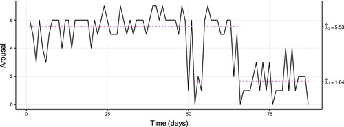
We estimated Poisson HMMs with varying number of states by nlminb with TMB's gradient and Hessian functions passed as arguments (this approach was chosen for all estimated models in our examples). The preferred HMM in terms of AIC and BIC is a two-state model, see Table A1 in Appendix 4.

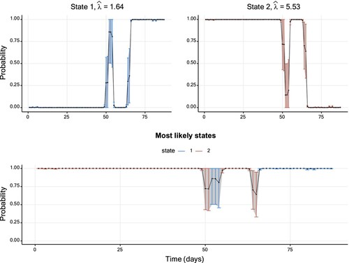
Figure 2 displays the corresponding smoothing probabilities with 95% Wald-type CIs, constructed using the standard error provided by TMB. Intuitively, one might expect the uncertainty to be low when a smoothing probability takes values close to zero or one, whereas higher uncertainty should be inherent to smoothing probabilities further away from these bounds. The CIs illustrated in Figure 2 follow this pattern. However, as pointed out by Bacri et al. [26], this data set is atypically short for fitting HMMs. As we will see in the following, different patterns will emerge for longer sequences of observations.

Figure 2. Smoothing probabilities and confidence intervals of a two-state Poisson HMM fitted to the TYT data set. The solid line shows the smoothing probability estimates and the 95% CIs are represented by vertical lines. The lower graph displays smoothing probabilities for the most likely state estimated for each data point. The vertical confidence interval lines are coloured differently per hidden state. Further details on parameter estimates are available in Table A1.

3.2. Soap

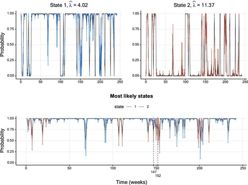
In the following, we consider a data set of weekly sales of a soap in a supermarket. The data were provided by the Kilts Center for Marketing, Graduate School of Business of the University of Chicago and are available in the database at https://research.chicagobooth.edu/kilts/marketing-databases/dominicks. The data are displayed in Figure 3. Similarly to the previous section, we fitted multiple Poisson HMMs, and the preferred HMM in terms of AIC and BIC is a two-state model as well (see Table A1 in Appendix 4). Figure 4 displays the smoothing probabilities resulting from this model. The patterns of the CIs described in the previous section are, in principle, also present here. Nevertheless, an exception is highlighted in the bottom panel of Figure 4: at t = 152, the smoothing probability of State 2 is closer to the upper boundary of one than the corresponding probability at t = 147. Yet, the uncertainty is higher at t = 152.

Figure 3. Plot of the soap data (of size 242), with a fitted two-state Poisson HMM. The coloured dots correspond to the conditional mean of the inferred state at each time. Table A1 displays the corresponding parameter estimates.

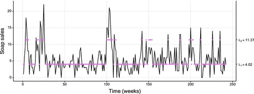
Figure 4. Smoothing probabilities and confidence intervals of a two-state Poisson HMM fitted to the soap data set. The solid line shows the smoothing probability estimates and the 95% CIs are represented by vertical lines. The lower graph displays smoothing probabilities for the most likely state estimated for each data point. The vertical confidence interval lines are coloured differently per hidden state. Further details on the parameter estimates are available in Table A1.

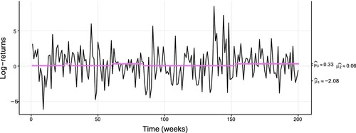
3.3. Weekly returns

The data set considered in this section are 2230 weekly log-returns based on the adjusted closing share price of the S&P 500 stock market index retrieved from Yahoo Finance, between January 1st 1980 and September 30th 2022. The returns are expressed in per cent to facilitate reading and interpreting the estimates. As shown, e.g. by Rydén et al. [45], Gaussian HMMs reproduce well certain stylized facts of financial returns. We thus estimated such models with varying number of states. A three-state model is preferred by the BIC, whereas the AIC is almost identical for three and four states (see Table A1 in Appendix 4). The estimates show a decrease in conditional standard deviation with increasing conditional mean. This is a well-known property of many financial returns (see, e.g.[46–48]) related to the behaviour of market participants in crisis and calm periods. Figure 5 shows the first 200 data points plotted along with conditional means from the preferred model.

Figure 5. Plot of the weekly returns data (of size 2230), with a fitted three-state Gaussian HMM. The coloured dots correspond to the conditional mean of the inferred state at each time, with a fitted three-state Gaussian HMM. Table A1 displays the corresponding parameter estimates. For readability, only the first 200 data are plotted.

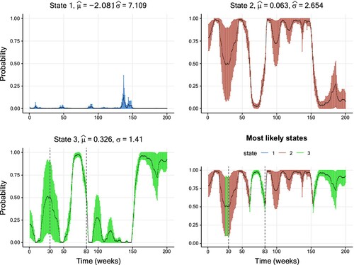
The subsequent Figure 6 shows inferred smoothing probabilities together with their CIs. In addition to the previous applications, where smoothing probabilities close to the boundary seemed to be linked to lower uncertainty, this data set shows also some clear exceptions from this pattern. For example, the smoothing probabilities of State 3 inferred at t = 30 and t = 83 take the relatively close values 0.51 and 0.53, respectively. However, the associated uncertainty at $t=30$ is visibly higher than the corresponding uncertainty at t = 83 (the estimated standard errors are 0.205 and 0.045). This may be explained by the fact that the inferred states closely around t = 30 oscillated between State 2 and 3, thus indicating a high uncertainty of the state classification during this period. On the contrary, around t = 83 a quick and persistent change from State 2 to 3 takes place.

Figure 6. Smoothing probabilities and confidence intervals of a three-state Gaussian HMM fitted to the weekly returns data set. The solid line shows the smoothing probability estimates and the 95% CIs are represented by vertical lines. The lower-right graph displays smoothing probabilities for the most likely state estimated for each data point. The vertical confidence interval lines are coloured differently per hidden state. For readability, only the first 200 out of the 2230 values are shown for readability purposes. Further details on the parameter estimates are available in Table A1.

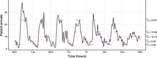
3.4. Hospital

Basis for our last example is a data set issued by the hospital ‘Hôpital Lariboisière’ from Assistance Publique – Hôpitaux de Paris (a french hospital trust). This data set consists of the hourly number of patient arrivals to the emergency ward during a period of roughly 10 years. A subset of the data (over one week) is displayed in Figure 7. We examine this due to several reasons. First, with 87648 observations, this data set is much larger than the ones examined previously. Secondly, the medical staff noticed differences between the rates of patient arrivals at day and night, respectively, which motivates the use of, e.g. an HMM. Last, a Poisson HMM is a natural candidate for the observed count-type data. The preferred model by both AIC and BIC has five states (see Table A2 in Appendix 4) and confirms the impression of the hospital employees: State 5 is mainly visited during core operating hours during day time. The fourth and third states mainly occur late afternoon, early evening, and early morning. Last, State 1 and 2 correspond to night time observations.

Figure 7. Plot of the hospital data (of size 87,648), with a fitted five-state Poisson HMM. The coloured dots correspond to the conditional mean of the inferred state at each time. Table A2 displays the corresponding parameter estimates. For readability, only the first week starting on Monday (from Monday January 4th 2010 at 00:00 to Sunday January 10th 2010 at 23:59) is plotted instead of the entire 10 years.

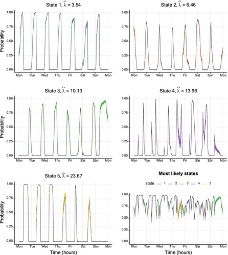
Even for a data set of this size, the smoothing probabilities and corresponding CIs can be derived with moderate computational effort and time: Figure 8 displays the results. Overall, the inferred CIs are relatively small, in particular in comparison with those obtained for the stock return data discussed in the previous example. The low uncertainty in the state classification may most likely result from the clear, close to periodic transition patterns.

Figure 8. Smoothing probabilities and confidence intervals of a five-state Poisson HMM fitted to the hospital data set. The solid line shows the smoothing probability estimates and the 95% CIs are represented by vertical lines. The lower-right graph displays smoothing probabilities for the most likely state estimated for each data point. The vertical confidence interval lines are coloured differently per hidden state. For readability, only the first week starting on Monday (from Monday January 4th 2010 at 00:00 to Sunday January 10th 2010 at 23:59) is plotted instead of the entire 10 years. Further details on the parameter estimates are available in Table A2.

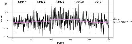
3.5. Simulated data

In contrast to the previous examples, we consider two simulated settings with data sets consisting of 500 observations each in this section. For both data sets, the underlying Gaussian HMM possesses three states with conditional mean vector $\mathit{\mu }=(-2,0,2)$. The difference lies in the conditional standard deviations. These equal $\mathit{\sigma }=(1,3,5)$ and $\mathit{\sigma }=(5,6.5,8)$ for the first and second data set, respectively. Thus, the two settings differ substantially w.r.t. the overlap of their conditional distributions. To facilitate comparability, we did not simulate state sequences from a pre-defined TPM, but generated identical state sequences in each setting: the states are visited in the order 1-2-3-2-1 with sojourns of length 100 in each state. Figures 9 and 10 show the observations along with the true sequence of states and their inferred conditional means for the setting with low and high overlap, respectively. Noteworthy is that ${\hat{\mu }}_3$ deviates quite a bit from the true value in the setting with high overlap. This may most likely result from the high conditional variance in the third state.

Figure 9. Plot of the first simulated data set (of size 500) with low overlap, with a fitted three-state Gaussian HMM. The vertical dotted lines separate the true states of the data indicated by text, and the coloured dots correspond to the conditional mean of the inferred state at each time. Table A3 displays the corresponding parameter estimates.

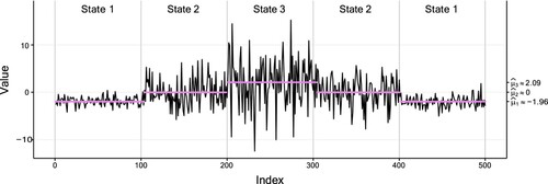
Figure 10. Plot of the second simulated data set (of size 500) with high overlap, with a fitted three-state Gaussian HMM. The vertical dotted lines separate the true states of the data indicated by text, and the coloured dots correspond to the conditional mean of the inferred state at each time. Table A3 displays the corresponding parameter estimates.

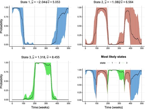
Furthermore, Figure 11 displays the inferred smoothing probabilities together with their CIs for the first setting. For these well-separated conditional distributions, the inferred state sequence is in high accordance with the true states. Furthermore, the width of the CIs is generally low with a slight increase around periods of state changes. In contrast, Figure 12 corresponding to the second setting with high overlap paints a different picture. First, the width of the CIs is substantially higher than in the first setting. Secondly, the inferred state sequence partly deviates substantially from the true state sequence, in particular from t = 300 until approximately t = 350. During this period, the inferred state sequence remains in State 3, although state change to the second state has already happened. Along with this misclassification come comparably wide CIs, considering that the smoothing probabilities take values mostly above 90%.

Figure 11. Smoothing probabilities and confidence intervals of a three-state Gaussian HMM fitted to the first simulated data set with low overlap. The solid line shows the smoothing probability estimates and the 95% CIs are represented by vertical lines. The lower-right graph displays smoothing probabilities for the most likely state estimated for each data point. The vertical confidence interval lines are coloured differently per hidden state. Further details on the parameter estimates are available in Table A3.

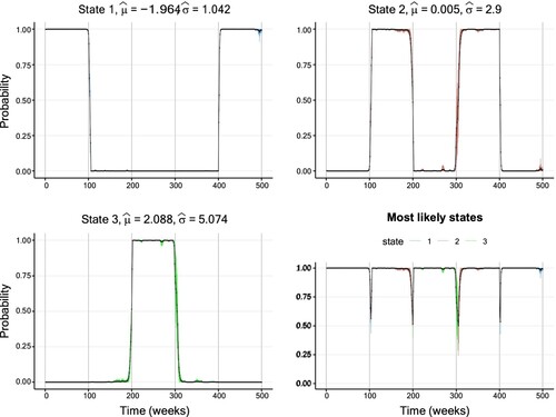
Figure 12. Smoothing probabilities and confidence intervals of a three-state Gaussian HMM fitted to the second simulated data set with high overlap. The solid line shows the smoothing probability estimates and the 95% CIs are represented by vertical lines. The lower-right graph displays smoothing probabilities for the most likely state estimated for each data point. The vertical confidence interval lines are coloured differently per hidden state. Further details on the parameter estimates are available in Table A3.

4. Performance and accuracy of different optimizers

This section compares the speed and accuracy of different optimizers in R using TMB in an HMM estimation setting with DNM by several simulation studies with different settings.

In the first setting, we simulate time series consisting of 87 observations from a two-state Poisson HMM fitted to the TYT data, as we want to examine the different optimizers performance on data sets with relatively few observations. In the second setting, we simulate time series of length 200 from a two-state Poisson HMM, and in the third setting, time series of length 200 from a two-state Gaussian HMM are simulated. The specific choice of parameters is described in more detail in the forthcoming sections.

The comparisons that focus on computational speed and iterations of the different optimizers, are based on 200 replications from the different models, while the studies focusing on the accuracy of the optimizers are based on 1000 replications from the different models. Hence, the Monte-Carlo simulation setup in this paper closely resembles the setup of [26].

4.1. Computational setup

The results presented in this paper required installing and using the R-package TMB and the software Rtools, where the latter is needed to compile C++ code. Scripts were coded in the interpreted programming language R [49] using its eponymous software environment RStudio. For the purpose of making our results reproducible, the generation of random numbers is handled with the function set.seed under R version number 3.6.0. A seed is set multiple times in our scripts, ensuring that smaller parts can be easily duplicated without executing lengthy prior code. A workstation with 4 Intel(R) Xeon(R) Gold 6134 processors (3.7 GHz) running under the Linux distribution Ubuntu 18.04.6 LTS (Bionic Beaver) with 384 GB RAM was used to execute our scripts.

4.2. Selected optimizers and additional study design

There exist a large number of optimizers for use within the R ecosystem, see e.g. [50]. In a preliminary phase, multiple optimization routines were attempted, and the ones failing to converge on a few selected test data sets from the designs mentioned above were excluded (details available from the author upon request). Hence, the following optimizers were selected for the simulation studies:

• optim from the stats package to test the BFGS [51–54], L-BFGS-B [55], CG [56], and Nelder–Mead [32] algorithms.

• nlm [57] and nlminb [27] from the same package to test popular nonlinear unconstrained optimization algorithms.

• hjn from the optimr package [28] to test the so-called Hooke and Jeeves Pattern Search Optimization [58].

• marqLevAlg from the marqLevAlg package [59] to test a general-purpose optimization based on the Marquardt-Levenberg algorithm [60,61].

• BBoptim from the BB package [62] to test a spectral projected gradient method for large scale optimization with simple constraints [63].

• newuoa from the minqa package [64] to test a large-scale nonlinear optimization algorithm [65].

By also providing the Hessian and/or gradient to the optimizers that support such inputs, 22 optimization procedures are examined for each study design. For the study of the computational speed and number of iterations, we applied the microbenchmark package [66] that allows us to obtain precise durations for each of the simulated data sets. Furthermore, HMM ML estimates were reordered by increasing Poisson rates or Gaussian means to avoid a random order of the states.

It is important to note that we discarded all those samples for which the simulated state sequence did not sojourn at least once in each state. This was to avoid identifiability and convergence issues when trying to estimate a m-state HMM on a data set where only m−1 states are visited. Further, samples where at least one optimizer failed to converge were also discarded to ensure comparability. For the same reason, we set the maximum number of iterations to ${10}^4$ whenever possible. Note that some optimizers (BFGS, CG, hjn, L-BFGS-B, Nelder-Mead, newuoa) do not report a number of iterations and are therefore missing from our comparisons of iterations. Finally, we use the true values as initial parameters. For the TYT data, initial values are calculated as medians from the fitted models resulting from all optimizers listed above.

4.3. Results

In this section, we report the results from the simulation studies focusing on the performance of different optimizers in terms of the computational speed and the lack or presence of unreasonable estimates. This section uses R scripts that may be of interest to users investigating their own HMM settings, and are available in the supporting information. We begin by reporting the speed of all optimization routines and thereafter the accuracy. The routine names contain the optimizer names and may be followed by either ‘_gr’ to indicate that the routine uses TMB's provided gradient function, ‘_he’ to indicate the use of TMB's provided Hessian function, or ‘_grhe’ to indicate the use of both gradient and Hessian functions provided by TMB. Note that some optimizers cannot make use of these functions and hence bear no extension at the end of their names.

4.3.1. Simulation study: TYT setting

Figure 13 shows the time required by each optimization routine, measured over the 200 replication. The number of iterations required by each optimization routine is also reported where available. Times range from 1 to 1340 milliseconds. As shown by the large medians and wide CIs, CG and CG_gr require substantially more time to estimate an HMM, compared to the other optimizers. Furthermore, optimizers that take a long time to estimate HMMs require a high amount of iterations as well, as expected. Notably, optimization routines almost always take longer when the Hessian is passed. This likely results from a higher computational burden due to handling and evaluating Hessian matrices via TMB.

Figure 13. Median number of iterations and median duration (in milliseconds and ranked) together with 2.5%- and 97.5%-quantile when fitting two-state Poisson HMMs to 200 replications in the first setting. The horizontal axes are on a logarithmic scale (base 10). More detailed values are available at Table A4.

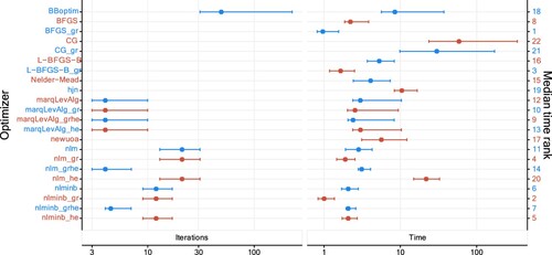
Figure 14. Median number of iterations and median duration (in milliseconds and ranked) together with 2.5%- and 97.5%-quantile when fitting two-state Poisson HMMs to 200 replications in the second setting. The horizontal axes are on a logarithmic scale (base 10). More detailed values are available at Table A5.

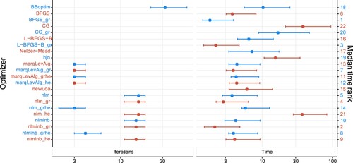
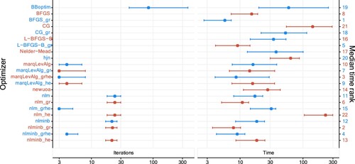
Figure 15. Median number of iterations and median duration (in milliseconds and ranked) together with 2.5%- and 97.5%-quantile when fitting two-state Gaussian HMMs to 200 replications in the third setting. The horizontal axes are on a logarithmic scale (base 10). More detailed values are available at Table A6.

Looking at the details, the optimizer BFGS_gr is among the fastest optimizers, and this is partly explained by a relatively low number of iterations, and by the fact that it does not make use of the Hessian. However, we note that nlm and nlmimb families of optimizers are slower when the gradient and Hessian are not passed as argument. The optimizer BBoptim is comparatively slow, and nlminb_grhe fails to converge comparably often.

In addition to time durations, we investigate the accuracy of the optimizers, based on another 1000 replications from the two-state Poisson HMM in the first setting. The main conclusion from this simulation is that the medians and empirical quantiles calculated are in fact almost identical across all optimizers, and very close to the true parameter values used in the simulations. Results are reported in Figure A1 in Appendix 5. These result imply that the different optimizers are equally accurate. Note, however, that the variation is quite high for some of the estimated parameters and for the nll, which results most likely from the limited number of observations.

4.3.2. Simulation study: two-state Poisson HMM

In this second simulation setting, the parameters of our two-state Poisson HMM are given by $\mathit{\lambda }=(1,7),\mathbf{\Gamma }=\left(\begin{array}{cc}0.95& 0.05\\ 0.15& 0.85\end{array}\right),$and the sample size is fixed at 200. Figure 14 illustrates our results, which are in line with those obtained in the first setting. More precisely, BBoptim still dominates the number of iterations, and CG and CG_gr require more computational time than the others. Overall, most optimizers need more time compared to the previous setting as there is more data to process, but the time increase for nlm_he and hjn is much more substantial than for other optimizers. Moreover, although the data set is larger, some optimizers (e.g. BBoptim and BFGS_gr) perform as fast as or faster than in the previous setting. Furthermore, passing TMB's Hessian to optimizers does not always slow down the optimization. This can be seen, e.g. from nlminb_he which exhibits a lower median time than nlminb. A last notable pattern concerns the popular nlm optimizer. When only the Hessian but not the gradient is supplied from TMB, the computational time increases substantially compared to nlm_gr and nlm_grhe. Interestingly, the equally popular optimizer nlminb is not affected in the same way. Thus, one should be careful when only supplying the Hessian from TMB while an optimizer carries out the gradient approximation. In any case, the low number of iterations required by both nlminb_grhe and nlm_grhe indicate a preferable convergence behaviour when supplying both quantities.

In terms of accuracy of the parameter estimates and obtained nlls, our results are highly similar to those described in the first setting (for details, see Figure A2 in Appendix 5).

4.3.3. Simulation study: two-state Gaussian HMM

In our third and last simulation setting, the parameters of a two-state Gaussian HMM are given by $\mathbf{\Gamma }=\left(\begin{array}{cc}0.95& 0.05\\ 0.15& 0.85\end{array}\right),\mathit{\mu }=(-5,5),\mathit{\sigma }=(1,5),$and the sample size is fixed at 200. In terms of computational time and the number of iterations, the results observed for this setup are similar to the previously studied Poisson HMMs (see Figure 15). A minor aspect is an increase in both iterations and computational time, which is not surprising given the higher number of parameters.

Regarding estimation accuracy of the parameter estimates and obtained nlls, our results are again highly similar to those obtained in the previous two settings (illustrated graphically by Figure A3 in Appendix 5).

5. Robustness to initial value selection

In this section, we examine the impact of initial values of the parameters – including poorly selected ones – on the convergence behaviour and accuracy of different optimizers. We investigate one real and several simulated data sets. In order to ‘challenge’ the optimizers, all data sets are of comparable small size.

5.1. Study design

We again consider three settings in the following. In the first, we investigate the TYT data set. In the second and third setting, we focus on simulated data from Poisson and Gaussian HMMs, respectively. More specifically, for the Poisson HMMs we generate one data set of sample size 200 for each of the HMMs considered. These HMMs are defined by all possible combinations of the following Poisson rates and TPMs: $\begin{array}{rl}& \mathit{\lambda }\in \{(1,4),(5,7)\}\mathrm{and}\\ & \mathbf{\Gamma }\in \{\left(\begin{array}{cc}0.9& 0.1\\ 0.2& 0.8\end{array}\right),\left(\begin{array}{cc}0.7& 0.3\\ 0.8& 0.2\end{array}\right),\left(\begin{array}{cc}0.1& 0.9\\ 0.8& 0.2\end{array}\right),\left(\begin{array}{cc}0.55& 0.45\\ 0.45& 0.55\end{array}\right)\}.\end{array}$This setup leads to the generation of $2\times 4$ data sets. For the Gaussian HMMs, we follow the same approach, where the Gaussian means and standard deviations are selected from the sets $\begin{array}{rl}\mathit{\mu }& \in \{(-2,2),(-1,4)\}\mathrm{and}\\ \mathit{\sigma }& \in \{(1.5,2.5),(0.5,1.5)\}.\end{array}$This setting thus generates $2\times 2\times 4$ data sets.

For each data set, we pass a large range of initial values to the same optimizers considered in the previous section. In this way, we investigate the resistance of each optimizer to potentially poor initial values when fitting HMMs. To generate sets of initial values, we consider the following potential candidates for Poisson rates $\mathit{\lambda }$, Gaussian means $\mathit{\mu }$, Gaussian standard deviations $\mathit{\sigma }$, and TPMs $\mathbf{\Gamma }$: $\begin{array}{rl}{\lambda }_1,{\lambda }_2& \in \{M,M+0.5,M+1,1.5,\dots ,x_{max}\},\text{where }{\lambda }_1<{\lambda }_2,\\ {\mu }_1,{\mu }_2& \in \{x_{min},x_{min}+0.5,x_{min}+1,\dots ,x_{max}-0.5,x_{max}\},\text{ where }{\mu }_1<{\mu }_2,\\ {\sigma }_1,{\sigma }_2& \in \{10\text{ equidistant points going from }\sqrt{\frac{(x_{max}-x_{min}{)}^2}{2T}}\text{ to }\\ & \sqrt{(x_{max}-\hat{\mu })(\hat{\mu }-x_{min})}\phantom{\sqrt{\frac{(x_{max}-x_{min}{)}^2}{2T}}}\},\\ \text{ and}\mathbf{\Gamma }& \in \{\left(\begin{array}{cc}0.1& 0.9\\ 0.9& 0.1\end{array}\right),\left(\begin{array}{cc}0.1& 0.9\\ 0.8& 0.2\end{array}\right),\dots ,\left(\begin{array}{cc}0.1& 0.9\\ 0.1& 0.9\end{array}\right),\\ & \left(\begin{array}{cc}0.2& 0.8\\ 0.9& 0.1\end{array}\right),\left(\begin{array}{cc}0.2& 0.8\\ 0.8& 0.2\end{array}\right),\dots ,\left(\begin{array}{cc}0.2& 0.8\\ 0.1& 0.9\end{array}\right),\\ & ,\dots \left(\begin{array}{cc}0.9& 0.1\\ 0.1& 0.9\end{array}\right)\},\end{array}$where $x_{min}=min(x_1,x_2,\dots ,x_T)$, $x_{max}=max(x_1,x_2,\dots ,x_T)$, $\hat{\mu }=\frac{1}{T}$ $\sum _{i=1}^T{x}_i$ and $M=max(0.5,x_{min})$. The motivation for this selection is as follows. First, Poisson means have to be greater than zero, so we set their lower boundary to M. Secondly, the ${\hat{\lambda }}_i$'s have to belong to the interval $(x_{min},x_{max})$, cfr. [67]. This applies to the Gaussian means as well. Thirdly, the upper and lower limit of ${\sigma }_1,{\sigma }_2$ is motivated by the Bhatia-Davis [68] and the von Szokefalvi Nagy inequalities [69].

For the Poisson HMMs fitted, we consider all possible combination of the parameters described above. For the Gaussian HMMs, however, we sample 12,500 initial parameters for each of the 16 data sets to reduce computation time (the total amount reduces from 39,066,300 to 200,000). These sets of initial values are identical for all optimizers. As in the previous Section 4, we limit the maximal number of iterations to ${10}^4$ whenever possible. Other settings were left as default.

To evaluate the performance of the optimizers considered, we rely on two criteria. First, we register whether the optimizer converges (all errors are registered regardless of their type). Secondly, when an optimizer converges, we also register if the nll is equal to the ‘true’ nll (with a gentle margin of ± 5%). We calculate this ‘true’ nll as the median of all nlls derived with all optimizers initiated with the true parameter values.

5.2. Results

Table 1 shows the results for the two-state Poisson HMMs fitted to the TYT data. The four marqLevAlg follow closely. We note that hjn has the best performance: it basically does not fail and converges almost always. Moreover, nlminb_grhe fails to converge much more often than other optimizers, but is the most likely to find the global maximum when it converges. For the other optimizers, the failure rate is generally low (less than 5%) and the global maximum is found in more than 65% of the cases.

Table 1. Performance of multiple optimizers estimating Poisson HMMs from the TYT data (first setting) over 7371 different sets of initial parameters.

	Failures $(\mathrm{\%})$	Global maximum found $(\mathrm{\%})$
BBoptim	0.00	72.11
BFGS	0.00	66.83
BFGS_gr	0.00	66.83
CG	4.90	71.48
CG_gr	4.91	71.49
hjn	0.00	97.40
L-BFGS-B	3.43	71.38
L-BFGS-B_gr	3.46	71.22
marqLevAlg	1.64	88.43
marqLevAlg_gr	1.99	88.64
marqLevAlg_grhe	1.94	88.60
marqLevAlg_he	1.64	88.43
Nelder-Mead	0.00	69.88
newuoa	0.00	71.67
nlm	0.00	65.19
nlm_gr	0.00	65.22
nlm_grhe	0.00	72.99
nlm_he	0.00	65.19
nlminb	0.00	74.96
nlminb_gr	0.00	74.94
nlminb_grhe	24.41	99.96
nlminb_he	0.00	74.96

Notes: The first column lists all optimizers. The second column shows how often optimizers fail to converge successfully. The third column displays how often optimizers successfully found the global maximum of the nll when converging.

Table 2 reports the results from the second setting, also with two-state Poisson HMMs. The results show that all optimizers find the global maximum in the majority of cases($>96\mathrm{\%}$) when converging. Moreover, the failure rates are relatively low for all optimizers with the exception of CG, which stands out with comparably high failure rates.

Table 2. Performance of multiple optimizers estimating Poisson HMMs from the second setting over 194,481 different sets of initial parameters.

	Failures $(\mathrm{\%})$	Global maximum found $(\mathrm{\%})$
BBoptim	4.20	100.00
BFGS	0.00	96.68
BFGS_gr	0.00	96.68
CG	14.23	99.49
CG_gr	14.47	99.53
hjn	0.00	99.99
L-BFGS-B	0.30	100.00
L-BFGS-B_gr	0.29	100.00
marqLevAlg	3.19	99.98
marqLevAlg_gr	3.20	100.00
marqLevAlg_grhe	3.20	100.00
marqLevAlg_he	3.19	99.98
Nelder-Mead	0.00	99.91
newuoa	0.34	99.77
nlm	0.07	98.42
nlm_gr	0.02	98.42
nlm_grhe	0.00	99.50
nlm_he	0.07	98.42
nlminb	0.00	100.00
nlminb_gr	0.00	100.00
nlminb_grhe	4.62	100.00
nlminb_he	0.00	100.00

Notes: The first column lists all optimizers. The second column shows how often optimizers fail to converge successfully. The third column displays how often optimizers successfully found the global maximum of the nll when converging.

Finally, Table 3 presents the results from the third setting with Gaussian HMMs. The results regarding the failure rates point in the same direction as those from the Poisson HMM setting: CG attains the highes failure rate, followed by newuoa and L-BFGS-B. The remaining optimizers perform satisfactorily. Note, however, that nlminb does not benefit from being supplied with the gradient and Hessian from TMB. Regarding the global maximum found, many algorithms reach success rates of about 95% or more. Notable exceptions are Nelder-Mead and nlm when not both gradient and Hessian are provided by TMB. As observed previously for the TYT data, nlm benefits strongly from the full use of TMB.

Table 3. Performance of multiple optimizers estimating Gaussian HMMs from the third setting over 200,000 different sets of initial parameters randomly drawn from 39,066,300 different candidate sets of initial values.

	Failures $(\mathrm{\%})$	Global maximum found $(\mathrm{\%})$
BBoptim	1.13	98.61
BFGS	0.00	84.24
BFGS_gr	0.00	84.24
CG	8.62	98.68
CG_gr	8.82	98.81
hjn	0.53	95.21
L-BFGS-B	6.58	94.40
L-BFGS-B_gr	6.75	94.45
marqLevAlg	2.55	98.18
marqLevAlg_gr	2.66	98.34
marqLevAlg_grhe	2.64	98.33
marqLevAlg_he	2.55	98.18
Nelder-Mead	0.03	80.55
newuoa	7.58	97.44
nlm	0.39	87.77
nlm_gr	0.11	87.73
nlm_grhe	0.32	97.21
nlm_he	0.39	87.77
nlminb	0.22	97.18
nlminb_gr	0.26	97.20
nlminb_grhe	5.69	97.97
nlminb_he	0.22	97.18

Notes: The first column lists all optimizers. The second column shows how often optimizers fail to converge successfully. The third column displays how often optimizers successfully found the global maximum of the nll when converging.

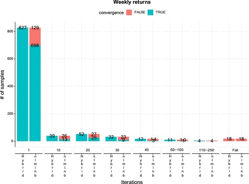
Figure 16. Convergence counts of nlminb and a hybrid algorithm (first Nelder-Mead, then nlminb). The hybrid algorithm uses $1,10,20,\dots$ iterations for the Nelder-Mead, then passes the estimates to nlminb as initial values. We randomly picked 1000 sets of initial values out of 1,458,000 potential candidates.

5.3. Hybrid algorithm

Last, we ran a small simulation study investigating a hybrid algorithm within the TMB framework in the spirit of [29]. The hybrid algorithm starts with the Nelder-Mead optimizer and switches to nlminb after a certain number of iterations. The idea is to benefit from both Nelder-Mead's rapid departure from poor initial values and from the high convergence speed of nlminb. Our study is performed on 1000 random sets of initial values in a similar fashion to Section 5, using the weekly returns data set. For every set of initial values, we sequentially increase the number of iterations carried out by Nelder-Mead by ten (starting at one) until convergence or until 10,000 iterations has been reached, in which case we classify the attempt as a failure. For comparison, we also run an optimization only with nlminb starting directly with the same sets of inital values. In both cases, nlminb benefits from the gradient and Hessian provided by TMB.

Figure 16 reports the results of our study. The left most columns show that only one iteration was required to converge in 827 of the 1000 sets of initial values with the hybrid algorithm, while nlminb converges in only 698 out of these 827 sets. Furthermore, for 39 additional sets of initial values, the hybrid algorithm converges with 10 iterations carried out by the Nelder-Mead optimizer, whereas nlminb fails 26 times on these sets. Increasing the number of initial iterations carried out by Nelder-Mead for the hybrid algorithm leads to similar patterns. Finally, both optimization routines fail to converge for 18 sets of initial values. Thus, in total, the hybrid algorithm with one or more Nelder-Mead iterations failed in only $1.8\mathrm{\%}$ of the cases. In comparison, direct use of nlminb failed in around $12\mathrm{\%}$ of the cases. This indicates that the hybrid algorithm requires rather few iterations of Nelder-Mead to improve the convergence rate substantially.

6. Concluding remarks

This paper addresses a couple of aspects concerning parameter estimation for HMMs via TMB and R using direct numerical maximization (DNM) of the likelihood. The advantage of TMB is that it permits to quantify the uncertainty of any quantity depending on the estimated parameters. This is achieved by combining the delta method with automatic differentiation. Moreover, TMB provides exact calculations of first- and second-order derivatives of the (log-)likelihood of a model by automatic differentiation. This allows for efficient gradient- and/or Hessian-based optimization of the likelihood. In the first part of the paper, we propose a straightforward technique to quantify the uncertainty of smoothing probabilities via the calculation of Wald-type CIs. The advantage of this approach is that one avoids computationally intensive bootstrap methods. By means of several examples, we illustrate how such CIs provide additional insight into the commonly used state classification via smoothing probabilities. For a practitioner working with HMMs, the presented uncertainty quantification constitutes a new tool for obtaining a better understanding of the dynamics of the hidden process.

Subsequently, we examine speed and accuracy of the different optimizers in three simulation settings. Our results show a slight variation in both number of iterations and computational speed. In particular, the optimizers nlminb, nlm, marqLevAlg, and BFGS usually possess the highest computational speed. The computing time required by all optimizers reduces when using the gradient provided by TMB. The number of iterations reduces in particular for nlminb and nlm when employing both gradient and Hessian from TMB. This suggests a more direct path towards the (global) likelihood maximum compared to optimizer-internal approximation routines. Regarding the accuracy, measured in terms of attained negative log-likelihood and parameter estimates (and their variability) the results show little variations across the different optimizers. This is indeed a positive finding, indicating that the performance of the optimizers is relatively equal in terms of accuracy – however, this statement only holds true when using the optimal initial value. Then, we examine robustness towards initial values across different optimizers. In three settings, we measure (a) how often optimizers fail to converge and (b) how often they successfully reach the global maximum of the log-likelihood function when starting from a wide range of sets of initial values. In particular, nlm, nlminb, and hjn show an overall good performance. Notably, nlm benefits strongly from employing both gradient and Hessian provided by TMB, which is not the case for nlminb. Altogether, we observe a trade-off between failure rates and convergence to the global maximum. Nevertheless, none of the optimizers shows an exceptionally bad performance.

Finally, we illustrate that a hybrid algorithm starting with the Nelder-Mead optimizer and switching to nlminb after a certain number of iterations converges more often than nlminb. Notably an effect is visible even with a single initial iteration carried out by Nelder-Mead.

Concerning future research, initialization strategies and the hybrid algorithm may merit further investigation. While our hybrid strategy is implemented easily and seems effective, initial values considered are based on a simple random sampling process. More complex approaches could be considered in case of unsatisfactory performance, which may be expected, e.g. for models with a high number of parameters or high-dimensional data. Then one may consider EM short-runs, (model-based) clustering, or other alternatives [see 29, 38, and the references therein] – potentially at the expense of increased mathematical and programming efforts. In our results concerning different optimization algorithms in the context of TMB provide useful guidance when pre-selecting suitable candidates for further analyses. Furthermore, smoothing probabilities play a key role for the model selection criterion ICL [70] through their contribution to the entropy term (roughly speaking,ICL = BIC – $2\cdot$ Entropy). Hence, it may be possible to develop a model selection criterion which additionally takes the uncertainty of the smoothing probabilities into account. The increasing width of the CIs during periods of wrongful state classification could serve as additional input for model selection on the one hand. On the other hand, it could constitute itself an interesting measure for identifying misclassification.

Acknowledgments

We thank the University of Regensburg and European School for Interdisciplinary Tinnitus Research (ESIT) for providing access to the TYT data. Special thanks go to J. Simões for data preparation, and W. Schlee and B. Langguth for helpful comments and suggestions. We also thank Anthony Chauvin and Bertrand Galichon for providing access to the hospital data set along with the necessary authorizations. Furthermore, our thanks go to an anonymous reviewer, who provided very valuable feedback and criticism. Many thanks go to Hans Karlsen for his valuable help. Last, J. Bulla's profound thanks for the continued moral support go to the highly skilled, very helpful, and always friendly employees of Vestbrygg AS (Org. ID 912105954).

Disclosure statement

No potential conflict of interest was reported by the author(s).

Additional information

Funding

The work of J. Bulla was supported by the GENDER NET Plus Grant agreement ID: 741874. DOI: 10.3030/741874 [GNP-182]. This work was also supported by the Financial Market Fund [Norwegian Research Council project no. 309218].

Appendices

Appendix 1.

Forward algorithm and backward algorithm

The pass through observations can be efficiently computed piece by piece, from left (i.e. time s = 1) to right (i.e. time s = t) or right to left by the so-called ‘forward algorithm’ and ‘backward algorithm’ respectively. With these two algorithms, the likelihood can be computed recursively. To formulate the forward algorithm, let us define the vector ${\alpha }_t$ for $t=1,2,\dots ,T$ so that $\begin{array}{rl}{\mathit{\alpha }}_t& =\mathit{\delta }\mathit{P}(x_1)\mathbf{\Gamma }\mathit{P}(x_2)\mathbf{\Gamma }\mathit{P}(x_3)\dots \mathbf{\Gamma }\mathit{P}(x_t)\\ & =\mathit{\delta }\mathit{P}(x_1)\prod _{s=2}^t\mathbf{\Gamma }\mathit{P}(x_s)\\ & =({\alpha }_t(1),\dots ,{\alpha }_t(m))\end{array}$for $t=1,2,\dots ,T$. The name of the algorithm comes from computing it via the recursion $\begin{array}{rl}{\mathit{\alpha }}_0& =\mathit{\delta }\mathit{P}(x_1),\\ {\mathit{\alpha }}_t& ={\mathit{\alpha }}_{t-1}\mathbf{\Gamma }\mathit{P}(x_t)\text{ for }t=1,2,\dots ,T.\end{array}$After passing through all observations until time T, the likelihood is derived from $L(\mathit{\theta })={\mathit{\alpha }}_T{\mathbf{1}}^{\prime }.$The backward algorithm is very similar to the forward algorithm. The sole difference lies in starting from the last instead of the first observation. To specify the backward algorithm, let us define the vector ${\mathit{\beta }}_t$ for $t=1,2,\dots ,T$ so that $\begin{array}{rl}{\mathit{\beta }}_t^{\prime }& =\mathbf{\Gamma }\mathit{P}(x_{t+1})\mathbf{\Gamma }\mathit{P}(x_{t+2})\dots \mathbf{\Gamma }\mathit{P}(x_T)\dots {\mathbf{1}}^{\prime }\\ & =(\prod _{s=t+1}^T\mathbf{\Gamma }\mathit{P}(x_s)){\mathbf{1}}^{\prime }\\ & =({\beta }_t(1),\dots ,{\beta }_t(m)).\end{array}$The name backward algorithm results from the way of recursively calculating ${\mathit{\beta }}_t$ by $\begin{array}{rl}{\mathit{\beta }}_T& ={\mathbf{1}}^{\prime }\\ {\mathit{\beta }}_t& =\mathbf{\Gamma }\mathit{P}(x_{t+1}){\mathit{\beta }}_{t+1}\text{ for}t=T-1,T-2,\dots ,1.\end{array}$As before, the likelihood can be obtained after a pass through all observations by $L(\mathit{\theta })=\mathit{\delta }{\mathit{\beta }}_1.$Usually, only the forward algorithm is used for parameter estimation. Nonetheless, either or both algorithms may be necessary to derive certain quantities of interest, e.g. smoothing probabilities (as we explore in Section 3) or forecast probabilities. For practical implementation, attention needs to be paid to underflow errors which can quickly occur in both algorithms (due to the elements of the TPM and / or conditional probabilties taking values in $[0,1]$). Therefore, we implemented a scaled version of the forward algorithm as suggested by Zucchini et al. [22, p. 48]. This version directly provides the negative log-likelihood (nll) as result.

Appendix 2.

Reparameterization of the likelihood function

Along with the data, $\mathit{\theta }$ serves as input for calculating the likelihood by the previously illustrated forward algorithms. Some constraints need to be imposed on $\mathit{\theta }$:

1. In the case of the Poisson HMM, the parameter vector $\mathit{\lambda }=({\lambda }_1,\dots ,{\lambda }_m)$ necessary for computing the conditional distribution has to consist of strictly positive elements.

2. The elements ${\gamma }_{ij}$ of the TPM $\mathbf{\Gamma }$ must be non-negative, and each row of $\mathbf{\Gamma }$ needs to sum up to to one.

Tacking these constraints by means of constrained optimization routines when maximizing the likelihood can lead to several difficulties. For example, constrained optimization routines may require a significantly amount of fine-tuning. Moreover, the number of available optimization routines is significantly reduced. A common alternative works by reparametrizing the log-likelihood as a function of unconstrained, so-called ‘working’ parameters $\{\mathbf{T}\mathbf{,}\mathit{\eta }\}\mathbf{=}{\mathbf{g}}^{\mathbf{-}\mathbf{1}}\mathbf{(}\mathbf{\Gamma }\mathbf{,}\mathit{\lambda }\mathbf{)}$, as follows. One possibility to reparametrize $\mathbf{\Gamma }$ is given by ${\tau }_{ij}=\log \left(\frac{{\gamma }_{ij}}{1-\sum _{k\ne i}{\gamma }_{ik}}\right)=\log ({\gamma }_{ij}/{\gamma }_{ii})\text{ for}i\ne j.$where ${\tau }_{ij}\in \mathbb{R}$ are $m(m-1)$ unconstrained elements of an $m\times m$ matrix $\mathbf{T}$ with missing diagonal elements. The matching reverse transformation is ${\gamma }_{ij}=\frac{\exp ({\tau }_{ij})}{1+\sum _{k\ne i}\exp ({\tau }_{ik})}\text{ for}i\ne j,$and the diagonal elements of $\mathbf{\Gamma }$ follow from $\sum _j{\gamma }_{ij}=1$, $i=1,\dots ,m$ (see [22], p. 51).

For a Poisson HMM, a simple method to reparametrize the conditional Poisson means $\mathit{\lambda }$ into $\mathit{\eta }$ is given by ${\eta }_i=\log ({\lambda }_i)$ for $i=1,\dots ,m$. Consequently, the constrained ‘natural’ parameters are obtained via ${\lambda }_i=\exp ({\eta }_i)$. Estimation of the natural parameters $\{\mathbf{\Gamma },\mathit{\lambda }\}$ can therefore be obtained by maximization of the reparametrized likelihood with respect to $\{\mathbf{T}\mathbf{,}\mathit{\eta }\}$ then by a transformation of the estimated working parameters back to natural parameters via the above transformations, i.e. $\{\hat{\mathbf{\Gamma }},\hat{\mathit{\lambda }}\}=g(\hat{\mathit{T}},\hat{\mathit{\eta }})$. In general, the above procedure requires that the function g is one-to-one.

With a Gaussian HMM, the means are already unconstrained and do not require any transformation. However, the standard deviations can be transformed similarly to the Poisson rates via ${\eta }_i=\log ({\sigma }_i)$ for $i=1,\dots ,m$, and the ‘natural’ parameters are then obtained via the corresponding reverse transformation ${\sigma }_i=\exp ({\eta }_i)$.

Appendix 3.

Confidence intervals

When handling statistical models, confidence intervals (CIs) for the estimated parameters can be derived via various approaches. One common such approach bases on finite-difference approximations of the Hessian. However, as [71] points out, there are better alternatives when dealing with most HMMs. Preferred are profile likelihood-based CIs or bootstrap-based CIs, where the latter are now widely used despite the potentially large computational load [22,29]. With common Poisson HMMs, [26] shows that TMB can yield valid Wald-type CIs in a fraction of the time required by classical bootstrap-based methods.

In this section, we describe the Wald-type and the bootstrap-based approach. The likelihood profile method frequently fails to yield CIs (see [26]) and is therefore not detailed.

A.1. Wald-type confidence intervals

Evaluating the Hessian at the optimum found by numerical optimization procedures is basis for Wald-tye CIs. As illustrated above, the optimized negative log-likelihood function of a HMM typically depends on the working parameters. However, drawing inference on the natural parameters is by far more relevant than inference on the working parameters. To overcome this problem we can take advantage of the delta method [see, e.g. 72, 73]. For applying the delta method in general, let the d-dimensional vector $\hat{\mathit{\psi }}$ be an estimate of $\mathit{\psi }$ based on a sample of size n such that $\sqrt{n}(\hat{\mathit{\psi }}-\mathit{\psi })\stackrel{D}{\to }{\mathcal{N}}_d(0,\mathbf{\Sigma }),$where ${\mathcal{N}}_d(0,\mathbf{\Sigma })$ denotes the d-dimensional centred Normal distribution with covariance matrix $\mathbf{\Sigma }$, and $\stackrel{D}{\to }$ denotes convergence in distribution. Then, we have $\sqrt{n}(g(\hat{\mathit{\psi }})-g(\mathit{\psi }))\stackrel{D}{\to }{\mathcal{N}}_s(0,\mathrm{\nabla }g(\mathit{\psi })\cdot \mathbf{\Sigma }\cdot \mathrm{\nabla }g(\mathit{\psi }{)}^{\mathrm{\prime }})$for any function $g:{\mathbb{R}}^d\to {\mathbb{R}}^s$ with $\mathrm{\nabla }g(\mathit{\psi })$ denoting its Jacobian matrix.

In a general HMM setting, let $\mathit{\eta }$ represent working parameters with a one-to-one correspondence to a set of natural parameters $\mathit{\lambda }$ in an arbitrary conditional distribution. Since the Hessian ${\mathrm{\nabla }}^2\log L(\{\hat{\mathit{T}},\hat{\mathit{\eta }}\})$ relies on the working parameters $\{\hat{\mathit{T}},\hat{\mathit{\eta }}\}$, an estimate of the covariance matrix of $\{\hat{\mathbf{\Gamma }},\hat{\mathit{\lambda }}\}$ can therefore be obtained via the delta method through ${\mathrm{\Sigma }}_{\hat{\mathbf{\Gamma }},\hat{\mathit{\lambda }}}=-\mathrm{\nabla }g(\hat{\mathit{T}},\hat{\mathit{\eta }}){({\mathrm{\nabla }}^2\log L(\hat{\mathit{T}},\hat{\mathit{\eta }}))}^{-1}\mathrm{\nabla }g(\hat{\mathit{T}},\hat{\mathit{\eta }}{)}^{\mathrm{\prime }},$with $\{\hat{\mathbf{\Gamma }},\hat{\mathit{\lambda }}\}=g(\hat{\mathit{T}},\hat{\mathit{\eta }})$ as defined in Appendix-2. However, note that the described mapping of $\mathit{\lambda }$ to $\mathit{\eta }$ is specific for the Poisson case in Appendix-2. From this, TMB deduces the standard errors for the working and natural parameters using automatic differentiation and the delta method (see [25] for details), from which 95% CIs can be formed via $\hat{\mathit{\lambda }}\pm q_{0.975}\cdot \mathrm{SE}(\hat{\mathit{\lambda }})$ where $q_{0.975}\approx 1.96$ is the 97.5th percentile from the standard normal distribution, and $\mathrm{SE}(\hat{\mathit{\lambda }})$ denotes the standard error of $\hat{\mathit{\lambda }}$.

Similarly, since g is a one-to-one function, the smoothing probabilities can be expressed as a function of the working parameters $\{\mathit{T},\mathit{\eta }\}$ through $g^{\ast }(\{\mathit{T},\mathit{\eta }\}):=p_{it}(g(\{\mathit{T},\mathit{\eta }\}))$, where $p_{it}(\cdot )$ is defined by the equation in Section 3. Thus, the standard deviation of the estimated smoothing probabilities can be obtained by: $\mathrm{SD}(p_{it}(\hat{\mathit{\theta }}))=-\mathrm{\nabla }{g}^{\ast }(\hat{\mathit{T}},\hat{\mathit{\eta }}){({\mathrm{\nabla }}^2\log L(\hat{\mathit{T}},\hat{\mathit{\eta }}))}^{-1}\mathrm{\nabla }{g}^{\ast }(\hat{\mathit{T}},\hat{\mathit{\eta }}{)}^{\mathrm{\prime }}.$

A.2. Bootstrap-based confidence intervals

The bootstrap method was described by Efron and Tibshirani [74] in their seminal article, and is widely used by many practitioners. Many bootstrap techniques have been developed since then, and have been extensively applied in the scientific literature. This paper will not review these techniques, but will instead use one of them: the so-called parametric bootstrap. As [75] points out, the parametric bootstrap is suitable for time series, and hence motivates this choice. For details on the parametric bootstrap implementation in R, we refer to [22 Ch. 3.6.2, pp. 58-60].

At its heart, bootstrapping requires some form of re-sampling to be carried out. Then, the chosen model is re-estimated on each new sample, and eventually some form of aggregation of the results takes place. We make use of TMB to accelerate the re-estimation procedure, then look at the resulting median along with the 2.5th and 97.5th empirical percentile to infer a 95% CI.

Appendix 4.

Estimated models for real and simulated data sets

Table E1. Estimates and Wald-type 95% CIs for a two-state Poisson HMM fitted to the TYT data, a two-state Poisson HMM fitted to the soap data, and a three-state Gaussian HMM fitted to the weekly returns data.

TYT data set				Soap data set				Weekly returns data set
Par.	Est.	L.	U.	Par.	Est.	L.	U.	Par.	Est.	L.	U.
${\lambda }_1$	1.64	1.09	2.18	${\lambda }_1$	4.02	3.66	4.38	${\mu }_1$	−2.08	−4.3	0.14
${\lambda }_2$	5.53	4.91	6.16	${\lambda }_2$	11.37	9.94	12.80	${\mu }_2$	0.06	−0.13	0.25
${\gamma }_{11}$	0.95	0.86	1.00	${\gamma }_{11}$	0.91	0.86	0.96	${\mu }_3$	0.33	0.24	0.41
${\gamma }_{12}$	0.05	0	0.14	${\gamma }_{12}$	0.09	0.04	0.14	${\sigma }_1$	7.11	5.25	8.97
${\gamma }_{21}$	0.03	0	0.07	${\gamma }_{21}$	0.37	0.2	0.54	${\sigma }_2$	2.65	2.47	2.84
${\gamma }_{22}$	0.97	0.93	1.00	${\gamma }_{22}$	0.63	0.46	0.80	${\sigma }_3$	1.41	1.34	1.48
${\delta }_1$	0.34	0	0.79	${\delta }_1$	0.81	0.71	0.91	${\gamma }_{11}$	0.98	0.97	0.99
${\delta }_2$	0.66	0.21	1.00	${\delta }_2$	0.19	0.09	0.29	${\gamma }_{12}$	0	0	0.00
								${\gamma }_{13}$	0.02	0.01	0.03
								${\gamma }_{21}$	0	0	0.00
								${\gamma }_{22}$	0.81	0.63	0.99
								${\gamma }_{23}$	0.19	0.01	0.37
								${\gamma }_{31}$	0.03	0.01	0.04
								${\gamma }_{32}$	0.01	0	0.02
								${\gamma }_{33}$	0.96	0.94	0.98
								${\delta }_1$	0.42	0.4	0.45
								${\delta }_2$	0.55	0.42	0.69
								${\delta }_3$	0.02	0	0.17
m	AIC	BIC		m	AIC	BIC		m	AIC	BIC
2	345	355		2	1245	1259		2	9563	9597
3	355	377		3	1239	1270		3	9476	9544
				4	1241	1297		4	9475	9590

Notes: From left to right, the columns contain: the parameter name, parameter estimate, and lower (L.) and upper (U.) bound of the corresponding 95% CI derived via the Hessian provided by TMB, repeated for the three HMMs. As standard deviations and Poisson rates must be non-negative, the CIs are adjusted when necessary. Similarly, the TPM elements and the stationary distribution must take values between 0 and 1 and the CIs are adjusted accordingly when necessary. AIC and BIC scores are displayed under for corresponding models with two, three, four, and five states (when the model estimation converges). Parameter estimates are derived by nlminb with TMB's gradient and Hessian functions passed as arguments.

Table E2. Estimates and Wald-type 95% CIs for a five-state Poisson HMM fitted to the hospital data.

Hospital data set (1)				Hospital data set (2)
Par.	Est.	L.	U.	Par.	Est.	L.	U.
${\lambda }_1$	3.54	3.51	3.58	${\gamma }_{34}$	0	0	0
${\lambda }_2$	6.46	6.33	6.59	${\gamma }_{35}$	0	0	0
${\lambda }_3$	10.13	10.03	10.24	${\gamma }_{41}$	0	0	0
${\lambda }_4$	13.96	13.84	14.07	${\gamma }_{42}$	0	0	0
${\lambda }_5$	23.67	23.38	23.95	${\gamma }_{43}$	0.13	0.12	0.13
${\gamma }_{11}$	0.82	0.81	0.83	${\gamma }_{44}$	0.87	0.86	0.87
${\gamma }_{12}$	0	0	0	${\gamma }_{45}$	0.01	0.01	0.01
${\gamma }_{13}$	0.03	0.02	0.03	${\gamma }_{51}$	0	0	0
${\gamma }_{14}$	0.13	0.12	0.14	${\gamma }_{52}$	0	0	0
${\gamma }_{15}$	0.02	0.02	0.02	${\gamma }_{53}$	0	0	0
${\gamma }_{21}$	0.28	0.27	0.3	${\gamma }_{54}$	0.19	0.18	0.21
${\gamma }_{22}$	0.72	0.7	0.73	${\gamma }_{55}$	0.8	0.79	0.82
${\gamma }_{23}$	0	0	0	${\delta }_1$	0.24	0.23	0.25
${\gamma }_{24}$	0	0	0	${\delta }_2$	0.15	0.15	0.16
${\gamma }_{25}$	0	0	0	${\delta }_3$	0.28	0.27	0.29
${\gamma }_{31}$	0	0	0	${\delta }_4$	0.29	0.28	0.3
${\gamma }_{32}$	0.15	0.15	0.16	${\delta }_5$	0.04	0.03	0.04
${\gamma }_{33}$	0.85	0.84	0.85
m	AIC	BIC
2	518598	518636
3	494824	494908
4	485206	485356
5	481627	481862

Notes: From left to right, the columns contain: the parameter name, parameter estimate, and lower (L.) and upper (U.) bound of the corresponding 95% CI derived via the Hessian provided by TMB, repeated for the three HMMs. As standard deviations and Poisson rates must be non-negative, the CIs are adjusted when necessary. Similarly, the TPM elements and the stationary distribution must take values between 0 and 1 and the CIs are adjusted accordingly when necessary. AIC and BIC scores are displayed under for corresponding models with two, three, four, and five states (when the model estimation converges). Parameter estimates are derived by nlminb with TMB's gradient and Hessian functions passed as arguments.

Table E3. Estimates and Wald-type 95% CIs for a three-state Gaussian HMM fitted to each simulated data discussed in Section 3.5.

	Simulated data				Simulated data
	Low overlap				High overlap
Par.	Value	Est.	L.	U.	Value	Est.	L.	U.
${\mu }_1$	−2	−1.96	−2.11	−1.82	−2	−1.74	−2.49	−0.99
${\mu }_2$	0	0	−0.41	0.42	0	−0.8	−2.45	0.85
${\mu }_3$	2	2.09	1.11	3.07	2	13.74	11.07	16.41
${\sigma }_1$	1	1.04	0.94	1.15	5	5.29	4.75	5.82
${\sigma }_2$	3	2.9	2.61	3.19	6.5	7.26	6.07	8.45
${\sigma }_3$	5	5.07	4.37	5.78	8	2.62	0.76	4.48
${\gamma }_{11}$		1	0.99	1		1	0.99	1
${\gamma }_{12}$		0	0	0.01		0	0	0
${\gamma }_{13}$		0	0	0		0	0	0.01
${\gamma }_{21}$		0.01	0	0.02		0.01	0	0.02
${\gamma }_{22}$		0.99	0.97	1		0.93	0.82	1
${\gamma }_{23}$		0	0	0.01		0.06	0	0.17
${\gamma }_{31}$		0	0	0		0	0	0
${\gamma }_{32}$		0.01	0	0.03		0.81	0.54	1
${\gamma }_{33}$		0.99	0.97	1		0.19	0	0.46
${\delta }_1$		0.61	0.03	1		0.33	0	0.86
${\delta }_2$		0.27	0	0.68		0.65	0.15	1
${\delta }_3$		0.12	0	0.41		0.03	0	0.08

Notes: The left-most column displays the parameter name. Then, from left to right, the columns contain: the true parameter value, parameter estimate, and lower (L.) and upper (U.) bound of the corresponding 95% CI derived via the Hessian provided by TMB, repeated for the two HMMs. As standard deviations must be non-negative, the CIs are adjusted when necessary. Similarly, the TPM elements and the stationary distribution must take values between 0 and 1 and the CIs are adjusted accordingly when necessary. Parameter estimates are derived by nlminb with TMB's gradient and Hessian functions passed as arguments. Initial parameters passed to the optimizer nlminb are educated guesses instead of the true parameter values. The state sequence is fixed, hence the TPM $\mathbf{\Gamma }$ and the stationary distribution $\mathit{\delta }$ have no predefined values and are therefore missing from this table.

Appendix 5.

Performance and accuracy of different optimizers: additional figures and results

Figures A1–A3 show the median of the parameter estimates and the nll, along with 95% CIs from the three different simulation designs described in Section 4 across all optimizers studied, over 1000 realizations from the different models. All figures show that the different optimizers behave almost identically in terms of accuracy. However, we restate that the initial values used here are equal to the true parameter values.

Figure A1. Plots of estimates and NLL when estimating a two-state Poisson HMM on the TYT data set (87 data), over 1000 realizations. The columns display in order the NLL, Poisson rates, TPM elements, and the stationary distribution. The dots represent the medians, and the lines display the 95% percentile CIs.

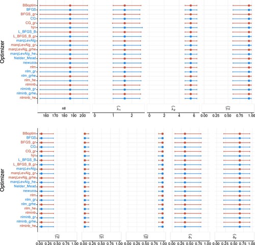
Figure A2. Plots of estimates and NLL when estimating a two-state Poisson HMM in the second study design, with (200 observations), over 1000 realizations. The columns display in order the NLL, Poisson rates, TPM elements, and the stationary distribution. The dots represent the medians, and the lines display the 95% percentile CIs.

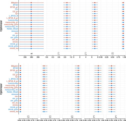
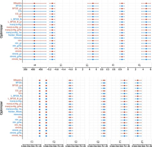
Figure A3. Plots of estimates and NLL when estimating a two-state Poisson HMM in the third study design, with (200 observations), over 1000 realizations. The columns display in order the NLL, Poisson rates, TPM elements, and the stationary distribution. The dots represent the medians, and the lines display the 95% percentile CIs.

Additionally, Tables A4–A6 display the descriptive statistics shown graphically by Figure 13–15.

Table F1. Median duration (in milliseconds and ranked) together with 95% CI and number of iterations required for fitting two-state Poisson HMMs to 200 replications in the first setting.

Optimizer	Median time & CI	Median iteration number & CI	Median time rank
BBoptim	8.49 (5.64, 37.32)	49 (31, 227.2)	18
BFGS	2.22 (1.86, 3.84)		8
BFGS_gr	0.97 (0.81, 1.55)		1
CG	58.73 (23.69, 342.3)		22
CG_gr	30.05 (9.86, 171.94)		21
L-BFGS-B	5.29 (3.69, 8.33)		16
L-BFGS-B_gr	1.65 (1.18, 2.51)		3
Nelder-Mead	4.08 (2.42, 7.38)		15
hjn	10.47 (8.36, 16.63)		19
marqLevAlg	2.99 (2.39, 10.35)	4 (3, 10)	12
marqLevAlg_gr	2.55 (2.03, 9.43)	4 (3, 10)	10
marqLevAlg_grhe	2.41 (2.06, 8.3)	4 (3, 10)	9
marqLevAlg_he	3 (2.37, 10.33)	4 (3, 10)	13
newuoa	5.64 (3.11, 12.19)		17
nlm	2.84 (1.91, 4.27)	21 (13, 31)	11
nlm_gr	1.9 (1.47, 2.55)	21 (13, 31.03)	4
nlm_grhe	3.11 (2.81, 4.07)	4 (3, 7.03)	14
nlm_he	21.87 (14.96, 32.71)	21 (13, 31)	20
nlminb	2.08 (1.7, 2.82)	12 (9, 17)	6
nlminb_gr	1 (0.83, 1.37)	12 (9, 17)	2
nlminb_grhe	2.08 (1.94, 2.61)	4.5 (4, 7)	7
nlminb_he	2.07 (1.73, 2.72)	12 (9, 17)	5

Notes: The CIs are of Wald-type and base on the standard error of the mean derived from 200 replications. A graphical display of these values is available at Figure 13.

Table F2. Median duration (in milliseconds and ranked) together with 95% CI and number of iterations required for fitting two-state Poisson HMMs to 200 replications in the second setting.

Optimizer	Median time & CI	Median iteration number & CI	Median time rank
BBoptim	10.3 (5.56, 24.81)	32 (22, 56.4)	18
BFGS	3.76 (3.08, 8.18)		6
BFGS_gr	1.81 (1.43, 3.89)		1
CG	38.1 (21.46, 94.9)		22
CG_gr	16.81 (8.94, 46.94)		20
L-BFGS-B	6.45 (4.44, 14.42)		16
L-BFGS-B_gr	2.19 (1.47, 4.69)		3
Nelder-Mead	7.17 (3.36, 17.43)		17
hjn	15.43 (10.68, 34.63)		19
marqLevAlg	4.37 (3.37, 9.31)	3 (3, 4)	13
marqLevAlg_gr	3.89 (3.07, 8.36)	3 (3, 4)	7
marqLevAlg_grhe	4.27 (3.6, 8.93)	3 (3, 4)	11
marqLevAlg_he	4.34 (3.4, 9.23)	3 (3, 4)	12
newuoa	6.06 (3.38, 14.03)		15
nlm	3.72 (2.72, 8.55)	16 (11, 19.03)	5
nlm_gr	2.8 (2.22, 6.35)	16 (11, 19)	4
nlm_grhe	5.78 (5.08, 12.73)	3 (2, 4)	14
nlm_he	37.04 (27.75, 83.15)	16 (11, 19.03)	21
nlminb	4.2 (2.94, 9.35)	15 (11, 19)	10
nlminb_gr	2.12 (1.51, 4.82)	15 (11, 19)	2
nlminb_grhe	3.91 (3.34, 8.6)	4 (3, 6)	8
nlminb_he	4.07 (3.05, 9.33)	15 (11, 19)	9

Notes: The CIs are of Wald-type and base on the standard error of the mean derived from 200 replications. A graphical display of these values is available at Figure 14.

Table F3. Median duration (in milliseconds and ranked) together with 95% CI and number of iterations required for fitting two-state Gaussian HMMs to 200 replications in the third setting.

Optimizer	Median time & CI	Median iteration number & CI	Median time rank
BBoptim	59.28 (19.84, 253.76)	84.5 (41, 368.3)	19
BFGS	15.28 (7.21, 19.03)		8
BFGS_gr	5.72 (2.66, 7.22)		1
CG	142.64 (54.48, 290.9)		21
CG_gr	52.84 (21.57, 115.05)		18
L-BFGS-B	34.07 (14.51, 53.75)		16
L-BFGS-B_gr	9.13 (4.07, 14.38)		5
Nelder-Mead	37.41 (13.06, 100.75)		17
hjn	63.68 (30.09, 87.85)		20
marqLevAlg	16.05 (7.49, 38.21)	4 (3, 7.03)	10
marqLevAlg_gr	14.18 (6.75, 35.54)	3 (3, 8)	7
marqLevAlg_grhe	8.64 (4, 29.05)	3 (3, 8)	3
marqLevAlg_he	15.83 (7.42, 35.43)	4 (3, 7.03)	9
newuoa	27.47 (11.32, 43.64)		14
nlm	17.23 (7.92, 22.92)	24 (17.98, 30)	11
nlm_gr	10.86 (5.08, 13.67)	24 (17.98, 30)	6
nlm_grhe	31.3 (14.53, 37.05)	3 (3, 5)	15
nlm_he	228.83 (104.83, 297.81)	24 (17.98, 30)	22
nlminb	18.4 (8.48, 24.52)	21.5 (17, 26)	12
nlminb_gr	7.85 (3.65, 10.17)	22 (17, 26.03)	2
nlminb_grhe	9 (4.21, 11.91)	4 (4, 6.03)	4
nlminb_he	18.4 (8.58, 24.82)	21.5 (17, 26)	13

Notes: The CIs are of Wald-type and base on the standard error of the mean derived from 200 replications. A graphical display of these values is available at Figure 15.

References

- Juang BH, Rabiner LR. Hidden Markov models for speech recognition. Technometrics. 1991 Aug;33(3):251–272. doi: 10.1080/00401706.1991.10484833
- Baum LE, Petrie T. Statistical inference for probabilistic functions of finite state Markov chains. Ann Math Stat. 1966 Dec;37(6):1554–1563. doi: 10.1214/aoms/1177699147
- Rabiner L, Juang B. An introduction to hidden Markov models. IEEE ASSP Mag. 1986 Jan;3(1):4–16. doi: 10.1109/MASSP.1986.1165342
- Rabiner L. A tutorial on hidden Markov models and selected applications in speech recognition. Proc IEEE. 1989 Feb;77(2):257–286. doi: 10.1109/5.18626
- Fredkin DR, Rice JA. Bayesian restoration of single-channel patch clamp recordings. Biometrics. 1992;48(2):427–448. doi: 10.2307/2532301
- Schadt EE, Sinsheimer JS, Lange K. Computational advances in maximum likelihood methods for molecular phylogeny. Genome Res. 1998 Jan;8(3):222–233. doi: 10.1101/gr.8.3.222
- Durbin R. Biological sequence analysis: probabilistic models of proteins and nucleic acids. Cambridge: Cambridge University Press; 1998.
- Eddy SR. Profile hidden Markov models. Bioinformatics. 1998 Jan;14(9):755–763. doi: 10.1093/bioinformatics/14.9.755
- Hamilton JD. A new approach to the economic analysis of nonstationary time series and the business cycle. Econometrica. 1989;57(2):357–384. doi: 10.2307/1912559
- McClintock BT, Langrock R, Gimenez O, et al. Uncovering ecological state dynamics with hidden Markov models. Ecol Lett. 2020;23(12):1878–1903. doi: 10.1111/ele.v23.12
- Lystig TC, Hughes JP. Exact computation of the observed information matrix for hidden Markov models. J Comput Graph Stat. 2002 Sep;11(3):678–689. doi: 10.1198/106186002402
- Ailliot P, Allard D, Monbet V, et al. Stochastic weather generators: an overview of weather type models. J Soc Fr Stat. 2015;156(1):101–113.
- Mor B, Garhwal S, Kumar A. A systematic review of hidden Markov models and their applications. Arch Comput Methods Eng. 2021 May;28(3):1429–1448. doi: 10.1007/s11831-020-09422-4
- Baum LE, Petrie T, Soules G, et al. A maximization technique occurring in the statistical analysis of probabilistic functions of Markov chains. Ann Math Stat. 1970;41(1):164–171. doi: 10.1214/aoms/1177697196
- Dempster AP, Laird NM, Rubin DB. Maximum likelihood from incomplete data via the EM algorithm. J R Stat Soc Ser B (Methodol). 1977;39(1):1–22. doi: 10.1111/j.2517-6161.1977.tb01600.x
- Liporace L. Maximum likelihood estimation for multivariate observations of Markov sources. IEEE Trans Inform Theory. 1982 Sep;28(5):729–734. doi: 10.1109/TIT.1982.1056544
- Wu CFJ. On the convergence properties of the EM algorithm. The Ann Stat. 1983;11(1):95–103. doi: 10.1214/aos/1176346060
- Turner R. Direct maximization of the likelihood of a hidden Markov model. Comput Stat Data Anal. 2008 May;52(9):4147–4160. doi: 10.1016/j.csda.2008.01.029
- MacDonald IL, Zucchini W. Hidden Markov and other models for discrete-valued time series. London: Chapman & Hall; 1997. (Monographs on statistics and applied probability; vol. 70).
- Cappé O, Moulines E, Ryden T. Inference in hidden Markov models. Berlin: Springer Science & Business Media; 2005.
- Lange K, Weeks DE. Efficient computation of lod scores: genotype elimination, genotype redefinition, and hybrid maximum likelihood algorithms. Ann Hum Genet. 1989;53(1):67–83. doi: 10.1111/ahg.1989.53.issue-1
- Zucchini W, MacDonald I, Langrock R. Hidden markov models for time series: an introduction using R. 2nd ed. CRC Press; 2016. (Chapman & Hall/CRC Monographs on Statistics & Applied Probability).
- Altman RM, Petkau AJ. Application of hidden Markov models to multiple sclerosis lesion count data. Stat Med. 2005;24(15):2335–2344. doi: 10.1002/(ISSN)1097-0258
- MacDonald IL. Numerical maximisation of likelihood: a neglected alternative to EM? Int Stat Rev. 2014 Aug;82(2):296–308. doi: 10.1111/insr.v82.2
- Kristensen K, Nielsen A, Berg C, et al. TMB: automatic differentiation and Laplace approximation. J Stat Softw Articles. 2016;70(5):1–21. doi: 10.18637/jss.v070.i05
- Bacri T, Berentsen GD, Bulla J, et al. A gentle tutorial on accelerated parameter and confidence interval estimation for hidden Markov models using template model builder. Biom J. 2022 Oct;64(7):1260–1288. doi: 10.1002/bimj.v64.7
- Gay DM. Usage summary for selected optimization routines. Computing Science Technical Report. 1990;153:1–21.
- Nash JC, Varadhan R. Optimr: a replacement and extension of the optim function; 2019. R package version 2019-12.16; Available from: https://CRAN.R-project.org/package=optimr.
- Bulla J, Berzel A. Computational issues in parameter estimation for stationary hidden Markov models. Comput Stat. 2008 Jan;23(1):1–18. doi: 10.1007/s00180-007-0063-y
- Dennis Jr JE, Moré JJ. Quasi-Newton methods, motivation and theory. SIAM Rev. 1977 Jan;19(1):46–89. doi: 10.1137/1019005
- Schnabel RB, Koonatz JE, Weiss BE. A modular system of algorithms for unconstrained minimization. ACM Trans Math Softw. 1985 Dec;11(4):419–440. doi: 10.1145/6187.6192
- Nelder JA, Mead R. A simplex method for function minimization. Comput J. 1965 Jan;7(4):308–313. doi: 10.1093/comjnl/7.4.308
- Hassan MR, Nath B, Kirley M. A fusion model of HMM, ANN and GA for stock market forecasting. Expert Syst Appl. 2007 Jul;33(1):171–180. doi: 10.1016/j.eswa.2006.04.007
- Stolcke A, Omohundro S. Hidden Markov model induction by Bayesian model merging. Adv Neural Inf Process Syst. 1993;11–11.
- Oudelha M, Ainon RN. HMM parameters estimation using hybrid Baum-Welch genetic algorithm. In: 2010 International Symposium on Information Technology; Vol. 2; Jun.; 2010. p. 542–545. Kuala Lumpur, Malaysia
- Redner RA, Walker HF. Mixture densities, maximum likelihood and the EM algorithm. SIAM Rev. 1984 Apr;26(2):195–239. doi: 10.1137/1026034
- Kato J, Watanabe T, Joga S, et al. An HMM-based segmentation method for traffic monitoring movies. IEEE Trans Pattern Anal Mach Intell. 2002 Sep;24(9):1291–1296. doi: 10.1109/TPAMI.2002.1033221
- Maruotti A, Punzo A. Initialization of hidden Markov and semi-Markov models: A critical evaluation of several strategies. Int Stat Rev. 2021 Dec;89(3):447–480. doi: 10.1111/insr.v89.3
- Michelot T. hmmTMB: Hidden Markov models with flexible covariate effects in R; 2023.
- Feller W. An introduction to probability theory and its applications. New York: Wiley; 1968.
- Pryss R, Reichert M, Langguth B, et al. Mobile crowd sensing services for tinnitus assessment, therapy, and research. In: 2015 IEEE International Conference on Mobile Services; Jun. IEEE; 2015. p. 352–359.
- Pryss R, Reichert M, Herrmann J, et al. Mobile crowd sensing in clinical and psychological trials–a case study. In: 2015 IEEE 28th International Symposium on Computer-Based Medical Systems; Jun. IEEE; 2015. p. 23–24.
- Probst T, Pryss R, Langguth B, et al. Emotion dynamics and tinnitus: Daily life data from the ‘TrackYourTinnitus’ application. Sci Rep. 2016 Aug;6(1):31166. doi: 10.1038/srep31166
- Probst T, Pryss RC, Langguth B, et al. Does tinnitus depend on time-of-day? An ecological momentary assessment study with the ‘TrackYourTinnitus’ application. Front Aging Neurosci. 2017 Aug;9:253. doi: 10.3389/fnagi.2017.00253
- Rydén T, Teräsvirta T, Åsbrink S. Stylized facts of daily return series and the hidden Markov model. J Appl Econom. 1998;13(3):217–244. doi: 10.1002/(ISSN)1099-1255
- Schwert GW. Why does stock market volatility change over time. J Finance. 1989;44(5):1115–1153. doi: 10.1111/j.1540-6261.1989.tb02647.x
- Maheu John M, McCurdy Thomas H. Identifying bull and bear markets in stock returns. J Bus Econ Stat. 2000 Jan;18(1):100–112. doi: 10.1080/07350015.2000.10524851.
- Guidolin M, Timmermann A. Economic implications of bull and bear regimes in UK stock and bond returns. Econom J. 2005 Jan;115(500):111–143. doi: 10.1111/j.1468-0297.2004.00962.x
- R Core Team. R: a language and environment for statistical computing. Vienna, Austria: R Foundation for Statistical Computing; 2021.
- Schwendinger F, Borchers HW. CRAN task view: optimization and mathematical programming. 2022. [Available from: https://cran.r-project.org/view=optimization].
- Broyden CG. The convergence of a class of double-rank minimization algorithms 1. General considerations. IMA J Appl Math. 1970 Mar;6(1):76–90. doi: 10.1093/imamat/6.1.76
- Fletcher R. A new approach to variable metric algorithms. Comput J. 1970 Jan;13(3):317–322. doi: 10.1093/comjnl/13.3.317
- Goldfarb D. A family of variable-metric methods derived by variational means. Math Comput. 1970;24(109):23–26. doi: 10.1090/mcom/1970-24-109
- Shanno DF. Conditioning of quasi-Newton methods for function minimization. Math Comput. 1970;24(111):647–656. doi: 10.1090/mcom/1970-24-111
- Byrd RH, Lu P, Nocedal J, et al. A limited memory algorithm for bound constrained optimization. SIAM J Sci Comput. 1995 Sep;16(5):1190–1208. doi: 10.1137/0916069
- Fletcher R. Practical methods of optimization. Hoboken, New Jersey, U.S.A: John Wiley & Sons; 2013.
- Dennis JE, Schnabel RB. Numerical methods for unconstrained optimization and nonlinear equations. Society for Industrial and Applied Mathematics; 1996. (Classics in Applied Mathematics).
- Hooke R, Jeeves TA. ‘Direct search’ solution of numerical and statistical problems. J ACM. 1961 Apr;8(2):212–229. doi: 10.1145/321062.321069
- Philipps V, Proust-Lima C, Prague M, et al. Marqlevalg: a parallelized general-purpose optimization based on marquardt-levenberg algorithm; 2023. R package version 2.0.8; Available from: https://CRAN.R-project.org/package=marqLevAlg.
- Levenberg K. A method for the solution of certain non-linear problems in least squares. Quart Appl Math. 1944;2(2):164–168. doi: 10.1090/qam/1944-02-02
- Marquardt DW. An algorithm for least-squares estimation of nonlinear parameters. J Soc Indust Appl Math. 1963 Jun;11(2):431–441. doi: 10.1137/0111030
- Varadhan R, Gilbert P. Bb: solving and optimizing large-scale nonlinear systems; 2019. R package version 2019.10-1; Available from: http://www.jhsph.edu/agingandhealth/People/Faculty_personal_pages/Varadhan.html.
- Varadhan R, Gilbert P. BB: an R package for solving a large system of nonlinear equations and for optimizing a high-dimensional nonlinear objective function. J Stat Softw. 2010;32:1–26. doi: 10.18637/jss.v032.i04
- Bates D, Mullen KM, Nash JC, et al. minqa: derivative-free optimization algorithms by quadratic approximation; 2022. R package version 1.2.5; Available from: http://optimizer.r-forge.r-project.org.
- Powell MJD. The NEWUOA software for unconstrained optimization without derivatives. In: Di Pillo G, Roma M, editors. Large-scale nonlinear optimization. Boston (MA): Springer US; 2006. p. 255–297. (Nonconvex Optimization and Its Applications).
- Mersmann O. microbenchmark: accurate timing functions; 2023. R package version 1.4.10; Available from: https://github.com/joshuaulrich/microbenchmark/.
- Böhning D. Computer-assisted analysis of mixtures and applications: meta-analysis, disease mapping and others. Vol. 81. Boca Raton, Florida: CRC press; 1999.
- Bhatia R, Davis C. A better bound on the variance. Am Math Mon. 2000 Apr;107(4):353–357. doi: 10.1080/00029890.2000.12005203
- Nagy J. Über algebraische Gleichungen mit lauter reellen Wurzeln. Jahresbericht Der Deutschen Mathematiker-Vereinigung. 1918;27:37–43.
- Biernacki C, Celeux G, Govaert G. Assessing a mixture model for clustering with the integrated completed likelihood. IEEE Trans Pattern Anal Mach Intell. 2000 Jul;22(7):719–725. doi: 10.1109/34.865189
- Visser I, Raijmakers MEJ, Molenaar PCM. Confidence intervals for hidden Markov model parameters. British J Math Stat Psychol. 2000;53(2):317–327. doi: 10.1348/000711000159240
- Pawitan Y. In all likelihood: statistical modelling and inference using likelihood. Oxford: Oxford University Press; 2001.
- Zheng N, Cadigan N. Frequentist delta-variance approximations with mixed-effects models and TMB. Comput Stat Data Anal. 2021 Aug;160:107227. doi: 10.1016/j.csda.2021.107227
- Efron B, Tibshirani RJ. An introduction to the bootstrap. New York (NY); London: Chapman & Hall; 1993.
- Härdle W, Horowitz J, Kreiss JP. Bootstrap methods for time series. Int Stat Revi. 2003;71(2):435–459. doi: 10.1111/insr.2003.71.issue-2