3D vegetation mapping using small‐footprint full‐waveform airborne laser scanners

Abstract

Small‐footprint full‐waveform airborne laser scanning (ALS) is a remote sensing technique capable of mapping vegetation in three dimensions with a spatial sampling of about 0.5–2 m in all directions. This is achieved by scanning the laser beam across the Earth's surface and by emitting nanosecond‐long infrared pulses with a high frequency of typically 50–150 kHz. The echo signals are digitized during data acquisition for subsequent off‐line waveform analysis. In addition to delivering the three‐dimensional (3D) coordinates of scattering objects such as leaves or branches, full‐waveform laser scanners can be calibrated for measuring the scattering properties of vegetation and terrain surfaces in a quantitative way. As a result, a number of physical observables are obtained, such as the width of the echo pulse and the backscatter cross‐section, which is a measure of the electromagnetic energy intercepted and re‐radiated by objects. The main aim of this study was to build up an understanding of the scattering characteristics of vegetation and the underlying terrain. It was found that vegetation typically causes a broadening of the backscattered pulse, while the backscatter cross‐section is usually smaller for canopy echoes than for terrain echoes. These scattering properties allowed classification of the 3D point cloud into vegetation and non‐vegetation echoes with an overall accuracy of 89.9% for a dense natural forest and 93.7% for a baroque garden area. In addition, by removing the vegetation echoes before the filtering process, the quality of the digital terrain model could be improved.

1. Introduction

Two‐dimensional (2D) images of the Earth's surface collected by sensors onboard airborne or spaceborne platforms are a valuable source of data for mapping vegetation. The most commonly used remote sensing technique for mapping vegetation is multispectral imaging, using either photographic or digital means in the visible and infrared portions of the electromagnetic spectrum. At microwave frequencies, synthetic aperture radar (SAR) techniques are used to create high‐resolution images of the backscattered radiation. These images are 2D representations of the recorded radiation, where each image pixel represents an area on the ground. One problem of 2D imaging over vegetated terrain is that, even at the high spatial resolutions offered by airborne spectral imagers, there are typically different vegetation elements (leaves, branches, etc.) at different heights above the ground surface within the resolution cell of the sensor. 2D imaging techniques do not allow differentiation between these vegetation elements and the recorded signals depend strongly on the geometric arrangement of the vegetation elements and the illumination conditions (Liang 2004). This makes classification of 2D images challenging because the received signal can vary substantially depending on the exact geometric composition of the vegetation elements even within one particular vegetation class. In addition, the retrieval of geophysical parameters such as leaf area index (LAI) is a challenging task as models are required to extract contributions from different vegetation layers and the ground surface.

Many of these fundamental limitations of 2D imaging techniques may be overcome by 3D measurement techniques that allow separation of objects found at different heights above the Earth's surface. Particularly for vegetation mapping purposes, the advantages of 3D imaging techniques are significant. In geophysical parameter retrieval, separate models can be used for the ground surface and different vegetation layers, thus reducing the complexity of the retrieval process. In classification, the height information and spatial relationships of objects captured by 3D techniques can be used in a synergistic way with the radiometric (spectral) information to improve the accuracy and robustness of the classification procedure. The powerful capabilities of such an approach have been demonstrated over an urban area by Zebedin et al. (2006), who used a multiple‐image matching technique to derive height information from multispectral airborne imagery.

Multi‐image matching refers to a technique to extract 3D information from two or more 2D images taken at different positions and is an extension of classical stereoscopic methods. Over vegetated areas the challenge lies in finding corresponding points in at least two images that are the projections of the same vegetation point. Felicísimo and Cuartero (2006) proposed using the spectral information of remote sensing images to improve the matching process. Zhang and Grün (2006) demonstrated that high‐quality digital surface models can be obtained for forested areas by using a coarse‐to‐fine hierarchical solution and multiple matching primitives. Because of shadow and occlusion, the matching of vegetation points becomes increasingly difficult for lower canopy layers and the underlying ground surface. Therefore, in practice, multi‐image matching techniques are suitable for describing the top canopy layers but provide only limited information about the lower canopy layers and the underlying terrain.

Active remote sensing techniques are more capable of resolving the vertical structure of vegetation. Particularly suited are radar (radio detection and ranging) systems that can penetrate the vegetation because of their long wavelength (centimetre to decimetre waves). For example, Hyyppä et al. (1997) used a helicopter‐borne ranging scatterometer operating at two wavelengths (3.1 cm and 5.4 cm) to measure the backscattering characteristics of forest stands as a function of height with a vertical resolution of about 0.65 m along the flight line. Spaceborne SAR systems can be used for 3D mapping of large areas by processing more than two SAR images to synthesise an aperture in elevation (Reigber and Moreira 2000, She et al. 2002, Fornaro et al. 2005). However, further research is still needed to assess the practical use of this technique for vegetation mapping.

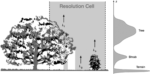
Another active remote sensing technique capable of resolving the vertical structure of vegetation is light detection and ranging (lidar), here generally referred to as laser scanning. Laser scanners emit short pulses of electromagnetic radiation in the infrared and sometimes the visible region of the spectrum towards the Earth's surface and record the backscattered echoes (figure 1). A disadvantage of lidar compared to radar techniques is that laser pulses can penetrate the vegetation canopy only through gaps, which means that below the dense crown layers very little information about the ground surface and deeper canopy layers is obtained. However, laser scanners can more easily achieve a fine resolution in both the horizontal and vertical directions.

Figure 1 By illuminating vegetation with short pulses of laser light, the vertical profile of the vegetation can be resolved. The diagram on the right shows the echo received by a full‐waveform airborne laser scanner for the situation depicted on the left. Note that 2D imaging systems are not able to differentiate between the radiation originating from different objects within the horizontal resolution cell. In this example, 2D imagers record the sum of radiation stemming from the tree (L _t), the shrub (L _s), and the ground (L _g).

Lidar instruments have been mounted on spaceborne and airborne platforms. The technical feasibility of full‐waveform digitizing lidar instruments was demonstrated by large‐footprint airborne systems developed by the National Aeronautics and Space Administration (NASA) in the 1990s (Blair et al. 1999). Even though the laser footprint was of the order of tens of metres depending on the flying altitude, it soon became clear that this technique can reveal important information about the canopy structure (Harding et al. 2001) because of the fine vertical resolution, which is of the order of about 0.5–2 m. More recently, NASA has also developed a small‐footprint (∼20 cm) waveform digitizing airborne lidar instrument called Experimental Airborne Advanced Research Lidar (EAARL) for mapping near‐shore bathymetry, topography and vegetation structure simultaneously (Nayegandhi et al. 2006). EAARL emits very short laser pulses (1.2 ns) and is hence able to resolve the vertical vegetation structure with a resolution of 18 cm. Spaceborne full‐waveform data over land have been delivered by the Geoscience Laser Altimeter System (GLAS) onboard the Ice Cloud and land Elevation Satellite (ICESat) (Zwally et al. 2002). Harding and Carabajal (2005) discuss how, in addition to vegetation structure, subfootprint topographic height variations affect the GLAS waveform over land due to the large footprint size of GLAS (66 m).

Commercial small‐footprint airborne laser scanner systems with full‐waveform digitizing capabilities have recently become available. The potential of these sensors was demonstrated by Hug et al. (2004) based on waveform data acquired with the LMS‐Q560 manufactured by Riegl (www.riegl.com), by Persson et al. (2005) using the Mark II system of Blom Sweden (formerly TopEye, www.topeye.com), and by Gutierrez et al. (2005) for the ALTM waveform digitizer of Optech (www.optech.ca). The system waveform of these sensors is typically very similar to an ideal Gaussian function with a pulse width at half maximum of about 4–8 ns. Wagner et al. (2006) presented the theoretical basis for decomposing the recorded small‐footprint waveform into a series of Gaussian pulses and for calculating the backscatter cross‐section for each individual echo. In the present study these methods are applied over a park area to build up an understanding of the characteristics of full‐waveform data over vegetated terrain. One particular issue was how well full‐waveform laser scanners can distinguish between ground hits and echoes from low and high vegetation. Furthermore, a new method for improving the quality of digital terrain models (DTMs) in vegetated areas was applied as a means for more accurate modelling of canopy height.

2. Sensor

Airborne laser scanning (ALS) is an active remote sensing technique originally developed for topographic data acquisition that performs the sampling of the landscape stripwise in a dynamic way. Short laser pulses (typically 4–10 ns) are emitted with a high frequency (typically 50–150 kHz) and are deflected continuously across the flight direction towards the Earth's surface. After the interaction of the laser pulse with the object surface, some of the energy may be scattered back to the sensor. The echo is detected by a synchronized receiver situated on the laser scanning unit. As a result, the round‐trip time between the sensor and the Earth's surface is determined and the distance (range) to the object can be calculated with the knowledge of the velocity of the light package. Additional to the object distance, the angle of deflection is recorded per pulse. The time‐dependent position and orientation of the sensor system is observed using a synchronized Position and Orientation System (POS) that normally consists of a Global Positioning System (GPS) and an Inertial Measurement Unit (IMU). Based on all the synchronized observations, the 3D coordinates of all detected objects can be determined in post‐processing within one coordinate frame with a high accuracy (Ackermann 1999, Wehr and Lohr 1999).

Most currently operating ALS systems provide the 3D coordinates of the laser point cloud and intensity information. If several objects are illuminated by one laser pulse, a complex interaction of the laser beam with the illuminated object surface can be observed (figure 1). Depending on the sensor, the range of two echoes (first and last) or multiple echoes (up to five) can be recorded. Scattering objects produce distinct echoes if they are separated by a distance

or larger, where v _g is the group velocity of the laser pulse and τ is the pulse duration. The parameter r _R is called the range resolution and defines the shortest separation of objects that can be measured. Because in ALS the scan angle is limited to close‐nadir views (typically ±20°), this value also defines the vertical resolution of the measurement system. Some ALS systems have a dead‐zone of 3 m or more after a detected echo, and their vertical resolution is in practice smaller than that given by equation (1).

The intensity information provided by ALS systems describes the amount of backscattered pulse energy. As noted previously by Lim et al. (2003), up to now little emphasis has been placed on how the intensity information can be used as source of information for vegetation applications. Possibly, this is partly because the recorded intensity values are often fairly noisy and not well defined. Most of the subsequent modelling procedures for deriving terrain or vegetation models therefore focus purely on geometric and topologic relationships of the irregularly distributed 3D point cloud.

The novel full‐waveform digitizing small‐footprint ALS systems have the advantage that the measurement process is depicted in its entire complexity (Wagner et al. 2006). This opens the possibility of deriving physical observables in addition to the range. In this study waveform data acquired with the Riegl LMS‐Q560 were analysed. The most important instrument specifications are summarized in table 1. The sensor has a Gaussian‐shaped system waveform with a width at half maximum of 4 ns. Thus the vertical resolution is about 0.6 m according to equation (1). The received echo waveform was sampled with a time interval of 1 ns. This corresponds to a sampling distance of about 15 cm in the vertical direction.

Table 1. Main technical specifications of the RIEGL LMS‐Q560.

Operating altitude	<1500 m
Wavelength	1.5 µm
Pulse width at half maximum	4 ns
Pulse energy	8 µJ
Pulse firing rate	<100 kHz
Laser beamwidth	0.5 mrad
Scan angle range	±22.5°
Footprint size	0.5 m×1 km
Digitizer	1 ns

The waveform measured by full‐waveform lidar instruments is often modelled as a series of Gaussian pulses (Hofton et al. 2000, Persson et al. 2005). As the system waveform of LMS‐Q560 can be approximated by a Gaussian‐shaped pulse, this approach is also applicable to LMS‐Q560 data. The received waveform P _r(t) can be written as:

where t_i is the round‐trip time, s _p,i the standard deviation of the echo pulse, the amplitude of target i, and N the number of targets within the travel path of the laser pulse. Figure 2 presents an example of a complex waveform caused by several backscattering objects within the travel path of the laser pulse. The figure shows the recorded waveform, the individual Gaussian functions per detected echo, and the overall fitted model. Four distinct echoes at different ranges were determined in this case, and the distance between the first three echoes is fairly short (especially between echos two and three). The fitted model parameters (i.e. amplitude, echo width, and distance (range)) are given in table 2.

Figure 2 Gaussian decomposition of the LMS‐Q560 waveform showing the recorded waveform (points), the Gaussian functions for all four detected echoes (broken lines), and the overall fitted model (solid line). The model parameters of the individual echo pulses are given in table 2.

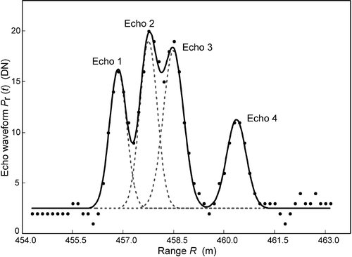
Table 2. Results of Gaussian decomposition of the echo waveform shown in figure 2.

Echo ID	Range (m)	Amplitude (DN)	Echo width (ns)	Backscatter cross‐section (m^2)
1	456.91	13.73	1.70	0.01456
2	457.82	16.52	1.74	0.01807
3	458.55	15.60	2.02	0.01994
4	460.42	8.78	1.94	0.01096

3. Theory

The echo waveform received by full‐waveform ALS systems is the result of a convolution of the system waveform and the backscattering cross‐section of the illuminated object surface (Jutzi and Stilla 2006). The backscattering cross‐section (in units of square metres) is a measure of the electromagnetic energy intercepted and re‐radiated by objects backwards towards the sensor. It is a fundamental quantity in radar and lidar remote sensing and can be determined analytically by solving Maxwell's equation (Toomay and Hannen 2004) and experimentally by calibrating laser scanner measurements (Wagner et al. 2006). It thus constitutes a bridge between theory and measurements and should become a standard product in laser scanning. As shown in Wagner et al. (2006), the backscatter cross‐section can be calculated for each echo based on the model parameters obtained by the Gaussian waveform decomposition:

where σ _i is the backscatter cross‐section of target i, R_i the range between sensor and target i, and C _Cal is the calibration constant. An asphalt road was used for determining the calibration constant. It was assumed that the asphalt road behaves like an ideal Lambertian scatterer with a reflectivity of 0.2. For a more accurate calibration several brightness targets with nominal reflectance values could be deployed before the flight, as demonstrated by Kaasalainen et al. (2005) and Ahokas et al. (2006).

As its name suggests, the cross‐section is the effective area of collision of the laser beam and the target, taking into account the directionality and strength of reflection. It can be written as (Jelalian 1992):

where Ω _i is the scattering solid angle of the target in steradians, ρ _i is the reflectivity of the target, and A_i is the effective area of collision of target i located at (x_i , y_i , z_i ). Because in ALS the wavelength is always much smaller than the size of the targets, A_i is simply the projected area of the scatterer. For an extended target that is larger than the footprint size of the laser beam, the collision area is equal to the footprint area A _f. Such a target obviously produces only a single echo. For targets that have a smooth surface compared to the laser wavelength, the laser pulse may be reflected specularly away from the sensor, in which case no echo signal is recorded (Schanda 1986). Examples are reflections by artificial materials such as glass or polished metals and calm water surfaces.

Let us now consider multi‐echo waveforms over vegetated terrain. Because vegetation, soil and other natural objects have a rough surface at infrared wavelengths that results in diffuse scattering in all directions, it is reasonable to assume that each target hit by the laser pulse scatters some energy backwards towards the sensor. Then the total backscatter cross‐section σ_t per laser shot is given by:

where N is the number of targets. This parameter describes how much energy is scattered backwards towards the sensor from the laser footprint area centred at (x, y). It is closely related to the backscattering coefficient commonly used in SAR imaging. Note that σ_t is a 2D parameter: that is, the height information is lost. As for single‐echo waveforms, the total area of collision of multi‐echo waveforms must be equal to the footprint area A _f if there are no specular reflecting targets. Therefore

where A_i is the area of collision of the ith target. This simple relationship helps in understanding the signal strength of multi‐echo waveforms. Let us consider a waveform with two distinct echoes with cross‐sections σ₁ and σ₂. It is known that A ₁+A ₂ = A _f. Therefore, the cross‐section of the second target depends on the cross‐section of the first target:

This equation shows that with increasing collision area of the first target, A ₁, the cross‐section of the second target is expected to decrease, and vice versa. It also suggests that σ₂ can be predicted from σ₁ using a prediction function ξ(σ₁):

Comparison of equations (7) and (8) shows that the prediction function should be of following form:

where c ₁ and c ₂ are two constants that depend on the scattering characteristics of the two targets. If it is assumed that the two echoes are produced by one target type characterized by similar scattering characteristics, i.e. Ω₁≈Ω₂ = Ω and ρ₁≈ρ₂ = ρ, then the predictor function becomes:

where σ_t is the characteristic total cross‐section of this target type. Because Ω₁ and Ω₂ and respectively ρ₁ and ρ₂ will never be exactly the same, equation (10) accounts for the situation that σ₁ is larger than the characteristic total cross‐section σ_t. Extending these considerations to three or more targets shows that, with an increasing number of detected targets, we can expect all σ _i values to decrease compared to single echoes from the corresponding targets. If all echoes are generated by one target type, the strength of single echoes is simply a function of the area of collision and the total cross‐section:

Of course, the condition that the Ω _i and respectively the ρ _i values are identical for all echoes in multi‐modal waveforms cannot be met exactly, even for forest canopies with a homogeneous vertical distribution of scatterers. Therefore, equations (10) and (11) should not be regarded as deterministic relationships. Rather, they serve to illustrate some general scattering principles as a means to facilitate the interpretation of full‐waveform ALS data.

4. Methods

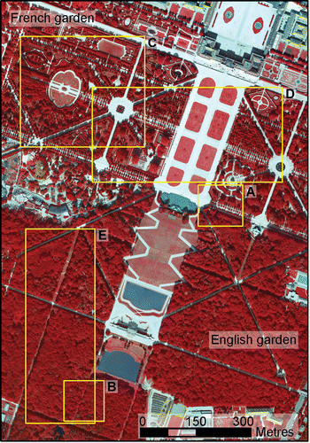
To analyse the information content of full‐waveform ALS data over vegetated areas, we processed LMS‐Q560 data over the park area of the Schönbrunn Palace in Vienna, Austria, located atound 16°18′44″ E and 48°10′59″ N at 160 m height above sea level. The park is divided into two parts (figure 3). The northern part, the so‐called French garden, is a baroque garden. The branches of trees and shrubs along the roads are cut annually. The main tree species in this part are linden (Tilia sp.), maple (Acer sp.) and sycamore (Platanus sp.). There is also sparse occurrence of English yew (Taxus baccata), beech (Fagus sylvatica) and chestnut (Aesculus hippocastanum). The age of the trees ranges between 20 and 200 years. In the southern part of the park, the so‐called English garden, the vegetation is more or less left in its natural condition. Dead or damaged trees are not removed from this forest. The main tree species are oak (Quercus sp.), ash (Fraxinus excelsior) and maple (Acer sp.). Some linden (Tilia sp.), hornbeam (Carpinus betulus) and occasionally cherry (Prunus sp.) and poplar (populus sp.) occur. All these species form the natural vegetation due to the environmental conditions. Most of the trees are old, between 150 and 220 years old. The height of the upper tree layer is around 25 m.

Figure 3 Colour‐infrared image of Schönbrunn Park. In the northern part the so‐called French garden can be seen. The forest in the southern part of the park area is referred to as the English garden. The yellow boxes indicate test and validation areas: A, area shown in figure 4 (110 m×110 m); B, area shown in figure 5 (110×110 m); C, area shown in figure 10 (340 m×300 m); D, validation area in the French garden (515 m×255 m); and E, validation area in the English garden (190 m×525 m).

The LMS‐Q560 data were acquired during leaf‐on conditions on 30 August 2004 by Milan‐Flug (Wagner et al. 2006). The flying height was 500 m above ground and the scan rate was set to 66 kHz. This resulted in a laser footprint size on the ground of about 25 cm and an approximate mean point density of four measurements per square metre, which corresponds to a mean sampling distance of about 0.5 m. To support the interpretation of the LMS‐Q560 data, the same area was imaged with the Vexcel UltraCam‐D multispectral digital aerial camera by Vermessung Meixner in cooperation with Bildflug Fischer one week later, on 9 September 2004. Flight altitude was about 1150 m above ground and pixel size on the ground was about 10.2 cm in the panchromatic channel and about 30 cm in the four spectral channels (RGB and near‐infrared). The processing of the LMS‐Q560 data was accomplished in three steps: (1) exact georeferencing according to the methods described in Kager (2006); (2) Gaussian decomposition and calibration as described in Wagner et al. (2006); and (3) filtering of the data for generating a DTM following the novel, full‐waveform‐based method proposed by Doneus and Briese (2006).

The improvement in DTMs in vegetated areas is an indirect but important means for improving the vegetation characterization with ALS data (Hollaus et al. 2006). In the past few years many different algorithms have been developed that filter the ALS point cloud to eliminate off‐terrain points (Sithole and Vosselman 2004). All these approaches have in common the fact that they rely only upon geometric criteria (typically the height relationship of neighboured points) for the elimination of off‐terrain points. Besides problems with large off‐terrain objects and surface discontinuities, these algorithms often have problems with filtering low vegetation, bushes and tree‐trunks (Pfeifer et al. 2004). Therefore, the DTM surface may run through the lowest canopy levels in these areas. The fundamental reason for this problem is that conventional ALS systems cannot distinguish objects from the ground surface if these objects are shorter than the range resolution given by equation (1). Also, in full‐waveform ALS such objects do not produce distinguishable echoes. However, they lead to a broadening of the received waveform and can hence be eliminated. Following this reasoning, Doneus and Briese (2006) proposed a two‐step approach for DTM generation. In the first step, all last echo points with a significantly greater echo width than the echo width of the system waveform are eliminated using a simple threshold value. In the second step, a standard filtering procedure as described by Kraus and Pfeifer (1998) and Briese et al. (2002) is used for classifying the remaining points into terrain and off‐terrain points.

For exploratory analysis of the full‐waveform data, 2D and 3D visualizations of the different observables were created, including displays of the number of echoes per laser shot, the total cross‐section σ_t, and the four observables available for each echo (i.e. range R, amplitude , echo width s _p and cross‐section σ). For a more quantitative assessment of the discriminatory power of the different observables, histograms were created for different target types (forest canopy, forest floor, grass, gravel) by manual selection of training areas and by using height thresholds with respect to the terrain surface. Scatterplots were also produced to study the relationship between cross‐sectional values of single‐ and multi‐echo waveforms. Guided by the insights gained from this exploratory analysis, a simple decision tree was defined to automatically distinguish vegetation from terrain points. The results of the classification process were evaluated separately for areas within the French and English gardens. Height thresholds were again used as criteria for ascertaining and rejecting the correctness of the classification of individual echoes.

5. Results and discussion

5.1 General behaviour of full‐waveform parameters

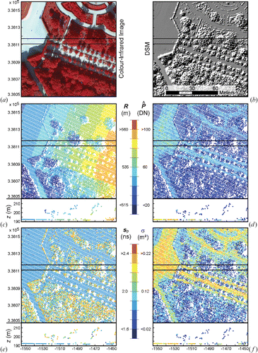
A visual comparison of the full‐waveform parameters with the colour‐infrared image and a shaded digital surface model (DSM) is shown in figure 4. The scene shows a small area within the French garden. The flight line of the laser scanner was in the north–south direction westward of this area. As a result, the range R increases from the left to the right of the image and there are shadow regions (areas without ALS points) on the right side of some of the trees. The amplitude image exhibits comparably low contrast, with slightly higher values observed over the gravel road. By contrast, the echo width allows us to distinguish smooth surfaces from plants, bushes and trees very clearly. Even some of the short hedges (<0.5 m) can be recognized in the pulse width image. The cross‐section image shows some contrast between the gravel road, grass and the higher vegetation points, albeit not as pronounced as for the pulse width. Figure 4 also offers side views of all observables for the east–west profile indicated in the nadir‐view images. We can see that many of the free‐standing trees have a dense canopy, with most laser shots producing only one detectable echo. Nevertheless, some laser pulses penetrate to the ground. They produce in general only a weak echo because a fraction of the pulse energy has already been scattered and absorbed by the overlying canopy.

Figure 4 3D observables obtained by Gaussian decomposition of full‐waveform airborne laser scanner (ALS) data: (a) colour‐infrared image; (b) shaded digital surface model (DSM); (c) nadir view (above) and side view of selected profile (below) of range R in m; (d) nadir view (above) and side view of selected profile (below) of echo amplitude in digital numbers (DN); (e) nadir view (above) and side view of selected profile (below) for echo width s _p in ns; (f) nadir view (above) and side view of selected profile (below) for cross‐section σ in m².

The scattering properties of the forest in the English garden are illustrated in figure 5. A narrow grass‐covered aisle crosses the scene from north‐east to south‐west. Even though the forest is very dense, many ground hits can be observed. Figure 5(b) also shows that there are more multi‐echo than single‐echo returns over this forest. As expected, the cross‐section of individual echoes depends strongly on the number of echoes. Therefore, the cross‐section of single‐echo returns is generally stronger than the cross‐section of multiple echoes. As the last echo σ_last over the forest is generally weak, the forest aisle can clearly be recognized in the σ_last image shown in figure 5(c) .

Figure 5 Illustration of relationship between number of echoes and cross‐section over a forest area: (a) colour‐infrared image; (b) number of single‐echo (black dots) and multi‐echo (green dots) waveforms; (c) nadir view (above) and side view of selected profile (below) of cross‐section of the last echo σ_last; (d) nadir view (above) and side view of selected profile (below) for the total backscatter cross‐section σ_t projected onto the last echo point.

5.2 Cross‐section of vegetation and terrain echoes

The total cross‐section σ_t image shown in figure 5(d) exhibits some interesting patterns. To understand whether, and how, the number of pulses and the forest floor influence σ _t , the histogram plots shown in figure 6 were created. The left diagram (figure 6(a) ) shows σ_t‐histograms of waveforms with echoes originating solely from within the forest canopy. We can see that the σ_t‐histograms of the waveforms with either one‐, two‐ or three‐canopy echoes are almost identical. The mean σ_t is 0.069 m² and the standard deviation is 0.019 m². The impact of the forest floor on σ_t is illustrated by the histograms shown in figure 6(b) . In this forest site the echo from the ground is generally stronger (mean value of 0.12 m²) than the echo from the canopy. Therefore, the σ_t‐histograms of the mixed waveforms with both canopy and terrain echoes take on an intermediate position. To summarize, while scattering contributions from the forest floor are responsible for some of the spatial patterns in the σ_t image shown in figure 5( d), the number of canopy echoes has no such impact. In addition to terrain contributions, the projection of σ_t values into the position of the last echo as displayed in the side view of figure 5( d) shows that σ_t also varies within the forest canopy layer, probably influenced by tree species and tree structure. As the results obtained by Reitberger et al. (2006) suggest, this parameter may be useful for tree species classification.

Figure 6 Histograms of the total backscatter cross‐section σ_t for waveforms observed over a forest: (a) σ_t of echoes stemming from within the forest canopy; (b) σ_t of forest waveforms where the last echo is from the ground surface.

Let us now regard the strength of individual echoes from the forest canopies. As expected, the sequence of σ _i ‐histograms of waveforms with one, two or three canopy echoes shows that the individual echoes become weaker with an increasing number of echoes (figure 7). Unlike the more Gaussian‐shaped histograms of the total cross‐section, the σ _i ‐histograms of waveforms with two‐ and three‐canopy echoes are strongly skewed. Also as expected from our discussion in section 3, the strength of the second (and higher‐order) canopy echoes depends on the strength of the first (previous) echos. Figure 8 shows the observed predictor function for waveforms with two canopy echoes. The scattering of points is relatively large, probably because no distinction between different tree species was made in the selection of the data set from which this plot was generated. Nevertheless, it follows a hyperbolic function as predicted by equation (9). As the total cross‐section of the forest canopies is independent of the number of echoes (figure 6( a)), it further appears to be a reasonable assumption that the scattering properties of different canopy layers are comparable, which leads us to equation (10). By substituting the observed mean value of the total cross‐section of forest canopies into equation (10) and plotting the resulting curve in figure 8, a reasonable fit is indeed found.

Figure 7 Histograms of the backscatter cross‐section σ _i for waveforms observed over (a,b,c) forest and (d) open terrain (grass, gravel). The histograms for forest only show waveforms with echoes from within the forest canopy (i.e. returns from the forest floor are not included). The three forest histograms show the cases of (a) one‐, (b) two‐ and (c) three‐echo waveforms, respectively.

Figure 8 Prediction function of second forest canopy echo(σ₂) based on the first echo (σ₁).

Finally, we note that the cross‐section of the vegetation echoes is in general lower than for the terrain echoes. It is already known from figure 6( b) that the cross‐section of the forest floor is generally higher than the total cross‐section of the canopy echoes. Furthermore, figure 7( d) shows that gravel produces a much stronger backscatter signal with a mean cross‐section value of 0.18 m². Grass produces echoes of somewhat higher, but still comparable, strength (0.098 m²) than forest canopies, which is probably the result of similar reflectivity characteristics. These characteristics of the cross‐section may make it possible to automatically distinguish terrain from vegetation echoes without considering geometric and topologic relationships of the 3D point cloud.

5.3 Width of echoes from vegetation and terrain

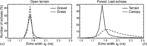
Using waveform data of a forest site in Sweden recorded with the TopEye Mark II system, Persson et al. (2005) found that the width of vegetation echoes tends to be larger than that of terrain echoes. This is confirmed by the histograms in figure 9. We can see that the echo width is fairly narrow (similar to the pulse width of the emitted beam) in open terrain, including gravel and grass, whereas the increase in the echo width of points in the canopy is clearly visible. The resulting distribution of the echo width parameter in the vegetation canopy is asymmetric and shifted towards higher echo width values. In contrast to these canopy points, the distribution of the echo width of the terrain points in the forest area is similar to that over open terrain. This suggests that, despite the partial overlap of the histograms of the canopy and terrain echoes, the echo width is a useful indicator for discriminating canopy and terrain echoes. However, the estimation of the echo width is less accurate for weak echoes compared to strong ones (Wagner et al. 2006). Therefore, the echo width of data below the vegetation canopies must be treated with care. Additionally, we have to consider that in areas of steep terrain, the echo can be wide due to a grazing incidence of the laser pulse.

Figure 9 Histograms of the echo width over open terrain and forest: (a) grass and gravel echoes; (b) terrain and canopy echoes in forest.

5.4 Classification of vegetation echoes

Based on these findings a simple decision tree approach was established to evaluate whether the classification of vegetation echoes can be performed automatically based solely on the full‐waveform observables. In the first step of this process, all last echo points with an echo width larger than 1.9 ns and a total cross‐section of less than 0.08 m² are classified as vegetation echoes. Then all other points (first and intermediate echoes) are also allocated to the class vegetation. The result of this simple approach is presented in figure 10. It can be seen that besides points on trees, points on bushes, hedges and even on very low flower arrangements could also be identified. Error matrixes as discussed by Congalton and Green (1999) were computed for validation areas (figure 3) in the French garden (table 3) and the natural forest in the English garden (table 4). Besides the classification accuracies and errors of commission and omission, the κ‐value was also calculated as another measure of the classification accuracy that takes chance agreement into account. As seen in table 3, the overall classification accuracy was 93.7% with a κ‐value of 0.86 for the French garden. Overall, the natural forest accuracy was also fairly high (89.8%) but the κ‐value was significantly lower (0.57).

Figure 10 Classification of 3D laser scanner point cloud and improved digital terrain model(DTM) filtering using full‐waveform data: (a) shaded digital surface model; (b) classified vegetation echoes (black dots) overlaid over a shaded digital surface model; (c) DTM without exploiting full‐waveform information; (d) improved DTM by using of full‐waveform information.

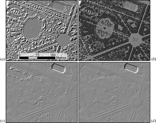
Table 3. Error matrix for the validation area in the French garden.

Classified data	Reference
	Terrain	Vegetation	Total	User's accuracy (%)
Terrain	88 664	3112	91 776	96.6
Vegetation	5890	44 870	50 760	88.4
Total	94 554	47 982	142 537
Producer's accuracy (%)	93.8	93.5
Overall accuracy: 93.7%		Kappa: 0.86

Table 4. Error matrix for the validation area in the English garden.

Classified data	Reference
	Terrain	Vegetation	Total	User's accuracy (%)
Terrain	15 090	10 652	25 742	58.6
Vegetation	7354	143 037	150 391	95.1
Total	22 444	153 689	176 134
Producer's accuracy (%)	67.2	93.1
Overall accuracy: 89.8%		Kappa: 0.57

5.5 DTM generation using full‐waveform information

The full‐waveform‐based DTM filtering method proposed by Doneus and Briese (2006) was originally developed for a rural, predominantly forested area. It also worked satisfactorily over the Schönbrunn park area as illustrated by figure 10. This figure compares the DTMs generated by hierarchic robust interpolation with and without consideration of the full‐waveform information. In figure 10( c), shading of the DTM after applying the standard filtering process based on geometric considerations is presented, and in figure 10( d) the result of the advanced filtering procedure is illustrated. It is clearly visible that the DTM after standard processing contains small bulges stemming from diverse objects such as roses or shrubs. The model generated with the additional pre‐elimination of the points with a large echo width is much smoother. It represents the terrain surface in a more realistic way and can serve as a better basis for the subsequent determination of the height of low vegetation species.

6. Conclusions

Small‐footprint full‐waveform ALS is a novel remote sensing technique capable of measuring the backscattering characteristics of vegetation in three dimensions. Full‐waveform systems provide several physical observables describing the scattering behaviour of objects. For each detected echo the range, amplitude, echo width and backscatter cross‐section can be estimated by Gaussian decomposition and calibration of the recorded waveform. Furthermore, for each laser shot the number of echoes and the total cross‐section can be computed. Thus full‐waveform ALS systems provide both geometric and radiometric (spectral) information that is expected to simplify the retrieval of geophysical parameters and make classification more robust.

While in radar remote sensing, experimental and theoretical studies of the backscattering characteristics of vegetation and terrain have been ongoing since the 1970s (Ulaby et al. 1986), this topic has received little attention in laser scanning. This is possibly because laser scanner systems were conceived primarily for topographic mapping purposes. As a result very little is yet known about the scattering properties of vegetation and other terrain surfaces as captured by ALS systems. The main objective of this study was therefore to build up an understanding of the scattering characteristics of vegetation and other natural surfaces (forest canopy, forest floor, grass, gravel). Based on simple physical considerations, the relationship of the strength of individual echoes in multi‐echo waveforms has been explained. We have shown that the echo strength of the first observed echo has a profound impact on the strength of the second and further echoes. The echo width and total cross‐section were found to be useful indicators for separating vegetation and terrain echoes. Using a simple decision tree, the 3D point cloud could be classified in vegetation and non‐vegetation echoes with high accuracies by using only the full‐waveform information. The κ‐coefficient was 0.57 for a dense natural forest and 0.86 for a park area.

This study constitutes a first step towards an understanding of scattering mechanisms of vegetation and terrain at infrared wavelengths. The results obtained give rise to a large number of research questions. For example, the total cross‐section was found to vary strongly within the forest canopy, leading to the question of whether this parameter can be used to identify tree species, as the results obtained by Reitberger et al. (2006) suggest, or to assess the vitality of the vegetation. Detailed field investigations and theoretical modelling studies will be required to address this issue. Further topics of research include improved methods and standards for calibration, impact of sensor specifications (footprint size, sampling density, etc.) on the full‐waveform information, classification of the 3D point cloud based on geometric and radiometric properties, fusing of ALS data with multispectral imagery and further improvements in DTM filtering techniques.

Despite these many research questions it can be concluded that full‐waveform ALS has already reached the stage to be of real use for 3D vegetation mapping. A first practical application is the improvement in DTMs in vegetated areas, which is an indirect, albeit important, means for a better description of vegetation canopies. In particular, we have demonstrated that it is possible to identify off‐terrain points close the terrain surface (e.g. caused by shrubs or hedges). Even flowers with heights below the range resolution of the laser scanner could be correctly mapped. Because of the increasing availability of commercial small‐footprint full‐waveform systems, it is expected that the use of these data for 3D vegetation mapping will grow rapidly within the next few years.

Acknowledgements

We thank our colleagues Helmut Kager, Thomas Melzer, Peter Dorninger, Johannes Otepka and Werner Mücke for helpful discussions and their support in processing of the data. We also thank Klemens Schadauer from the Austrian Research and Training Centre for Forests, Natural Hazards and Landscape (BFW), for his support in the preparation of this manuscript and the Schloß Schönbrunn Kultur‐ und Betriebsges.m.b.H. for their support of the data acquisition campaign. The study was partly funded by the Austrian Space Programme (ASAP‐CO‐205/05 and ALR‐OEWP‐CO‐305/06).

References

- Ackermann , F. 1999 . Airborne laser scanning – present status and future expectations. . ISPRS Journal of Photogrammetry and Remote Sensing , 54 : 64 – 67 .
- Ahokas , E. , Kaasalainen , S. , Hyyppä , J. and Suomalainen , J. 2006 . Calibration of the Optech ALTM 3100 laser scanner intensity data using brightness targets. . International Archives of Photogrammetry, Remote Sensing and Spatial Information Sciences , 36 (AI), CD‐ROM
- Blair , J. B. , Rabine , D. K. and Hofton , M. A. 1999 . The Laser Vegetation Imaging Sensor: a medium‐altitude, digitisation‐only, airborne laser altimeter for mapping vegetation and topography. . ISPRS Journal of Photogrammetry and Remote Sensing , 54 : 115 – 122 .
- Briese , C. , Pfeifer , N. and Dorninger , P. 2002 . Applications of the robust interpolation for DTM determination. . International Archives of Photogrammetry and Remote Sensing , 34 : 55 – 61 .
- Congalton , R. G. and Green , K. 1999 . Assessing the Accuracy of Remotely Sensed Data: Principles and Practices , 43 – 64 . Boca Raton, FL : Lewis Publishers .
- Doneus , M. and Briese , C. 2006 . “ Digital terrain modelling for archaeological interpretation within forested areas using full‐waveform laserscanning. ” . In VAST 2006 Edited by: Ioannides , M , Arnold , D , Niccolucci , F and Mania , K . from the 7th International Symposium on Virtual Reality, Archaeology and Cultural Heritage VAST, 2006
- Felicísimo , Á. M. and Cuartero , A. 2006 . Methodological proposal for multispectral stereo matching. . IEEE Transactions on Geoscience and Remote Sensing , 44 : 2534 – 2538 .
- Fornaro , G. , Lombardini , F. and Serafino , F. 2005 . Three‐dimensional multi‐pass SAR focusing: experiments with long‐term spaceborne data. . IEEE Transactions on Geoscience and Remote Sensing , 43 : 702 – 714 .
- Gutierrez , R. , Neuenschwander , A. and Crawford , M. M. 2005 . Development of laser waveform digitization for airborne LIDAR topographic mapping instrumentation. . Proceedings of the Geoscience and Remote Sensing Symposium (IGARSS'05) , 2 : 1154 – 1157 .
- Harding , D. J. and Carabajal , C. C. 2005 . ICESat waveform measurements of within‐footprint topographic relief and vegetation vertical structure. . Geophysical Research Letters , 32 : L21S10
- Harding , D. J. , Lefsky , M. A. , Parker , G. G. and Blair , J. B. 2001 . Laser altimeter canopy height profiles: methods and validation for closed‐canopy, broadleaf forest. . Remote Sensing of Environment , 76 : 283 – 297 .
- Hofton , M. A. , Minster , J. B. and Blair , J. B. 2000 . Decomposition of laser altimeter waveforms. . IEEE Transactions on Geoscience and Remote Sensing , 38 : 1989 – 1996 .
- Hollaus , M. , Wagner , W. , Eberhöfer , C. and Karel , W. 2006 . Accuracy of large‐scale canopy heights derived from LiDAR data under operational constraints in a complex alpine environment. . ISPRS Journal of Photogrammetry and Remote Sensing , 60 : 323 – 338 .
- Hug , C. , Ullrich , A. and Grimm , A. 2004 . LITEMAPPER‐5600: a waveform‐digitizing lidar terrain and vegetation mapping system. . International Archives of Photogrammetry, Remote Sensing and Spatial Information Sciences , 36 : 24 – 29 .
- Hyyppä , J. , Pulliainen , J. , Hallikainen , M. and Saatsi , A. 1997 . Radar‐derived standwise forest inventory. . IEEE Transactions on Geoscience and Remote Sensing , 35 : 392 – 404 .
- Jelalian , A. V. 1992 . Laser Radar Systems , 3 – 10 . Bosten : Artech House .
- Jutzi , B. and Stilla , U. 2006 . Range determination with waveform recording laser systems using a Wiener Filter. . ISPRS Journal of Photogrammetry and Remote Sensing , 61 : 95 – 107 .
- Kaasalainen , S. , Ahokas , E. , Hyyppä , J. and Suomalainen , J. 2005 . Study of surface brightness from backscattered laser intensity: calibration of laser data. . IEEE Transactions on Geoscience and Remote Sensing Letters , 2 : 255 – 259 .
- Kager , H. 2006 . The importance of exact geo‐referencing of airborne LIDAR data. . GIS Development Asia Pacific , 10 : 1 – 10 .
- Kraus , K. and Pfeifer , N. 1998 . Determination of terrain models in wooded areas with airborne laser scanner data. . ISPRS Journal of Photogrammetry and Remote Sensing , 53 : 193 – 203 .
- Liang , S. 2004 . Quantitative Remote Sensing of Land Surfaces , 76 – 142 . Hoboken, NJ : John Wiley & Sons, Inc. .
- Lim , K. , Treitz , P. , Wulder , M. , St‐Onge , B. and Flood , M. 2003 . LiDAR remote sensing of forest structure. . Progress in Physical Geography , 27 : 88 – 106 .
- Nayegandhi , A. , Brock , J. C. , Wright , C. W. and O'Connell , M. J. 2006 . Evaluating a small footprint, waveform‐resolving lidar over coastal vegetation communities. . Photogrammetric Engineering and Remote Sensing , 72 : 1407 – 1417 .
- Persson , Å. , Söderman , U. , Töpel , J. and Ahlberg , S. 2005 . Visualization and analysis of full‐waveform airborne laser scanner data. . International Archives of Photogrammetry, Remote Sensing and Spatial Information Sciences , 36 : 103 – 108 .
- Pfeifer , N. , Gorte , B. and Oude Elberink , S. 2004 . Influences of vegetation on laser altimetry – analysis and correction approaches. . International Archives of Photogrammetry, Remote Sensing and Spatial Information Sciences , 36 : 293 – 287 .
- Reigber , A. and Moreira , A. 2000 . First demonstration of airborne SAR tomography using multibaseline L‐band data. . IEEE Transactions on Geoscience and Remote Sensing , 38 : 2142 – 2152 .
- Reitberger , J. , Krzystek , P. and Stilla , U. 2006 . Analysis of full waveform lidar data for tree species classification. . International Archives of Photogrammetry, Remote Sensing and Spatial Information Sciences , 36 : 228 – 233 .
- Schanda , E. 1986 . Physical Fundamentals of Remote Sensing , 187 Berlin : Springer Verlag .
- She , Z. , Gray , D. A. , Bogner , R. E. , Homer , J. and Longstaff , I. D. 2002 . Three‐dimensional space‐borne synthetic aperture radar (SAR) imaging with multi‐pass processing. . International Journal of Remote Sensing , 23 : 4357 – 4382 .
- Sithole , G. and Vosselman , G. 2004 . Experimental comparison of filter algorithms for bare‐earth extraction from airborne laser scanning point clouds. . ISPRS Journal of Photogrammetry and Remote Sensing , 59 : 85 – 101 .
- Toomay , J. C. and Hannen , P. J. 2004 . Radar Principles for the Non‐Specialist, 3rd edn , 267 Raleigh : Scitech Publishing Inc. .
- Ulaby , F. W. , Moore , R. K. and Fung , A. K. 1986 . Microwave Remote Sensing, Active and Passive , Vol. III , 1797 – 1977 . Norwood, MA : Artech House .
- Wagner , W. , Ullrich , A. , Ducic , V. , Melzer , T. and Studnicka , N. 2006 . Gaussian decomposition and calibration of a novel small‐footprint full‐waveform digitising airborne laser scanner. . ISPRS Journal of Photogrammetry and Remote Sensing , 60 : 100 – 112 .
- Wehr , A. and Lohr , U. 1999 . Airborne laser scanning – an introduction and overview. . ISPRS Journal of Photogrammetry and Remote Sensing , 54 : 68 – 82 .
- Zebedin , L. , Klaus , A. , Gruber‐Geymayer , B. and Karner , K. 2006 . Towards 3D map generation from digital aerial images. . ISPRS Journal of Photogrammetry and Remote Sensing , 60 : 413 – 427 .
- Zhang , L. and Grün , A. 2006 . Multi‐image matching for DSM generation from IKONOS imagery. . ISPRS Journal of Photogrammetry and Remote Sensing , 60 : 195 – 211 .
- Zwally , H. J. , Schutz , B. , Abdalati , W. , Abshire , J. , Bentley , C. , Brenner , A. , Bufton , J. , Dezio , J. , Hancock , D. , Harding , D. , Herring , T. , Minster , B. , Quinn , K. , Palm , S. , Spinhirne , J. and Thomas , R. 2002 . ICESat's laser measurements of polar ice, atmosphere, ocean, and land. . Journal of Geodynamics , 34 : 405 – 445 .