Consistency and differences between remotely sensed and surface observed total cloud cover over China

Abstract

In this study, we conducted a comparison between surface-observed total cloud cover (TCCs) and Moderate Resolution Imaging Spectroradiometer (MODIS)-derived total cloud cover (TCCm) over China. A statistical method was applied to estimate the average field of view (FOV) of surface observers, and the radius range of FOV was 20–25, 25–35, 35–50, and 25–45 km for spring, summer, autumn, and winter, respectively. More differences would be added in the comparison when the satellite’s FOV was smaller or larger than the average FOV. Monthly mean TCCs was 74.78%, 74.41%, 66.5%, and 74.06% for each season and the corresponding TCCm was 75.27%, 78.34%, 73.82%, and 82.12%. The correlation between two data sets was stronger in spring (0.727) and summer (0.736) than in autumn (0.710) and winter (0.667). Over 60% of the differences were within the −10% to 10% range, and more differences occurred for smaller TCCs. As a special feature, we found that the dust, haze, and snow cover over specific regions in China were the possible causes of the significant differences. Generally, these two data sets were in good agreement over China, and can complement each other especially in those significant difference cases to provide more accurate TCC data sets.

1. Introduction

Cloud plays an important role in regulating the exchange of incoming and outgoing energy. Cloud processes can vary both in temporal and spatial scales (Taylor 2012). Both the transforming time and spatial domain differ a lot, for example, from shallow cumulus (about 100 m) to deep cumulonimbus (about 1 km) and then to thunder storm (about 10 km) and a mesoscale convective complex (about 100 km)(Zhang, Lu, and Cai 2014). The total cloud cover (TCC) is a key factor in determining the magnitude of energy exchange, and it is also a quantitative variable to describe the cloud’s spatial domain in specific time and space. This variable is imperative for cloud climatology studies (Qian et al. 2012).

There are two main observations of TCC. One is from the surface by human observation at different meteorological stations (also called Synop stations). The surface-observed TCC (TCCs) is defined as the fraction of hemispherical sky covered by cloud (Hahn, Rossow, and Warren 2001). Professional surface observers are trained to estimate the cloud cover of the widest possible view of the sky, and give equal weight to the area at different angular elevations (Barrett and Grant 1979). Although there have been some automatic measurements in replacing human observations at some sites, like the total sky imager (TSI) and total sky cover (TSC) derived from the surface broadband shortwave (SW) radiometers at atmospheric radiation measurement (ARM) stations (Qian et al. 2012; Kazantzidis et al. 2012), the usefulness of these data is limited by both the length of time and the number of stations with such kinds of instruments. Until now, the surface observations at Synop stations still provide the longest available records for cloud climatology study (the TCCs data set over China goes back to 1950 or earlier). Many long-term studies on the changes in TCC over specific regions are based on TCCs data sets (Warren, Eastman, and Hahn 2007; Qian et al. 2006; Jovanovic et al. 2011; Kaiser 1998).

The other important source is from satellites. The satellite-retrieved TCC is defined as the fraction of the Earth’s surface covered by cloud, an integrated quantity (Hahn, Rossow, and Warren 2001). Compared to surface observations, satellite data have a clear advantage of better spatial coverage, particularly over regions with sparse Synop stations (Kästner, Bissolli, and Hoppner 2004). However, the quality of this TCC data set is notably influenced by satellite characteristics, such as the sensor’s spectral, spatial, and temporal resolution (Fontana et al. 2013). Well known is the International Satellite Cloud Climatology Project (ISCCP), which has provided a global climatology of cloud cover since 1983 (Rossow and Schiffer 1991). The Advanced Very High Resolution Radiometer (AVHRR) data is utilized in ISCCP to extend its spatial coverage because of its polar-orbit character. The 5-channel AVHRR has been available since 1978, and the pixel-level Clouds from AVHRR Extended System (CLAVR)-x cloud mask is mapped to a 0.5 degree equal area grid (Pavolonis and Heidinger 2005). With improved cloud detection capabilities (Salomonson et al. 1989) and better calibration as well as geometry (Xiong and Barnes 2006), the 36-channel Moderate Resolution Imaging Spectroradiometer (MODIS) on board Aqua and Terra satellites has been available since 2000. The TCC data set of MODIS (TCCm) is derived from basic cloud mask products at 1 km resolution. MODIS’s daily global coverage at high spatial and temporal resolution (four times a day when combining Aqua and Terra) offers a valuable data set for cloud climatology studies.

There have been many comparisons between different TCC data sets with the aim of testing their reliability to achieve the high accuracy TCC data set. Some validation processes were based on the comparison between different satellite TCC data sets (Kahn et al. 2008; Rossow, Walker, and Garder 1993; Thomas, Heidinger, and Pavolonis 2004; Pavolonis and Heidinger 2005), however, this can be problematic in those cases where the detection algorithms of both data sets fail (Kästner, Bissolli, and Hoppner 2004). For example, most satellite sensors use the same visible bands for cloud detection in the daytime. As two independent TCC data sets, surface and satellite have completely different observation methods, which may avoid problems occurring in using the same cloud detection algorithms, and the surface observations can also be used as a validation source for the satellite data. Kästner et al. (Kästner, Bissolli, and Hoppner 2004) compared the surface and AVHRR TCC in three climatic regions. The monthly comparison revealed a good agreement between two data sets, but an overestimation of 10% was found in the satellite data, which was due to the additional detection of thin cirrus. The correlations in Alpine and rural moderate climates were better than in the Mediterranean zone being influenced by urban and aerosol haze effects. A similar experiment was conducted in various regions of Europe, and the overall agreement between the surface and AVHRR TCC was within the limits of 12.5% and the correlation coefficients for all regions were about 0.8 (Meerkötter et al. 2004). The appearance of new generation MODIS data has also led to a series of studies on the comparison between TCCs and TCCm in different regions. Seiz et al. (Seiz, Foppa, and Walterspiel 2009) compared the monthly cloud fraction from MOD08/MYD08 products (derived from Terra/Aqua MODIS data, respectively) with surface observations over the Payerne station and found a small overestimation of MODIS data. Kotarba (Kotarba 2009) also reported a higher cloud cover from MODIS of about 4% in summer and 7% in winter. Fontana et al. (Fontana et al. 2013) conducted a long-term comparison over Switzerland from 2000 to 2012 and found a similar good agreement between TCCs and TCCm at the monthly scale (correlation coefficient R ranged from 0.878 to 0.972), but the daily results showed large discrepancies under partly cloudy conditions due to differences in observation times and geometry. Sun et al. (Sun et al. 2014) compared the average TCC from these two data sets over North China Plain and found that the correlation coefficients ranged from 0.80 in winter to 0.90 in summer. Some studies also suggested that these two TCC data sets can complement each other in achieving high quality TCC data sets (Kotarba 2009; Fontana et al. 2013).

Actually, a preliminary work for the comparison of different TCC data sets is the spatial and temporal matching, which can eliminate the differences introduced by different spatial domains or observation time. Surface and satellite observations have different fields of view (FOV) because of their own definitions of TCC. For surface observers, the TCC represents the cloud fraction of the widest visible sky which may vary with different cloud types as well as the visibility under specific atmospheric conditions. Previous studies have used the FOV with a radius of 30 km to represent the effective field of view for the surface observers (Kotarba 2009; Sun et al. 2014; Fontana et al. 2013; Seiz, Foppa, and Walterspiel 2009; Ma et al. 2014). And the satellite TCC is calculated as the average value of the pixels in the FOV, in this way, these two TCC data sets are supposed to be matched. However, there is little explanation for using this 30 km radius and the influence of using different radii has not been investigated. From our preliminary work (Zhang, Lu, and Cai 2014), we found that the size of FOV influences satellite TCC values obviously. Therefore, in this research, instead of adopting this 30 km radius used in many former studies (Ma et al. 2014; Sun et al. 2014), we tested various radii for the spatial matching as well as their influence on the comparison. Our target is to identify the differences between two TCC data sets as well as giving explanations for those differences.

Unlike previous comparisons conducted in relatively small regions, China was selected as the study area because of the numerous Synop stations, complex topography, and various atmospheric conditions, which enable a comprehensive comparison between two TCC data sets. In addition, for a large region like China, the spatial distribution of Synop stations is also related to their FOVs representing TCC or other meteorological parameters in a specific visible field. MODIS-derived TCC data were selected as the satellite-retrieved TCC data sets. In addition to the regular comparison between TCCs and TCCm, we also analysed the significant difference cases over China (cases with absolute TCC difference over 80%). In these cases, both TCCs and TCCm have high confidence but their TCC reports are the opposite (one reports cloudy and the other reports clear). The possible causes of those significant cases are given in this article and the cases also provide insights into how the two data sets can complement each other.

2. Data and methods

2.1. TCCs

Surface-observed TCC data were obtained from the China Meteorological Administration (CMA). There are over 1000 available Synop stations over China and the locations of them are illustrated in Figure 1. The TCCs are originally coded in octas, and can be converted to percentage values following the rules in Table 1 and it can also be applied in the comparison process. Octa values range from 0 to 8, where 0 represents cloud-free and 8 represents overcast (Barrett and Grant 1979). The Synop observation is conservative at 0 and 8 octas because only the completely clear or cloudy sky will be recorded as 0 or 8. The additional 9 represents conditions where the sky is obscured which is impossible to estimate the TCC, and this value was discarded in the comparison.

Figure 1. Synop stations over China. The inset outlines the south China Sea Islands with dash line representing the national boundary of China.

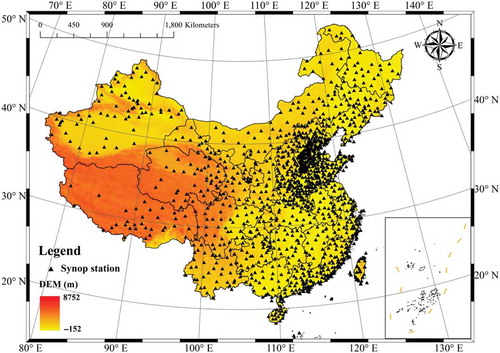
Table 1. Conversion table from octa to percentage units for TCCs (from China Meteorological Administration).

Unit	TCCs
Octas	0	1	2	3	4	5	6	7	8	9
Percentages (%)	0	10	25	40	50	60	75	90	100	Null

Usually, surface observations in China are conducted at 6-hour intervals, at 00:00, 06:00, 12:00, 18:00 Coordinated Universal Time (UTC). To ensure adequate Synop observations matched with satellite overpasses (around local time 13:30), only data at 06:00 UTC were used. In order to ensure that there are adequate samples for the comparison and considering the data availability of both Synop observations and satellite observations, the year 2009 was selected in this study. For all days in January, April, July, and October corresponding to winter, spring, summer, and autumn in 2009, TCCs at 06:00 UTC from all the available stations of China were collected for comparison.

2.2. TCCm

Aqua/MODIS cloud mask products (MYD35) were used to calculate the TCCm. We chose the latest version products (Collection 6.0). In this product, 11 bands were selected for cloud detection, and both infrared and visible techniques were applied for detecting different types of cloud (Ackerman et al. 1998, 2010). The cloud detection results are classified into four types: confident clear (, represents the confidence interval of clear), probably clear (), probably cloudy (), and confident cloudy (). This product is recognized as clear-conservative.

Here, we merged the probably clear and probably cloudy classes into the confident ones, so that the cloud mask images had only two classes: 1 representing cloudy and 0 representing clear. These MODIS cloud mask products were in swath projection with a spatial resolution of 1 km, and only every fifth pixel contained the geolocation information. Therefore, we used the geolocation products MYD03 to provide geographic coordinates for every 1 km pixel. MYD35 data over China within the time range of 05:30–06:30 UTC were selected to ensure that the time discrepancy between the two TCC data sets was less than 30 min, and the data within the same period of Synop observations were selected. The TCCm was calculated as the percentage of cloudy pixels within the same FOV of TCCs.

2.3. Auxiliary maps

For the significant difference case analysis, three auxiliary maps were used. Two of them are the Aqua/MODIS aerosol optical depths (AODs) at 550 nm derived from the Deep Blue and Dark Target algorithms. MODIS has been demonstrated to be capable of monitoring air pollution at various spatial scales (Chu et al. 2003). The Dark Target algorithm can retrieve the AOD over the vegetation land and ocean with gaps over bright surfaces such as deserts (Gautam et al. 2009). And the Deep Blue algorithm is able to distinguish dust plumes from fine-mode pollution (i.e. PM 2.5) particles even under complex aerosol conditions (Hsu et al. 2006). Thus, 1-degree daily MYD08 Collection 5.1 AOD 550 nm Deep Blue products in April (to characterize the dust storm regions) and Dark Target products in October (to characterize the air pollution regions) of 2009 were used. The two auxiliary maps are the monthly average AOD in April and October over China. Another map is the snow cover in January 2009. The 4 km daily Interactive Multisensor Snow and Ice Mapping System (IMS) snow cover products (Ramsay 1998) were used to calculate the monthly snow mask map in China (snow means there has been at least 1 day with snow cover, and no snow means the number of days with snow cover is zero). These products are often used for validation use of snow cover (Yang et al. 2014).

2.4. Intercomparison strategies

Before the comparison, we used a statistical method to estimate the average FOV with the highest occurrence frequency for the surface observations in China. This method starts by varying the satellite FOV from a radius of 5 to 200 km with an interval of 5 km, and then calculating the Pearson correlation coefficients between TCCs and TCCm. The average FOV is assumed to have the highest correlation coefficient in the comparison because when the satellite FOV is smaller or larger than the average FOV, more spatial differences will be introduced. After determining the average FOV for TCCs, the TCCm is calculated as the cloud fraction in the same FOV. For the comparison purpose, we used as displayed in Equation (1) to represent the difference between TCCs and TCCm, a positive indicates that Synop reports larger TCC than MODIS, while a negative indicates that Synop reports smaller TCC than MODIS.

(1)

3. Results and discussion

3.1. The determination of the average FOV

The correlation coefficients between TCCs and TCCm were calculated from all the instantaneous Synop and MODIS observations in four seasons of 2009. The number of pairs (N) for comparison was 9909, 11623, 9301, and 7630 over spring, summer, autumn, and winter, respectively. Figure 2 illustrates the correlation coefficients at different FOV radii varying from 5 to 200 km at an interval of 5 km. The general variation patterns of the correlation coefficients in the four seasons were very similar, all of which increased sharply from a small FOV and decreased gradually after reaching the peak region where we determined the average FOV. It is obvious that the correlation coefficient decreases when the FOV difference between Synop and MODIS becomes larger. The average correlation coefficient ranged from 0.644 in winter to 0.711 in summer.

Figure 2. Correlation coefficients (R) between TCCs and TCCm at different FOV radii. N represents the number of TCC pairs for comparison in each season.

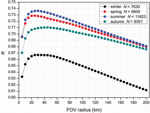
For each season, there was a significant peak region with high correlation coefficients indicating a good agreement between TCCs and TCCm. Outside the peak region, more differences were introduced by the spatial discrepancy between these two data sets. Therefore, we defined the peak region as the range of average FOVs for every season. As shown in Figure 2 and Table 2, we calculated correlation coefficients at FOV radius from 15 to 200 km at an interval of 5 km. As listed in Table 2, the highest correlation coefficient was 0.729, 0.736, 0.710, and 0.667 in the four seasons and the corresponding average FOV range was 20–25, 25–35, 35–50, and 25–45 km, respectively (shown in Table 2). Obviously, these four FOV ranges are close in value and overlapped with each other, which indicates that there is a relatively constant range for surface observation of cloud. Combining the four seasons, this range can be like a radius of 20 to 50 km. Additionally, with more complex atmospheric conditions, autumn and winter had a larger range of average FOV than spring and summer since the visible range of surface observers can be affected by different conditions.

Table 2. The correlation coefficients at the FOV radius from 15 to 55 km and the average FOV range for each season is marked in the grey region.

FOV radius (km)	15	20	25	30	35	40	45	50	55
Spring	0.726	0.729	0.729	0.728	0.727	0.726	0.725	0.723	0.722
Summer	0.731	0.735	0.736	0.736	0.736	0.735	0.733	0.732	0.731
Autumn	0.703	0.706	0.708	0.709	0.710	0.710	0.710	0.710	0.709
Winter	0.661	0.665	0.667	0.667	0.667	0.667	0.667	0.666	0.665

Actually, for each observation, the FOV may vary with different factors like the station elevation, cloud base height, and visibility. Thus, it is unable to set a FOV for each observation. For each season, the peak region indicates the FOVs with high occurrence frequency and R. Therefore, we used the average FOV for comparison purpose and defined it as 35 km in China for all the seasons. The value of 35 km was in the average FOV radius ranges of all the seasons except for spring but the difference in the correlation coefficient was merely 0.002, thus, this FOV radius was reasonable for the comparison in different seasons.

3.2. The influence of different FOVs on the comparison

As shown in Figure 2, the correlation coefficient at FOVs outside the peak region is relatively low, especially at extremely small or large FOV radii. The decrease in the correlation coefficient was mainly contributed by the spatial discrepancy between TCCs and TCCm. We extracted three satellite FOV radii of 5, 35, and 150 km in summer to analyse the influence of spatial discrepancy on the comparison. The satellite FOV at a radius of 35 km is equal to the surface average FOV, and is expected to be best matched in the spatial domain with Synop. The value of 5 km is much smaller than the average FOV radius, and the 150 km radius FOV almost covers the same area as the ISCCP regular grid (2.5° spatial resolution). MYD35 products at 1 km resolution make us capable of resampling TCC data at various resolutions larger than 1 km.

Figure 3 displays the distribution of at different TCCs (Synop) for the three satellite FOVs. For 5 km radius, the variation range of the difference at 2–5 octas is much larger than at 35 km, while a relatively smaller difference appears at 1 and 6–8 octas. For 150 km radius, the majority of the differences at 1–3 octas as well as the mean difference are out of the 25% range, and the variation ranges at 7 and 8 octas are obviously larger than that at 35 km. These results reveal that there is more difference under partly cloudy conditions when the satellite FOV is smaller than the average FOV, while there is more difference at extremely small or large TCC when it is larger than the average FOV.

Figure 3. The distribution of at different TCCs and the grey region indicates that the absolute difference is within 12.5% (nearly 1 octas). (a) FOV radius at 5 km, (b) FOV radius at 35 km, (c) FOV radius at 150 km. In the box plot, the range of each grey box is given as 25% to 75% percentile, and the middle line is given as 50% percentile. The black rectangle indicates the mean value.

3.3. Comparison between TCCs and TCCm

Based on the average FOV with a radius of 35 km, we conducted a detailed comparison between TCCs and TCCm. All the matched observations were used for analysis. The monthly mean TCCs is 74.78%, 74.41%, 66.5%, and 74.06% for each season (from spring to winter), and the corresponding TCCm is 75.27%, 78.34%, 73.82%, and 82.12%, respectively. At this monthly mean scale, the differences between TCCs and TCCm are relatively small (less than one octa, i.e. 12.5%), all being less than 10%, and for spring and summer they are even below 5%. Both in autumn and winter, TCCm is about 6% larger than TCCs, which suggests that MODIS reports more cloud than Synop. An important reason is that compared to surface observers, MODIS can detect more cirrus, which is hard for human eyes to identify.

Daily instantaneous TCCs and TCCm were also gathered for direct comparison, and the number of samples for comparison was 9909, 11623, 9301, and 7630 over the four seasons (from spring to winter). As shown in Table 3, the mean differences for all the seasons are negative values, of which spring has the smallest difference of −0.49% and winter has the largest of −8.07%, indicating that MODIS observed a greater TCC than the Synop. Since the mean difference at each season was calculated from thousands of instantaneous Synop and MODIS observations, the results of the mean differences prove a good agreement between TCCs and TCCm. The correlation is stronger in spring (0.727) and summer (0.736) than autumn (0.710) and winter (0.667). The root mean square error (RMSE) presents similar behaviour as the mean differences and correlation coefficients. It is slightly greater in autumn (26.84%) and winter (26.45%) than spring (24.08%) and summer (21.59%), all of which were around 25% (2 octas).

Table 3. Difference statistics for instantaneous TCCs and TCCm.

Season	Mean Dsm (%)	RMSE (%)	Correlation coefficient (R)	Number of observations (N)
Spring	−0.49	24.08	0.727	9909
Summer	−3.93	21.59	0.736	11623
Autumn	−7.33	26.84	0.710	9301
Winter	−8.07	26.45	0.667	7630

Table 4 illustrates how the differences are distributed at different TCC. For all the seasons, the greater differences occurred at small TCC (1–4 octas, equal to 10% to 50%). The disparity decreased to nearly 5% for TCC over 7 octas, which indicates that the two TCC data sets had better agreement at large TCC. This may be associated with specific cloud types, for example, when the sky is covered by some cirrus and surface observer reports little cloud, there may be large disparity between TCCs and TCCm. Spring and summer had lower differences than autumn and winter at 1–4 octas, especially at the small TCC. However, when the cloud cover exceeded that range, the differences for winter and autumn decreased sharply, and spring showed the highest difference at 6–8 octas. These results were in line with Figure 4 that autumn and winter tended to have greater difference at small TCC while spring had more difference at large TCC compared to other seasons.

Table 4. Mean difference between TCCs and TCCm at different TCCs, N represents the number of instantaneous observations.

Season octas	Mean Dsm (%)
	1	2	3	4	5	6	7	8
Spring	−10.3	−13.01	−9.78	−7	1.33	5.05	3.41	1.45
N	(845)	(884)	(313)	(319)	(422)	(902)	(3338)	(2886)
Summer	−10.14	−15.89	−12.13	−10.43	−6.78	−2.53	−1.06	0.66
N	(598)	(1114)	(493)	(428)	(610)	(1532)	(4640)	(2208)
Autumn	−20.11	−24.35	−18.92	−13.05	−5.77	−0.1	0.28	0.51
N	(1307)	(1201)	(407)	(335)	(402)	(838)	(2571)	(2240)
Winter	−29.66	−32.08	−22.7	−18.29	−11.9	−3.56	−1.41	1.14
N	(793)	(729)	(244)	(204)	(283)	(584)	(2114)	(2679)

Figure 4. The frequency distribution of differences () for four seasons: (a) spring, (b) summer, (c) autumn, (d) winter. The Gaussian fitting curve is added in each figure.

Figure 4 shows the frequency distribution of differences () for four seasons, together with the Gaussian fitter curve for each season. Samples of each season have passed the Kolmogorov−Smirnov normality test at the 0.05 level of significance. Over 60% of the differences were within the −10% to 10% range, which is less than 1 octa (Figure 4). The frequency of differences in this range was 65.53%, 63.85%, 60.81%, and 66.53%, respectively, from spring to winter. The TCCs is a series of discrete values of integral octa while TCCm is a real number, thus, when the TCC difference falls in the range from −1 to 1 octa, it indicates that the two TCC are consistent. There were some special features in different seasons. Unlike the other three seasons, summer has the highest frequency in the −10% to 0% range, which might due to the high occurrence frequency of cirrus in summer than in the other seasons since MODIS could detect more cirrus than the visual observation (Li et al. 2004). Spring had higher frequency in the range of 60−100% (frequency: 4.35%) than the other seasons. In contrast, autumn and winter had higher frequencies in the range of −100% to −60% (autumn frequency: 5.68%, winter frequency: 5.71%). These large differences suggested that there were significant inconsistences between TCCs and TCCm.

3.4. Significant difference case analysis

To analyse the cases with significant inconsistences between Synop and MODIS, we extracted instantaneous observations with absolute difference over 80%, which meant that TCCs and TCCm were in the opposite mode, one was cloud-free and the other was overcast. As suggested by Qian et al. (Qian et al. 2006), observations of cloud-free sky and overcast sky are more reliable than partly cloudy conditions. Therefore, in these significant cases, both Synop and MODIS have a high-level confidence reporting cloud-free or overcast. All the TCCs were either 0/1 octa or 7/8 octas, while all the TCCm were either 0–10% or 90–100%. The extracted significant difference cases in each season are shown in Figure 5.

Figure 5. Synop stations with significant difference cases, N represents the number of significant cases in each season: (a) spring, (b) summer, (c) autumn, (d) winter. The rad points represent that is above 80% and the blue points represent is below −80%. The auxiliary maps are AOD at 550 nm (Deep blue), AOD at 550 nm (Dark target) and snow cover for spring, autumn and winter respectively. The inset outlines the south China Sea Islands with dashed line representing the national boundary of China.

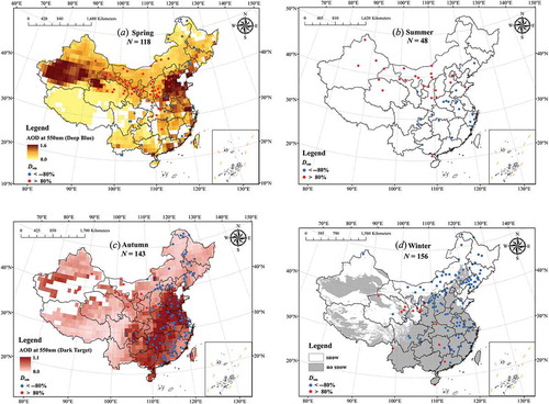
In spring, as shown in Figure 5(a), the significant differences mostly occurred in the northwest China, which is frequently hit by dust storms with relatively high AOD (Cyranoski 2003). However, the cases did not locate in the highest AOD regions like Xinjiang and Hebei Province but mostly in the northwest China such as the Hexi Corridor and the Loess Plateau. The spatial distribution of those cases is consistent with the spreading path of dust storms. We noticed that in these cases, TCCs reported large TCC while TCCm reported small TCC. An explanation for this phenomenon is that the floating dust aerosols might influence surface observations, the observers tend to misclassify dust as cloud and report large TCC. However, when a dust storm appears, TCCs will be recorded as 9 (an invalid value).

However, in autumn and winter as shown in Figures 5(c) and (d), the majority of these significant difference cases were Synop reporting cloud-free skies while the MODIS reported overcast skies. Some of them occurred in the northern and northeastern region (e.g. Heilongjiang, Jilin, Liaoning, and Inner Mongolia Province), where there would be snow when the temperature drops to rather low. It is obvious that winter had more such cases than autumn. MODIS was likely to misinterpret snow cover as cloud while the surface observations were less likely to confuse these two. This could also explain the −100% to −60% differences in autumn and winter since the snow cover would occupy a large area and change with time, resulting in large difference between TCCs and TCCm.

In addition to the snow cover influence, we also noticed that both in autumn and winter, significant difference cases occurred in North China Plain (NCP) and some eastern region (e.g. Hebei, Shandong, Shanxi, Henan, Jiangsu, Anhui, Hubei, Zhejiang, Fujian, Hunan, Guangdong, and Jiangxi Province). When compared with the AOD map, the spatial pattern of these cases is more obvious. The aerosol loading in these regions is larger than other regions and most of them suffer from the influence of haze, especially in autumn and winter (Wang et al. 2006; Kim et al. 2007; Cao et al. 2007). Haze is a combination of different fine-mode pollution particles, much smaller than dust. These haze-induced cases are very likely to mix with the snow-induced cases. Under such conditions, MODIS tended to overestimate TCC due to misclassification of haze as cloud, while surface observers tended to underestimate it because the obscuring effect of haze on thin and middle cloud (Warren, Eastman, and Hahn 2007). Therefore, TCCm was much larger than TCCs.

As illustrated in Figure 5, spring, autumn, and winter had more significant difference cases than summer (Figure 5(b)) since summer suffered less from the influence of dust, haze or snow. However, for the four seasons, the spatial distributions of those significant difference cases were very similar. The positive ones mostly occurred in the northwest China while the negative ones occurred in the NCP and east China.

4. Summary and looking forward

4.1. Spatio-temporal matching for the comparison

The comparison between TCCs and TCCm was based on accurate temporal-spatial matching because the two data sets differ both in observation time and geometry (or FOV). The matching process can ensure a good temporal-spatial consistency between TCCs and TCCm, and the comparison would directly reflect their different cloud observation ability and TCC accuracy. For the temporal matching, Kotarba et al. (Kotarba 2009) tested two time discrepancies, 30 min and 10 min, and the results obtained from these two were not significantly different, which indicates that the Synop data collected within 30 min before or after the MODIS overpass time can be used as a good approximation of exactly matched observations. Therefore, in this study, we applied this 30 min limit, and only MODIS data in the range of 05:30–06:30 were selected for comparison to match with Synop (at 06:00 UTC).

For the spatial matching, previous studies always used an empirical FOV with a radius of 30 km to characterize the surface observation FOV (Kotarba 2009; Sun et al. 2014; Fontana et al. 2013; Seiz, Foppa, and Walterspiel 2009). However, the FOV for each observation can be affected by many factors, such as the cloud height and type, the visible environment of Synop stations, and even the observation techniques of surface observers. Thus, instead of adopting this 30 km, we tested different FOV radii (from 5 to 200 km with an interval of 5 km) to estimate the average FOV with the highest occurrence frequency and R between TCCs and TCCm. The estimation was based on a large number of instantaneous observations (over 7000) for each season. As the results show, the radius range of average FOV in China is 20–25, 25–35, 35–50, and 25–45 km from spring to winter. It turns out that the FOV radius is in a range rather than a constant value, which verifies our assumption that it can be affected by many factors. In the range, the correlation coefficient for each FOV varies little, which indicates that the occurrence frequencies for the FOVs in the peak region are similar to each other. Subsequently, we conducted the FOV sensitivity test using three different FOV radii (5, 35, and 150 km) as to see how the spatial discrepancy between TCCs and TCCm would influence the comparison results. We concluded that when the satellite FOV is much smaller or larger than the surface average FOV, more differences would be introduced. For FOV radius like 5 and 150 km with low occurrence frequency, significant differences would be introduced. We also calculated the statistics shown in Table 3 for the FOV radius of 30 and 55 km, respectively (see Supplemental Table S1 at http://dx.doi.org/10.1080/01431161.2015.1072651). Compared to the results of 35 km radius, there is no big difference for 30 km radius, while R of 55 km radius is about 0.05 smaller than that of 35 km radius. Thus, we have experimentally verified that the traditional-used 30 km is also a reasonable radius for FOV over China.

4.2. The comparison between TCCs and TCCm

For the comparison purpose, we set the average FOV radius for China as 35 km. We found that at monthly mean scale, TCCs was 74.78%, 74.41%, 66.5%, and 74.06% for each season and the corresponding TCCm was 75.27%, 78.34%, 73.82%, and 82.12%. The monthly mean differences are much less than the daily difference, as suggested by Qian et al. (Qian et al. 2012). This can be explained by Figure 4 in which the frequency distribution of the differences in all seasons shows a normal distribution, thus, the frequency of positive values is quite close to the negative ones. When calculating the monthly mean, these two would offset each other. However, the daily instantaneous comparison is the basis for the monthly comparison and can clearly show the difference between TCCs and TCCm, especially those significant difference cases shown in Figure 5.

From the daily instantaneous comparison in each season in 2009, the correlation between TCCs and TCCm was stronger in spring (0.727) and summer (0.736) than in autumn (0.710) and winter (0.667). The number of samples used in this calculating was all over 7000. The mean differences (the difference was defined as TCCs minus TCCm) for all the seasons are negative values, indicating that MODIS reports more cloud than Synop. These overestimations can be explained by MODIS’s stronger ability to detect cirrus than Synop (Fontana et al. 2013; Kotarba 2009; Kästner, Bissolli, and Hoppner 2004). The frequency distribution of the differences showed that for all seasons over 60% of the differences were within the −10% to 10% range (less than 1 octa). The frequency of differences in this range was 65.53%, 63.85%, 60.81%, and 66.53%, respectively, from spring to winter. And we also noticed that for all seasons, the greater differences occurred at small TCC (1–4 octas). Therefore, from the view point of climate study which usually uses long-term TCC data over a big domain, we can conclude that these two TCC data sets have good agreement over China.

4.3. Analysis of significant difference cases

In addition to this comparison work between TCCs and TCCm over China, we also analysed the significant difference cases. And that is what is inspiring our future study. The significant difference cases have two important characters, one is that Synop and MODIS reported completely opposite TCC, and the other is that both TCC have a high level of confidence. Using the summer with a relative smaller number of cases as a reference, we found that the spatial distribution of those cases in the four seasons had an obvious pattern and matched well with the underlying maps. It is interesting that for these four seasons, there were dominant factors controlling the occurrence of those cases. For spring and autumn, it was the aerosol loading as the AOD maps show. However, the aerosol types in these two seasons are different, for spring it is dust aerosol in northwest China while for autumn it is haze in NCP and some eastern areas. It seems that different aerosols have different effects on Synop and MODIS observations. The dust aerosol tends to obscure Synop observations resulting in larger TCCs, while the haze mainly results in smaller TCCs and larger TCCm. For winter, the dominant factor was snow cover, as most of the cases matched well with the snow cover map. In these cases, the MODIS turned to misinterpret snow as cloud and Synop did not have such a problem.

In future study, we will use more accurate TCC records (like the lidar data) to validate those cases as to clarify the right one between TCCs and TCCm, especially in spring and autumn. And since we have recognized that the aerosol types and concentration may influence the Synop observations, it is urgent for us to figure out whether the long-time TCCs have been affected by them. China would be our perfect study area because it suffers from serious air pollution, providing a good environment for use in the study of the effect of aerosols on cloud observations.

Disclosure statement

No potential conflict of interest was reported by the authors.

Supplemental data

Supplemental data for this article can be accessed at http://dx.doi.org/10.1080/01431161.2015.1072651.

Acknowledgements

Dr Zhanqing Li, Dr Arthur Cracknell, and Pauline Lovell are greatly acknowledged for their valuable suggestions and supports. The surface cloud observation data were obtained from China Meteorological Administration (CMA). MODIS products were downloaded from NASA website. IMS data were provided by the National Snow & Ice Data Center (NSIDC). The computation of this work was supported by Tsinghua National Laboratory for Information Science and Technology.

ORCID

Hui Lu http://orcid.org/0000-0003-1640-239X

Additional information

Funding

This work was jointly supported by the National Basic Research Program of China [2015CB953703], the National Natural Science Foundation of China [51190092, 41371328 and 51109111], the National ‘863’ Program of China [2012AA12A309], Tsinghua University Initiative Research Program [2011081132], and the Beijing Higher Education Young Elite Teacher Project [YETP0132].

References

- Ackerman, S., K. Strabala, P. Menzel, R. Frey, C. Moeller, and L. Gumley. 2010. “Discriminating Clear-Sky from Cloud with MODIS Algorithm Theoretical Basis Document (MOD35).” In Paper presented at the MODIS Cloud Mask Team, Cooperative Institute for Meteorological Satellite Studies. Madison: University of Wisconsin.
- Ackerman, S. A., K. I. Strabala, W. Paul Menzel, R. A. Frey, C. C. Moeller, and L. E. Gumley. 1998. “Discriminating Clear Sky from Clouds with MODIS.” Journal of Geophysical Research: Atmospheres (1984–2012) 103 (D24): 32141–32157. doi:10.1029/1998JD200032.
- Barrett, E. C., and C. K. Grant. 1979. “Relations between Frequency Distributions of Cloud over the United Kingdom Based on Conventional Observations and Imagery from LANDSAT 2.” Weather 34 (11): 416–424.
- Cao, J. J., S. C. Lee, J. C. Chow, J. G. Watson, K. F. Ho, R. J. Zhang, Z. D. Jin, Z. X. Shen, G. C. Chen, Y. M. Kang, S. C. Zou, L. Z. Zhang, S. H. Qi, M. H. Dai, Y. Cheng, and K. Hu. 2007. “Spatial and Seasonal Distributions of Carbonaceous Aerosols over China.” Journal of Geophysical Research-Atmospheres 112: D22S11. doi:10.1029/2006jd008205.
- Chu, D. A., Y. J. Kaufman, G. Zibordi, J. D. Chern, J. Mao, C. Li, and B. N. Holben. 2003. “Global Monitoring of Air Pollution over Land from the Earth Observing System‐Terra Moderate Resolution Imaging Spectroradiometer (MODIS).” Journal of Geophysical Research: Atmospheres (1984–2012) 108 (D21): 4661.
- Cyranoski, D. 2003. “China Plans Clean Sweep on Dust Storms.” Nature 421 (6919): 101. doi:10.1038/421101a.
- Fontana, F., D. Lugrin, G. Seiz, M. Meier, and N. Foppa. 2013. “Intercomparison of Satellite- and Ground-Based Cloud Fraction over Switzerland (2000–2012).” Atmospheric Research 128: 1–12. doi:10.1016/j.atmosres.2013.01.013.
- Gautam, R., Z. Liu, R. P. Singh, and N. Christina Hsu. 2009. “Two Contrasting Dust‐Dominant Periods over India Observed from MODIS and CALIPSO Data.” Geophysical Research Letters 36: 6. doi:10.1029/2008GL036967.
- Hahn, C. J., W. B. Rossow, and S. G. Warren. 2001. “ISCCP Cloud Properties Associated with Standard Cloud Types Identified in Individual Surface Observations.” Journal of Climate 14 (1): 11–28.
- Hsu, N. C., S.-C. Tsay, M. D. King, and J. R. Herman. 2006. “Deep Blue Retrievals of Asian Aerosol Properties during Ace-Asia.” IEEE Transactions on Geoscience and Remote Sensing 44 (11): 3180–3195. doi:10.1109/TGRS.2006.879540.
- Jovanovic, B., D. Collins, K. Braganza, D. Jakob, and D. A. Jones. 2011. “A High-Quality Monthly Total Cloud Amount Dataset for Australia.” Climatic Change 108 (3): 485–517. doi:10.1007/s10584-010-9992-5.
- Kahn, B. H., M. T. Chahine, G. L. Stephens, G. G. Mace, R. T. Marchand, Z. Wang, C. D. Barnet, A. Eldering, R. E. Holz, R. E. Kuehn, and D. G. Vane. 2008. “Cloud Type Comparisons of AIRS, Cloudsat, and CALIPSO Cloud Height and Amount.” Atmospheric Chemistry and Physics 8 (5): 1231–1248. doi:10.5194/acp-8-1231-2008.
- Kaiser, D. P. 1998. “Analysis of Total Cloud Amount over China, 1951–1994.” Geophysical Research Letters 25 (19): 3599–3602. doi:10.1029/98GL52784.
- Kästner, M., P. Bissolli, and K. Hoppner. 2004. “Comparison of a Satellite Based Alpine Cloud Climatology with Observations of Synoptic Stations.” Meteorologische Zeitschrift 13 (3): 233–243. doi:10.1127/0941-2948/2004/0013-0233.
- Kazantzidis, A., P. Tzoumanikas, A. F. Bais, S. Fotopoulos, and G. Economou. 2012. “Cloud Detection and Classification with the Use of Whole-Sky Ground-Based Images.” Atmospheric Research 113: 80–88. doi:10.1016/j.atmosres.2012.05.005.
- Kim, S.-W., S.-C. Yoon, J. Kim, and S.-Y. Kim. 2007. “Seasonal and Monthly Variations of Columnar Aerosol Optical Properties over East Asia Determined from Multi-Year MODIS, LIDAR, and AERONET Sun/Sky Radiometer Measurements.” Atmospheric Environment 41 (8): 1634–1651. doi:10.1016/j.atmosenv.2006.10.044.
- Kotarba, A. Z. 2009. “A Comparison of Modis-Derived Cloud Amount with Visual Surface Observations.” Atmospheric Research 92 (4): 522–530. doi:10.1016/j.atmosres.2009.02.001.
- Li, Y., R. Yu, Y. Xu, and X. Zhang. 2004. “Spatial Distribution and Seasonal Variation of Cloud over China Based on ISCCP Data and Surface Observations.” Journal of the Meteorological Society of Japan 82 (2): 761–773. doi:10.2151/jmsj.2004.761.
- Ma, J. J., H. Wu, C. Wang, X. Zhang, Z. Q. Li, and X. H. Wang. 2014. “Multiyear Satellite and Surface Observations of Cloud Fraction over China.” Journal of Geophysical Research: Atmospheres 119 (12): 7655–7666. doi:10.1002/2013jd021413.
- Meerkötter, R., C. König, P. Bissolli, G. Gesell, and H. Mannstein. 2004. “A 14‐Year European Cloud Climatology from NOAA/AVHRR Data in Comparison to Surface Observations.” Geophysical Research Letters 31 (15): L15103. doi:10.1029/2004GL020098.
- Pavolonis, M. J., and A. K. Heidinger. 2005. “Preliminary Global Cloud Comparisons from the AVHRR, MODIS, and GLAS: Cloud Amount and Cloud Overlap.” In Paper presented at the Fourth International Asia-Pacific Environmental Remote Sensing Symposium 2004: Remote Sensing of the Atmosphere, Ocean, Environment, and Space. Honolulu, HI: SPIE.
- Qian, Y., D. P. Kaiser, L. Ruby Leung, and M. Xu. 2006. “More Frequent Cloud‐Free Sky and Less Surface Solar Radiation in China from 1955 to 2000.” Geophysical Research Letters 33: 1.
- Qian, Y., C. N. Long, H. Wang, J. M. Comstock, S. A. McFarlane, and S. Xie. 2012. “Evaluation of Cloud Fraction and Its Radiative Effect Simulated by IPCC AR4 Global Models against ARM Surface Observations.” Atmospheric Chemistry and Physics 12 (4): 1785–1810. doi:10.5194/acp-12-1785-2012.
- Ramsay, B. H. 1998. “The Interactive Multisensor Snow and Ice Mapping System.” Hydrological Processes 12 (10–11): 1537–1546. doi:10.1002/(ISSN)1099-1085.
- Rossow, W. B., and R. A. Schiffer. 1991. “ISCCP Cloud Data Products.” Bulletin of the American Meteorological Society 72 (1): 2–20. doi:10.1175/1520-0477(1991)072<0002:ICDP>2.0.CO;2.
- Rossow, W. B., A. W. Walker, and L. C. Garder. 1993. “Comparison of ISCCP and Other Cloud Amounts.” Journal of Climate 6 (12): 2394–2418. doi:10.1175/1520-0442(1993)006<2394:COIAOC>2.0.CO;2.
- Salomonson, V. V., W. Barnes, P. W. Maymon, H. E. Montgomery, and H. Ostrow. 1989. “MODIS: Advanced Facility Instrument for Studies of the Earth as a System.” IEEE Transactions on Geoscience and Remote Sensing 27 (2): 145–153. doi:10.1109/36.20292.
- Seiz, G., N. Foppa, and J. Walterspiel. 2009. “Use of Satellite-Based Products within the National Climate Observing System (GCOS Switzerland).” Paper presented at the Proceedings of the EUMETSAT Meteorological Satellite Conference, Bath, September 21–25.
- Sun, L., X. Xia, P. Wang, and Y. Fei. 2014. “Do Aerosols Impact Ground Observation of Total Cloud Cover over the North China Plain?” Global and Planetary Change 117: 91–95. doi:10.1016/j.gloplacha.2014.03.009.
- Taylor, P. C. 2012. “Tropical Outgoing Longwave Radiation and Longwave Cloud Forcing Diurnal Cycles from CERES.” Journal of the Atmospheric Sciences 69 (12): 3652–3669. doi:10.1175/JAS-D-12-088.1.
- Thomas, S. M., A. K. Heidinger, and M. J. Pavolonis. 2004. “Comparison of Noaa’s Operational Avhrr-Derived Cloud Amount to Other Satellite-Derived Cloud Climatologies.” Journal of Climate 17 (24): 4805–4822.
- Wang, G. H., K. Kawamura, S. Lee, K. F. Ho, and J. J. Cao. 2006. “Molecular, Seasonal, and Spatial Distributions of Organic Aerosols from Fourteen Chinese Cities.” Environmental Science & Technology 40 (15): 4619–4625. doi:10.1021/Es060291x.
- Warren, S. G., R. M. Eastman, and C. J. Hahn. 2007. “A Survey of Changes in Cloud Cover and Cloud Types over Land from Surface Observations, 1971-96.” Journal of Climate 20 (4): 717–738. doi:10.1175/JCLI4031.1.
- Xiong, X., and W. Barnes. 2006. “An Overview of MODIS Radiometric Calibration and Characterization.” Advances in Atmospheric Sciences 23 (1): 69–79. doi:10.1007/s00376-006-0008-3.
- Yang, J., L. Jiang, J. Shi, S. Wu, R. Sun, and H. Yang. 2014. “Monitoring Snow Cover Using Chinese Meteorological Satellite Data over China.” Remote Sensing of Environment 143: 192–203.
- Zhang, Y. W., H. Lu, and J. Cai. 2014. “Towards the Comparison of Satellite and Ground Based Cloud Amount over China.” Remote Sensing of the Atmosphere, Clouds, and Precipitation V 9259. doi:10.1117/12.2068979.