Urban population estimation based on residential buildings volume using IKONOS-2 images and lidar data

ABSTRACT

This paper presents a methodological approach to estimation of urban population using the volume of single houses and high-rise residential buildings obtained from an IKONOS-2 ortho-image and light detection and raging (lidar) data. The estimates are directly executed at the finest scale level (i.e. the housing unit) and are then aggregated at the census district level for further validation with the aid of official data supplied by the local and federal governments. Unlike prior works, this study executes a thorough assessment of horizontal and elevation accuracy for the IKONOS-2 and lidar data used in the experiment. The methodological stages are threefold: the construction of a 3D city model, the accuracy assessment of the ortho-image and digital surface models (DSMs), and the quantification of urban population. The validation was accomplished by means of linear regression and associated hypothesis tests, considering the estimated population and the reference data. The results showed that there was a systematic underestimation of population. On average, the conducted estimates assessed 31 fewer inhabitants per district and lie 1.35% below the expected values given by the reference data. In spite of the observed underestimation, the estimated population can be regarded as equivalent to the population provided by the reference data at a 1% level of significance.

1. Introduction

Cities in developing countries keep on growing in a rapid and uncontrolled way. In order to support public actions related to the monitoring of and interventions in the urban environment, targeted at providing its inhabitants with fair and balanced access to housing, social infrastructure, public transportation, sanitation, and other public services, it is essential to have updated information on the dynamics of both urban and demographic growth. The knowledge of how many people live in a certain geographic area or political-administrative unit is valuable information, especially for local planning initiatives (National Research Council [US] and Mapping Science Committee 2002).

In this way, population estimates have become a major area of concern in view of their importance for public policies and land management. In recent decades, inter-census population counts have not been undertaken on a regular basis in developing countries, thus depriving federal, state, and local governments of up-to-date information on their respective population contingents. Meanwhile, the ever-increasing growth of urban populations in such countries impacts cities’ infrastructure and social equipment, demanding greater efficiency and responsiveness of public authorities in the planning and management of urban resources. These scenarios of sudden demographic changes render crucial for local government the access of authorities to precise information on the real dimensions of urban population and its spatial distribution (Henderson and Xia 1997).

Remote-sensing data have been used for the purpose of assessing human settlements surfaces and population density at several scales since the late 1970s and early 1980s. Some works were exclusively based on aerial photography (Vining and Louw 1978; Lo and Chan 1980; Olorunfemi 1982), some were based on optical data (Lo and Welch 1977; Henderson 1979; Iisaka and Hegedua 1982; Jensen et al. 1983), while others employed synthetic aperture radar (SAR) data (Henderson and Anuta 1980; Lo 1986a, 1986b; Melia and Sobrino 1987). At this early stage of research, population estimates mostly relied on simple methods, like linear regression models and allometric functions.

Advances in digital image processing techniques, in parallel with the emergence of new imaging satellites from the late 1980s and early 1990s onwards, represented a new boost for studies in this field in the following decades, and hence, research using satellite imagery for population estimates dealing with innovative methods and sensors has become more widespread (Langford and Unwinn 1994; Henderson 1995; Lo 1995; Henderson and Xia 1997; Harvey 2002; Faure et al. 2003; Lo 2005; Wu, Qiu, and Wang 2005; Wu and Murray 2007; Hoque 2008). Such methods include dasymetric mapping and kernel techniques to build population density surfaces. The use of texture and contextual measures, such as urban pixel density, homogeneity, entropy, and distance from the city centre, associated with housing densities by means of linear regression models, has also been explored (Webster 1996). Additional studies based on texture were carried out by Chen (2002), Souza (2003), Li and Weng (2005), Liu, Clarke, and Herold (2006), and Wu, Qiu, and Wang (2006) among others.

Night-time satellite imagery has also been used worldwide for estimating population density, such as in the USA (Sutton et al. 1997; Anderson et al. 2010), in China (Lo 2001), in Brazil (Amaral et al. 2006), and in Europe (Briggs et al. 2007). Sutton et al. (1997) derived night-time stable light imagery from the visible near-infrared band of 231 orbits of the Defence Meteorological Satellite Program Operational Linescan System (DMSP-OLS (ordinary least squares)). Analyses of the saturated areas of the images indicated strong correlations between the areas of saturated clusters and populations in those areas. Radiance-calibrated DMSP-OLS data were also used, to evaluate their potential for population estimation in China at the provincial, county, and city levels (Lo 2001). The author dealt with linear regression models, regarding the Chinese population and population density as the dependent variable, and the light area, light volume, and pixel mean as independent variables. It was found that the DMSP-OLS night-time data produced reasonably accurate estimates of urban population using either the light area or light volume as input. The total sums of the estimates for both urban and total population closely approximated the true values given by Chinese statistics at all three spatial levels.

Further experiments dealing with innovative methods have included the use of interpolation (Xie 2006; Reibel and Agrawal 2007) or refined dasymetric maps (Langford 2006; Briggs et al. 2007; Azar et al. 2010; Kim and Yao 2010), and more advanced techniques, such as residual kriging (Liu, Kyriakidis, and Goodchild 2008), geographically weighted regression (GWR; Lo 2008), sub-pixel analysis (Lu, Weng, and Li 2006; Wu and Murray 2007; Azar et al. 2010), GWR coupled with sub-pixel analysis (Joseph, Wang, and Wang 2012), geographical information system (GIS) data for spatially refined analyses (Qiu, Woller, and Briggs 2003; Reibel 2007; Deng, Wu, and Wang 2010), and cellular automata (Zhan, Silva, and Santillana 2010), to mention only a few examples. More recent works have also started regularly to introduce very-high-resolution (VHR) images for assessing population spatial distribution and density. In this regard, Liu, Clarke, and Herold (2006) investigated the correlation between census population density and IKONOS-2 image texture. The spatial unit adopted for the analysis was census blocks with homogeneous land use. The image texture was described using three methods: the grey-level co-occurrence matrix (GLCM), semi-variance, and spatial metrics. The authors suggest that the correlation is not strong enough to predict or forecast residential population, but the image texture from the VHR images does provide a base with which to refine census-reported population distribution using remote sensing. Similar studies include the use of IKONOS-2 and QuickBird images for identifying homogeneous residential zones (Souza 2003; Almeida et al. 2007), IKONOS-2 images and GIS for assessing population density (Yagoub 2006), as well as time-series of QuickBird imagery and ancillary data for investigating sub-tribal populations and population dynamics (Stofan 2008; Lang et al. 2010).

The advent of optical very high-spatial resolution sensors with stereo capabilities and airborne laser scanners has opened the way for a new generation of population estimation studies which include the third dimension in their quantitative analyses, making use of buildings volume data extracted from height models. Xie (2006) interpolated population at the lowest spatial level (housing unit) by means of a dasymetric map, allocating population counts to each unit with the aid of DOQQ (digital orthophoto quarter quads), light detection and raging (lidar) data from the ALTM (Airborne Laser Terrain Mapper) 1233 sensor, and parcel data. Other work in this field concerns the use of a deterministic model for population estimation at the sub-block level using GIS building data and census housing statistics (Wu, Wang, and Qiu 2008). These two works, however, did not generate lidar 3D models per se, but rather imported it from a GIS database. Lwin and Murayama (2009) proposed a methodological framework for employing volumetric information derived from lidar data, although such elevation data were not in fact been used in their research. Almeida et al. (2011) carried out deterministic population estimation for an informal settlement comprising both single and multi-family dwellings, but as opposed to the former works, they used a height model extracted from a stereo-pair of IKONOS-2 images. In a more recent paper, Wang (2013) proposed the creation of indices related to the area or volume of residential buildings based on VHR imagery and lidar in order to enable the indirect estimation of population, which was further cross-validated with official census data.

Qiu, Sridharan, and Chun (2010) explored the use of building volumes derived from lidar as a population indicator by means of a probabilistic model. In addition to an OLS regression model, they adopted a spatial autoregressive model to account for the spatial autocorrelation in the regression residuals, significantly increasing the goodness-of-fit of the volume-based estimates conducted at the block level. Another probabilistic model was conducted by Lu et al. (2010), using QuickBird imagery and lidar data for estimating population at the census block level for an area mostly occupied by single houses. Further probabilistic models were elaborated by Dong, Ramesh, and Nepali (2010) and Silván-Cárdenas et al. (2010). In the former work, the authors built GWR and OLS regression models based on lidar, Landsat Thematic Mapper (LS/TM), and parcel data sets, considering building count, area, and volume, and in all cases underestimations were observed at the census block level. In the latter work, likewise the former, building count, area, and volume were also used for comparison among seven OLS regression models based on lidar data and aerial photography, which indicated that a simple model taking into account residential building counts alone provided the most reliable population estimates. More recently, Sridharan (2011) employed an expectation maximization (EM) algorithm to disaggregate the census block-level population into individual residential buildings based on their volume obtained from lidar data. This author then conceived an initial regression model between the building-level population and the volume, in which the EM algorithm was again used to iteratively refine the regression parameters by minimizing the residuals of the re-aggregated block-level population, achieving a more accurate representation of the residential population distribution.

The present work is based on a PhD dissertation (Tomás 2010) published by the National Institute for Space Research (INPE). The added novel value of this article to the dissertation concerns a comprehensive and updated literature review, as well as a thorough revision of the set of equations related to population estimation, to ensure that each step of the calculation is clearly understandable by the reader. This study integrates the last generation of population estimates studies and reports a deterministic method for estimating population using buildings footprints extracted from IKONOS-2 images and ALTM 2025 lidar-derived building volumes, in a study area intensively occupied by high-rise residential buildings. The estimates are directly executed at the finest-scale level (i.e. the housing unit) and are then aggregated at the census district level for further validation with the aid of official data supplied by the local and federal governments. Unlike prior works, this study executes a thorough assessment of elevation accuracy for the lidar data used in the population estimation experiment.

2. Study area

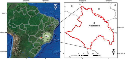
The selected study area is a central sector of Uberlândia city, seat of Uberlândia municipality, located in the southeastern state of Minas Gerais, Brazil (Figure 1). The city is located 550 km from Belo Horizonte, the state capital, and its initial point has the coordinates 18º 55ʹ 07ʺ S and 48º 16ʹ 38ʺ W. According to the last demographic census in 2010 (IBGE 2010), the municipality had a population of 604,013 inhabitants (146.78 inhabitants/km²).

Figure 1. Location of Uberlândia municipality.

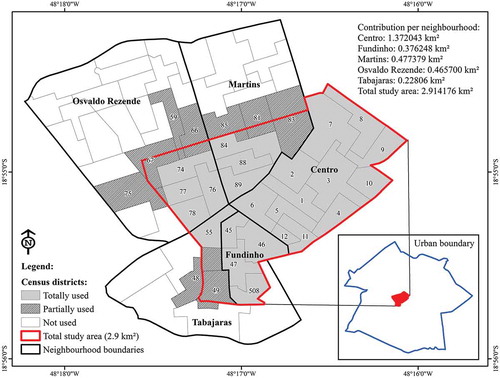
The city itself is located on a mildly undulated terrain, with a mean altitude of 1000 m above sea level and it presents a hot and tropical climate, with a mean annual rainfall of 1500 mm and an average temperature of 22ºC. The occupation patterns of its central neighbourhoods are very diverse, consisting of green areas, one- and two-storey buildings, as well as clusters of high-rise residential and business buildings. The study area entirely comprises the neighbourhoods Centro and Fundinho as well as part of Tabajaras, Martins, and Osvaldo Rezende neighbourhoods (Figure 2).

Figure 2. Study area boundaries (in red) and urban boundary of the Uberlândia municipality seat (in blue) in the inset.

3. Methodology

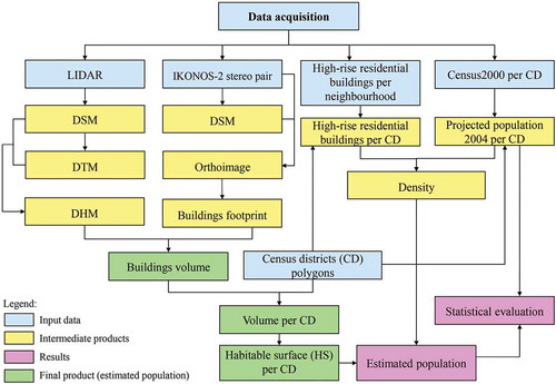
The methodology is summarized in Figure 3 and it includes three main stages: (1) the 3D model construction, (2) accuracy assessment of the ortho-image and the digital surface models (DSMs), and (3) population estimates. The construction of the 3D model can be subdivided into two sub-steps: extraction of buildings footprints in an ortho-image derived from an IKONOS-2 stereo-pair and processing of lidar data.

Figure 3. Methodology flowchart.

3.1. Construction of the 3D model

3.1.1. Preprocessing of IKONOS-2 images for the extraction of buildings footprints

Initially, two IKONOS-2 images with 11 bits of radiometric resolution were used for generating a DSM intended to orthorectify one of the images, namely that with the smallest viewing angle. Table 1 shows the main characteristics of the IKONOS-2 stereo-pair.

Table 1. Main characteristics of the IKONOS-2 stereo-pair.

Acquisition date	27 June 2008	27 June 2008
Position in the stereo-pair	Left	Right
Sensor elevation angle (°)	60.84	81.80
Sensor azimuth angle (°)	27.17	117.45
Solar azimuth angle (°)	32.76	32.55
Solar elevation angle (°)	40.55	40.66

For both IKONOS-2 image sets (left and right), the four multispectral bands of 4.0 m spatial resolution were pan-sharpened with the panchromatic band with 1.0 m of resolution using the Gram–Schmidt method (Laben and Brower 2000) in ENVI 4.8.

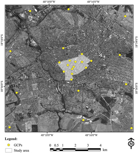
In order to collect ground control points (GCPs) for generating the DSM, field work was executed aiming at identifying remarkable features regularly scattered over the study area. In total, 54 GCPs were acquired with a differential global positioning system (GPS) in static mode, of which 25 were used for DSM generation and the remaining 29 for accuracy assessment as independent checkpoints (ICPs).

The GCPs were inserted in both stereo-pair images (Figure 4) using PCI Geomatica OrthoEngine software to allow the creation of epipolar images with the rational function model (RFM), followed by the generation and geocoding of the DSM at 1.0 m spatial resolution, enabling further orthorectification of the right stereo-pair image, since this has the smallest viewing angle (8.2°). The extraction of buildings footprints was finally performed in this ortho-image.

Figure 4. Location of GCPs in the right-hand image of the IKONOS-2 stereo-pair.

3.1.2. Laser scanning data acquisition and processing

The laser scanning was accomplished with the sensor ALTM 2025 (Airborne Laser Terrain Mapper) produced by Optech Inc. This airborne survey, carried out between 2 February and 18 June 2004, adopted Marégrafo de Imbituba/SC as the elevation datum, SAD-69 (South American Datum 1969) as the horizontal datum, and UTM (Universal Transverse Mercator) – Fuse 22 – K-Zone as the cartographic projection system, with a scanner frequency of 33 Hz, a laser repetition rate of 25,000 Hz, and a viewing angle of 12°.

The acquired lidar data were preprocessed and delivered in ASCII (American Standard Code for Information Interchange) format, containing the information of the x, y, and z coordinates as well as the intensity of the DSM. A filtering process was applied to the DSM to obtain the digital terrain model (DTM), while the TerraScan module, available with the software Terra Solid, was employed to this end.

TerraScan collects an irregularly spaced 3D points cloud and, by means of its terrain classifier, known as Axelsson’s progressive triangular irregular network (TIN) densification algorithm (Axelsson 1999, 2000), it extracts points directly located on the terrain surface by constructing an iterative TIN. This algorithm initiates by selecting the parameter ‘building maximum size’.

If, for instance, this parameter is 60 m, the software assumes that any area within 60 m × 60 m will have at least one point on the terrain and that the lowest point belongs to the terrain. In this work, this parameter was set to 85 m.

Axelsson’s algorithm initially builds a TIN considering the points with the lowest elevation. The triangle faces of the initial TIN are mostly situated below the terrain, and only their vertices make contact. The algorithm then starts moving the TIN upwards through the iterative addition of new points belonging to the cloud to the network. Each newly added point brings the TIN increasingly closer to the terrain. According to Axelsson (1999, 2000), an advantage of this algorithm is its ability to handle discontinuous surfaces – particularly useful in urban areas.

The iteration parameters determine how close a point should be to a triangle face in order to be acknowledged as a point belonging to the terrain and be added to the TIN. The iteration angle is one of such parameters and it is defined as the maximum angle between a given point, its projection on the closest triangle face, and the vertex of the closest triangle. The iteration distance parameter, in turn, assures that there will be no abrupt jump to the next iteration in the case of large triangles. This is what enables the inclusion of small buildings in the model. The smaller the iteration angle, the less sensitive the algorithm will be in detecting changes in the points cloud (small undulations in the terrain or points located on vegetation of reduced height). According to the software producer, TerraSolid (2010), it is recommended to use a small angle (close to 4º) in flat areas and a wider angle (approximately 10º) in steeper areas.

It is possible to correct errors where the automatic classification (filtering process) does not yield good results, through the command ‘add point to the terrain’. Based on this classification result, two files in the text file (TXT) format were generated: one containing the DSM and the other the DTM. These TXT files were imported in ArcGIS 9.3 for the generation of surfaces, according to Patenaude et al. (2004). The DSM points cloud was also converted in a TIN in ArcGIS, and both TINs (DSM and DTM) were then converted to a regular grid by means of Delaunay triangulation. This conversion procedure yielded the DSM and DTM files actually employed for population estimation.

3.2. Accuracy assessment of the data employed for population estimation

The accuracy standards in Brazil are ruled by the Cartographic Accuracy Standard – CAS (Padrão de Exatidão Cartográfica – PEC), which determines that horizontal accuracy is defined as a function of the scale module (denominator), and elevation accuracy as a function of the equidistance between contour lines. As noted in Brazil (1984), 90% of the points related to remarkable features in an image, when cross-checked in terms of their actual position on the terrain, must not present an error greater than that established by PEC. In the same way, 90% of scattered elevation points obtained by the interpolation of contour lines, when tested on the terrain, must not present an error greater than that established by PEC.

PEC is a statistical indicator of dispersion related to 90% probability, which defines the accuracy of cartographic products. This 90% probability corresponds to 1.6449 times the standard error (SE), and isolated errors in a cartographic product must not exceed 60.8% of PEC.

The root mean square error (RMSE) is given by:

(1) $\mathrm{R}\mathrm{M}\mathrm{S}\mathrm{E}=\sqrt{ \frac{1}{n}\sum _{i=1}^n\mathrm{\Delta }{\mathrm{\Omega }}_i^2},$(1)

where $\mathrm{\Omega }$ corresponds to the horizontal components (E and N) in the case of the ortho-image accuracy assessment, and to elevation (h) in the case of the DSM accuracy assessment; n is the number of evaluated points.

According to Brazil (1984), cartographic products are ranked as a function of their accuracy as belonging to classes A, B, and C, as shown in Table 2.

Table 2. Cartographic accuracy standard (PEC).

Map	Horizontal		Elevation
	PEC	Standard error	PEC	Standard error
Class A	0.5 mm $\times$ Scale†	0.3 mm $\times$ Scale†	1/2 $\times$ Equidistance	1/3 $\times$ Equidistance
Class B	0.8 mm $\times$ Scale†	0.5 mm $\times$ Scale†	3/5 $\times$ Equidistance	2/5 $\times$ Equidistance
Class C	1.0 mm $\times$ Scale†	0.6 mm $\times$ Scale†	3/4 $\times$ Equidistance	1/2 $\times$ Equidistance

† Scale module.

Source: Brazil, 1984.

In order to fulfil these requirements, it is necessary to conduct a statistical evaluation taking into account the discrepancies between the coordinates of points belonging to the cartographic product under analysis and those of homologous points obtained by field survey, provided that these two sets of data lie within the same cartographic projection system and both have the same horizontal and elevation datum.

As previously stated, accuracy tests are specifically based on a 10% level of statistical significance and they comprise both trend and accuracy analyses.

3.2.1 Trend analysis

According to Galo and Camargo (1994), trend analysis is based on a statistical analysis of discrepancies between the observed coordinates in the cartographic product and the reference coordinates, calculated for each sample point, i as:

(2) $\mathrm{\Delta }{X}_i=X_i-X_i^{\mathrm{r}},$(2)

where X_i are the calculated values and $X_i^{\mathrm{r}}$ are the reference values.

The mean and standard deviation of the sampling differences are respectively calculated as:

(3) $\mathrm{\Delta }\bar{X}=\frac{1}{n} \sum _{i=1}^n\mathrm{\Delta }{X}_i,$(3)

and

(4) $S_{\mathrm{\Delta }X}= \sqrt{\frac{1}{n-1} \sum _{i=1}^n{(\mathrm{\Delta }{X}_i-\mathrm{\Delta }\bar{X})}^2},$(4)

where $\mathrm{\Delta }\bar{X}$ is the mean and $S_{\mathrm{\Delta }X}$ is the standard deviation of the sampling discrepancies.

In the trend tests, the following hypotheses are evaluated:

(5) $H_0:\mathrm{\Delta }\bar{X}=0\left(\mathrm{n}\mathrm{u}\mathrm{l}\mathrm{l}\mathrm{h}\mathrm{y}\mathrm{p}\mathrm{o}\mathrm{t}\mathrm{h}\mathrm{e}\mathrm{s}\mathrm{i}\mathrm{s}\right),\mathrm{a}\mathrm{g}\mathrm{a}\mathrm{i}\mathrm{n}\mathrm{s}\mathrm{t}$(5)

(6) $H_1:\mathrm{\Delta }\bar{X}\ne 0\left(\mathrm{a}\mathrm{l}\mathrm{t}\mathrm{e}\mathrm{r}\mathrm{n}\mathrm{a}\mathrm{t}\mathrm{i}\mathrm{v}\mathrm{e}\mathrm{h}\mathrm{y}\mathrm{p}\mathrm{o}\mathrm{t}\mathrm{h}\mathrm{e}\mathrm{s}\mathrm{i}\mathrm{s}\right).$(6)

In this test, the sample t-statistics (t_sample) must be calculated in order to check whether its value lies within the interval for accepting or refusing the null hypothesis.

The value of the sample t-statistics is calculated as:

(7) $t_X=\frac{\mathrm{\Delta }\bar{X}}{S_{\mathrm{\Delta }X}}\sqrt{n},$(7)

and the confidence interval as:

(8) $\left|t_X\right|<t_{\left(n-1;\alpha /2\right),}$(8)

where n is the sample size (i.e. the number of individuals in a sample), n – 1 is the number of degrees of freedom, and α is the level of significance, set as 5% in this work.

If the sample t-statistics lie beyond the confidence interval, the null hypothesis is rejected (i.e. the cartographic product must not be regarded as free of meaningful trends in the evaluated coordinate for the given significance level (Galo and Camargo 1994)). The presence of trends in any direction indicates the occurrence of a problem (which may have many causes), but once the cause is identified, its effect can be minimized by the subtraction of its value in each coordinate of the cartographic product (Galo and Camargo 1994).

3.2.2 Accuracy analysis

The accuracy analysis, in turn, concerns the comparison of the standard deviation related to the discrepancies with the expected standard deviation for the desired class by means of a hypothesis test. This test is formulated as follows:

(9) $H_0:S_{\mathrm{\Delta }X}={\sigma }_X,\mathrm{a}\mathrm{g}\mathrm{a}\mathrm{i}\mathrm{n}\mathrm{s}\mathrm{t}$(9)

(10) $H_1:S_{\mathrm{\Delta }X}>{\sigma }_X,$(10)

where ${\sigma }_X$ is the expected standard deviation for the class of interest.

Once the sample variance (square of the sample standard deviation – $S_{\mathrm{\Delta }X}^2$) is calculated, the chi-square statistics can be computed as:

(11) ${\chi }_X^2=\left(n-1\right)\frac{S_{\mathrm{\Delta }X}^2}{{\sigma }_X^2},$(11)

and we then verify whether its value lies within the interval of acceptance, as follows:

(12) ${\chi }_X^{ 2}{\le }_{\left(n-1;\alpha \right)}^{ 2}.$(12)

If the above expression is not fulfilled, the null hypothesis H₀ is rejected and the cartographic product is regarded as not up to the pre-established accuracy standard.

3.2.3 Sampling in cartographic accuracy assessment

A sound accuracy assessment procedure depends on the number of points used. In this way, it is not possible to have a limited number of points, in which case one cannot assure the assessment is reliable; neither is an excessive number of points possible, for which the analysis is reliable but the costs are unfeasible (Nogueira Júnior 2003).

For Merchant (1982), the accuracy of a map at a small scale (1:20,000 or less) must be assessed with a minimum number of 20 points well defined both in the map and on the terrain (homologous points), the latter being related, for instance, to street intersections or boundaries of real estate properties.

The size of a sample refers to the amount of unities or individuals within a given area which are actually considered for analysis. It is known that samples selection must occur on a random basis, to avoid any bias in the sampling procedure. By determining an appropriate sample size, it is possible to reduce costs and time in the analysis while simultaneously increasing data reliability (Nogueira Júnior 2003).

3.2.4 Accuracy assessment of the IKONOS-2 ortho-image

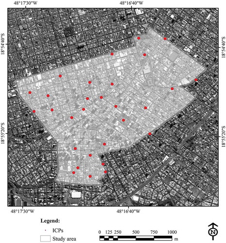
To assess the accuracy of the IKONOS-2 ortho-image, 29 ICPs were selected, all located on clearly identifiable sites in the scene. It is worth mentioning that none of these ICPs were used in the orthorectification process, in order not to introduce trend errors to the accuracy assessment. Figure 5 shows the location of the ICPs in the right-hand image of the IKONOS-2 stereo-pair.

Figure 5. Location of the ICPs in the right-hand image of the IKONOS-2 stereo-pair.

Based on the methodological approach proposed by Galo and Camargo (1994), the discrepancies in terms of UTM-WGS84 (World Geodetic System) coordinates (E, N) were calculated for each ICP, considering the values extracted from the ortho-image and the reference values, which are those obtained by the GPS equipment. It is worth remembering that, prior to the orthorectification stage, the ellipsoidal or geometric heights (related to the ellipsoid) derived from the GPS survey were converted to orthometric heights, which are those related to geoid or the mean sea level. To this end, it is necessary to know the geoidal height or undulation, namely the difference between the two reference surfaces – geoid and ellipsoid (Arana 2000).

Following the calculation of the coordinate discrepancies between the ortho-image and GPS data, we calculated the mean and standard deviation of the sample points (ICPs) discrepancies, the sample t-statistics and their respective confidence interval, the expected standard deviation and the confidence interval for the hypothesis test, the chi-square test, and the RMSE.

3.2.5 Accuracy assessment of the IKONOS-2 and lidar 3D models

Although the DSM generated with the IKONOS-2 stereo-pair was not employed for population estimation, it was statistically evaluated since it had been applied in the orthorectification of the stereo-pair right-hand image, which was in turn further used for extracting buildings footprints.

The accuracy assessment for both DSMs, namely that derived from the IKONOS-2 stereo-pair and the lidar DSM, was performed by calculating the elevation discrepancies for each ICP, considering the GPS data as reference values. As with accuracy assessment of the ortho-image, evaluation of the DSMs involved the same statistical tests.

3.3 Extraction of buildings footprints

The buildings footprints were extracted from the IKONOS-2 ortho-image by digitizing the buildings boundaries on the screen. Since not all buildings are residential, it was necessary to discriminate such buildings from those related to commercial and services use (office towers, hotels, and commercial activities). Considering that this type of information cannot be obtained by remotely sensed data and or was not available at the cadastre of the local government of Uberlândia, fieldwork was undertaken in order to identify the uses of all buildings within the study area.

3.4 Population estimation

In order to make use of the 3D information rendered available by the DSM, it was necessary to generate a DTM and then subtract this from the DSM to obtain the digital height model (DHM), which accounts for the volume effectively utilized for residential use. The DHM was superimposed onto the residential buildings footprints layer (in vector format), and by taking into account the height for each residential building provided by the DHM, the residential buildings volume was calculated by multiplying the area of each footprint by the corresponding building height (Equation (13)). This calculation was aggregated at the census district (CD) level, given the fact that the reference data for the population estimates were available at this level of analysis:

(13) $\mathrm{R}\mathrm{B}{\mathrm{V}}_{\mathrm{C}\mathrm{D}}=\sum _{i=1}^n(\mathrm{R}\mathrm{B}\mathrm{A}{)}_{i }\times {\left(\mathrm{R}\mathrm{B}\mathrm{H}\right)}_i,$(13)

where RBV_CD corresponds to the total residential building volume of a CD, RBA_i to the ith residential building area, RBH_i to the ith residential building height, and n denotes the total number of residential buildings found in the considered CD.

According to a method proposed by Almeida et al. (2011), the population estimates were realized based on the calculation of the habitable surface (HS). The HS (Figure 6) of an ith residential building is given by the ratio of the ith residential building volume (RBV_i) to the average height from floor to ceiling ($\overline{\mathrm{D}\mathrm{F}\mathrm{C}}$), as in Equation (14):

(14) $\mathrm{H}{\mathrm{S}}_i= {\left(\mathrm{R}\mathrm{B}\mathrm{V}\right)}_{i }/ \left(\overline{\mathrm{D}\mathrm{F}\mathrm{C}}\right),$(14)

Figure 6. Example of HS_i calculation.

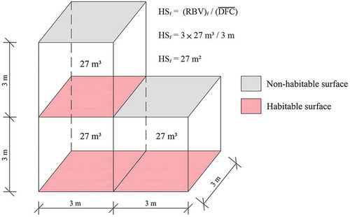
where $\overline{\mathrm{D}\mathrm{F}\mathrm{C}}$ is set to 3 m.

For estimation of residential population at the CD level in 2004 ($\mathrm{E}\mathrm{R}{\mathrm{P}}_{\mathrm{C}\mathrm{D}2004}$), the aggregated value of HS per district (HS_CD2004) was multiplied by a population density factor, also determined at the district level ($\mathrm{P}{\mathrm{D}}_{\mathrm{C}\mathrm{D}2004}$):

(15) $\mathrm{E}\mathrm{R}{\mathrm{P}}_{\mathrm{C}\mathrm{D}2004}= {\left(\mathrm{H}\mathrm{S}\right)}_{\mathrm{C}\mathrm{D}2004} \times {\left(\mathrm{P}\mathrm{D}\right)}_{\mathrm{C}\mathrm{D}2004}.$(15)

In order to assess the population density in each CD, we initially calculated a proportional area ratio (PAR_CD) derived from the division of the surface of each district effectively included in the study area of this work (SISA_CD) by the district total area (TA_CD):

(16) $\mathrm{P}\mathrm{A}{\mathrm{R}}_{\mathrm{C}\mathrm{D}}= {\left(\mathrm{S}\mathrm{I}\mathrm{S}\mathrm{A}\right)}_{\mathrm{C}\mathrm{D}}/(\mathrm{T}\mathrm{A}{)}_{\mathrm{C}\mathrm{D}}.$(16)

This proportional ratio was respectively applied to the total number of inhabitants living in each district according to the 2000 census (CP_CD2000), so as to provide the proportional population in 2000 (PP_CD2000):

(17) $\mathrm{P}{\mathrm{P}}_{\mathrm{C}\mathrm{D}2000}= {\left(\mathrm{P}\mathrm{A}\mathrm{R}\right)}_{\mathrm{C}\mathrm{D}} \times {\left(\mathrm{C}\mathrm{P}\right)}_{\mathrm{C}\mathrm{D}2000}.$(17)

The values for TA_CD, PAR_CD, CP_CD2000, and PP_CD2000 are shown in Table 3. The proportional population at the district level for the reference year 2000 (PP_CD2000) was then further employed for determining the proportional projected population for the year of the study (2004). The Brazilian Institute of Geography and Statistics (IBGE) provides population yearly estimates at the neighbourhood level for all Brazilian municipalities. We generated a population growth rate at the neighbourhood level (PGR_NG) by dividing the IBGE neighbourhood population estimated in 2004 (EP_NG2004) by the neighbourhood census population in 2000 (CP_NG2000) (Table 4). Since a neighbourhood comprises several districts (see the first two columns of Table 3), this rate remained constant for all districts belonging to the same neighbourhood:

(18) $\mathrm{P}\mathrm{G}{\mathrm{R}}_{\mathrm{N}\mathrm{G}}= {\left(\mathrm{E}\mathrm{P}\right)}_{\mathrm{N}\mathrm{G}2004}/(\mathrm{C}\mathrm{P}{)}_{\mathrm{N}\mathrm{G}2000}.$(18)

Table 3. Population data at the census district (CD) level in 2000 and 2004.

CD code	Neighbourhood	TACD (m^2)	SISACD (m^2)	PARCD (dimens.) †	CPCD2000 (inh.) ‡	PPCD2000 (inh.) ‡	PGRNG (dimens.) †	PPPCD2004 (inh.) ‡
1	Centro	102,793	102,793	1.0000	467	467	1.1372	531
2	Centro	119,251	119,251	1.0000	544	544		619
3	Centro	206,860	206,860	1.0000	553	553		629
4	Centro	87,350	87,350	1.0000	531	531		604
5	Centro	74,233	74,233	1.0000	590	590		671
6	Centro	119,400	119,400	1.0000	622	622		707
7	Centro	237,772	237,772	1.0000	586	586		666
8	Centro	136,408	136,408	1.0000	638	638		726
9	Centro	103,120	103,120	1.0000	779	779		886
10	Centro	87,851	87,851	1.0000	626	626		712
11	Centro	66,600	66,600	1.0000	464	464		528
12	Centro	30,405	30,405	1.0000	642	642		730
Sub-total	Centro	1,372,043	1,372,043	1.0000	7,042	7,042		8,009
45	Fundinho	59,856	59,856	1.0000	638	638	1.1369	725
46	Fundinho	130,909	130,909	1.0000	659	659		749
47	Fundinho	103,970	103,970	1.0000	661	661		751
508	Fundinho	81,513	81,513	1.0000	788	788		896
Sub-total	Fundinho	376,248	376,248	1.0000	2,746	2,746		3,121
81	Martins	98,952	29,468	0.2978	638	190	1.1372	217
83	Martins	211,154	119,049	0.5638	619	349		397
84	Martins	131,006	131,006	1.0000	633	633		720
85	Martins	102,621	13,956	0.1360	860	117		133
88	Martins	81,005	81,005	1.0000	796	796		905
89	Martins	102,895	102,895	1.0000	709	709		806
Sub-total	Martins	727,633	477,379	0.6561	4,255	2,794		3,178
59	Osvaldo Rezende	83,322	6,574	0.0789	798	63	1.1373	72
66	Osvaldo Rezende	114,732	28,568	0.2490	763	190		216
67	Osvaldo Rezende	132,186	61,850	0.4679	624	292		332
74	Osvaldo Rezende	104,418	104,418	1.0000	722	722		821
75	Osvaldo Rezende	170,981	11,080	0.0648	802	52		59
76	Osvaldo Rezende	96,203	96,203	1.0000	804	804		914
77	Osvaldo Rezende	71,777	71,777	1.0000	760	760		864
78	Osvaldo Rezende	85,230	85,230	1.0000	838	838		953
Sub-total	Osvaldo Rezende	858,849	465,700	0.5422	6,111	3,721		4,231
48	Tabajaras	121,762	46,367	0.3808	856	326	1.1368	371
49	Tabajaras	102,539	86,471	0.8433	651	549		624
55	Tabajaras	89,968	89,968	1.0000	631	631		717
Sub-total	Tabajaras	314,269	222,806	0.7090	2,138	1,506		1,712
Total		3,649,042	2,914,176	0.7986	22,292	17,809	–	20,251

† dimens. = dimensionless

‡ inh. = number of inhabitants.

Table 4. Population and growth rate between 2000 and 2004.

Neighbourhood	Census population (CPNG2000) (inh.) †	Estimated population (EPNG2004) (inh.) †	Population growth rate (PGRNG) (dimensionless)
Centro	7,042	8,008	1.1372
Fundinho	2,746	3,122	1.1369
Martins	9,264	10,535	1.1372
Osvaldo Rezende	19,947	22,686	1.1373
Tabajaras	6,295	7,156	1.1368
Total	45,294	51,507	1.1372

Source: IBGE 2000; 2007.

† inh. = number of inhabitants.

The proportional projected population for the year 2004 at the district level (PPP_CD2004) resulted from the multiplication of the proportional population in 2000 (PP_CD2000) by the corresponding population growth rate at the neighbourhood level, as shown in Equation (19). The values for PPP_CD2004 are presented in the last column of Table 3:

(19) $\mathrm{P}\mathrm{P}{\mathrm{P}}_{\mathrm{C}\mathrm{D}2004}= {\left(\mathrm{P}\mathrm{P}\right)}_{\mathrm{C}\mathrm{D}2000} \times {\left(\mathrm{P}\mathrm{G}\mathrm{R}\right)}_{\mathrm{N}\mathrm{G}}.$(19)

PPP_CD2004 was used as our reference data. For our estimation in this work, we extracted PD_CD2004 by dividing PPP_CD2004 by the total residential area of each CD in 2004 (RA_{CD 2004}), as in Equation (20):

(20) $\mathrm{P}{\mathrm{D}}_{\mathrm{C}\mathrm{D}2004}={\left(\mathrm{P}\mathrm{P}\mathrm{P}\right)}_{\mathrm{C}\mathrm{D}2004}/{\left(\mathrm{R}\mathrm{A}\right)}_{\mathrm{C}\mathrm{D}2004}.$(20)

The total residential area of the CDs in 2004 was obtained by summing the dwellings surface data for each district, rendered available at the local real estate cadastre of the Uberlândia Planning Secretariat (PMU 2009). This cadastre, solely comprising information on residential real estate properties, consisted of a matrix and a map where the former contained a field associated with the city block code, which indicated on the map whether the block was within the study area limits or not.

3.4.1 Population estimation validation

In order to validate the estimated residential population, we compared our results to the population reference data through a simple linear regression given by:

(21) $Y_i={\beta }_0+{\beta }_1{X}_i+{\epsilon }_i,$(21)

where $Y_i$ is the population reference data (provided by IBGE) for the ith CD; $X_i$ is the estimated population (result of this work) for the ith CD; ${\beta }_0$ is the intercept; ${\beta }_1$ is the angular coefficient; and ${\epsilon }_i$ is the random error term, with E(ε_i) = 0 e σ²(ε_i) = σ².

We expect that the reference population and that estimated in this work be equivalent, and thus we assume that β₀ is equal to zero (β₀ = 0) and β₁ is equal to 1 (β₁ ≠ 0; β₁ = 1). These hypotheses are tested using Student’s t-test (Neter et al. 1996).

4. Results and discussion

4.1. IKONOS-2 DSM and ortho-image

IKONOS-2 DSM validation was accomplished by calculating the elevation discrepancy (h) of each ICP in relation to the corresponding points on the DSM. Based on these values, statistical measures such as mean, standard deviation, and RMSE, among others, were extracted as shown in Table 5. Although the DSM shows a trend, it met the accuracy standard for Class A at a scale of 1:10,000 according to PEC, and was further used to generate the ortho-image.

Table 5. Statistical results of the IKONOS-2 DSM validation.

Standard error (m)	1.67
Mean (bias) (m)	−11.24
Min error (m)	−4.51
Max error (m)	−13. 30
t (sample)	36.28
t (20;5%)	1.70
No trend	False
Chi-square (Class A – Scale 1:10,000)	28.06
Chi-square (20;5%)	37.92
DSM meets the accuracy standard 1:10,000 CLASSE A	True
RMSE (m)	1.67
PEC	2.74

In regard to positional accuracy, the IKONOS-2 ortho-image was validated by calculating the discrepancies between the east (E) and north (N) components of the ICPs and the corresponding E and N components associated with points found in the ortho-image. The results of the statistical tests show that both components, E and N, and their respective resultant present no trend and have an accuracy compatible with Class A at a scale of 1:2000 (Table 6).

Table 6. Statistical results of IKONOS-2 ortho-image validation.

	ΔE	ΔN	Resultant vector†
Standard error (m)	0.43	0.44	0.62
Mean (m)	−0.03	0.05	0.06
RMSE (m)	0.43	0.44	0.62
Trend analysis
tX	0.31	0.61	0.49
t (n-1; α/2)	1.70	1.70	1.70
| tX | < t (n-1; α/2)	True	True	True
Accuracy analysis – Class A
σX (1:2,000 – Class A)	0.42	0.42	0.60
${\chi }_X^{ 2}$	28.57	30.26	29.41
${\chi }_{\left(n-1;\alpha \right)}^2$	37.92	37.92	37.92
${\chi }_X^{ 2}$ ≤ ${ }_{\left(n-1;\alpha \right)}^{ 2}$	True	True	True

†Resultant vector is the sum of horizontal components E and N.

4.2. Lidar DSM and DTM

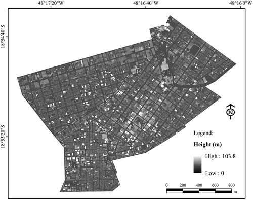
Lidar DSM and DTM (Figure 7) were validated by means of 42 ICPs, which like the GCPs were located at easily identifiable sites and evenly distributed throughout the scene. As mentioned in Section 3.3, the subtraction between these two products yielded the digital height model (DHM), as shown in Figure 8.

Figure 7. (a) DSM and (b) DTM generated using lidar data.

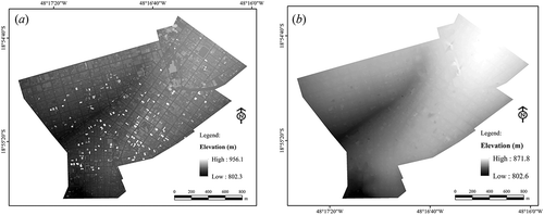
Figure 8. Digital height model (DHM).

Using the elevation discrepancies, we calculated the mean, standard deviation, and RMSE for both DSM and DTM. The value obtained for RMSE is meaningful for both DSM and DTM, denoting problems regarding trend, what indicates systematic error. The results in Table 7 show that the comparison between the sample t-value and the reference value reveals the presence of a trend in the H direction of both DSM and DTM. Such systematic influence in the H coordinate can be compensated by adding the mean value of this influence range with the inverted sign $(\hat{\mu }=-0,41)$in this coordinate, to reduce discrepancy.

Table 7. Statistical results of lidar DSM and DTM validation.

Statistics of elevation discrepancies
	DSM	DTM
Standard error (m)	0.25	0.25
Mean (m)	0.41	0.48
RMSE (m)	0.48	0.47
Trend analysis
n (number of points)	42	42
$\mathrm{\Delta }\bar{X}$ (m)	0.41	0.49
$S_{\mathrm{\Delta }X}$ (m)	0.25	0.24
Standard error 1:5,000 (m)	0.67	0.67
σX (m)	0.67	0.67
t (41; 0.05)	1.68	1.68
tX	10.73	3.03
Analysis	| tX | > tsample	| tX | > tsample
Component h	Trend observed	Trend observed
Accuracy analysis
n (number of points)	42	42
${\chi }_{\left(41;0.10\right)}^{ 2}$	52.95	52.95
$S_{\mathrm{\Delta }X}$ (m)	0.25	0.24
σX (m)	0.33	16.67
${\chi }_{\mathrm{X}(\mathrm{C}\mathrm{l}\mathrm{a}\mathrm{s}\mathrm{s}\mathrm{A})}^2$	22.38	0.01
Analysis	${\chi }_{X\left(\mathrm{C}\mathrm{l}\mathrm{a}\mathrm{s}\mathrm{s}\mathrm{A}\right)}^{ 2}$ < ${\chi }_{\left(41;0.10\right)}^{ 2}$	${\chi }_{X\left(\mathrm{C}\mathrm{l}\mathrm{a}\mathrm{s}\mathrm{s}\mathrm{A}\right)}^{ 2}$ < ${\chi }_{\left(41;0.10\right)}^{ 2}$
Scale to be used	1:5,000	1:5,000

Both DSM and DTM meet Class A standard at a 1:5000 scale (Table 7), although their usage must include certain restrictions in view of the calculated trend. In spite of this, the DHM obtained from the subtraction between DSM and DTM was employed to calculate the residential volume in this work.

4.3. Population estimation

Tables 8 and 9 present the proportional projected population (PPP_CD2004), the total residential area (RA_CD2004), the population density (PD_CD2004), the residential building volume (RBV), the habitable surface (HS_CD2004), and the estimated residential population (ERP_CD2004) per CD, grouped according to the neighbourhoods to which they belong. The number of decimal places for dimensionless measures (e.g. population density, population growth rate) was set at five, to avoid losing important differential information on the one hand and also not to produce coarse results on the other, ultimately aiming at generating sound estimates. All data related to surface and volume, including those obtained in the statistical tests, considered metric precision in regard to IKONOS and lidar data accuracy. The discrepancy between the estimated and reference data at the CD level is shown in Table 10.

Table 8. Calculation of population density, using the proportional projected population and total residential area.

Neighbourhood	Census district code	PPPCD2004 (inh.) †	Total residential area (m^2) (RACD2004)	Population density ($\mathrm{P}{\mathrm{D}}_{\mathrm{C}\mathrm{D}2004}$) (inh./m^2) †
Centro	1	531	50,475	0.01052
	2	619	49,919	0.01240
	3	629	45,845	0.01372
	4	604	39,426	0.01532
	5	671	50,988	0.01316
	6	707	84,874	0.00833
	7	666	46,541	0.01431
	8	726	39,011	0.01861
	9	886	44,058	0.02011
	10	712	54,268	0.01312
	11	528	42,927	0.01230
	12	730	64,374	0.01134
	Sub-total	8,009	612,706	0.01307
Fundinho	45	725	56,952	0.01273
	46	749	83,130	0.00901
	47	751	51,158	0.01468
	508	896	37,086	0.02416
	Sub-total	3,121	228,326	0.01367
Martins	81	217	6,995	0.03102
	83	397	12,627	0.03144
	84	720	37,915	0.01899
	85	133	762	0.17454
	88	905	52,464	0.01725
	89	806	62,048	0.01299
	Sub-total	3,178	172,811	0.01839
Osvaldo Rezende	59	72	3,706	0.01943
	66	216	3,229	0.06689
	67	332	10,600	0.03132
	74	821	45,636	0.01799
	75	59	1,614	0.03656
	76	914	49,008	0.01865
	77	864	58,856	0.01468
	78	953	53,240	0.01790
	Sub-total	4,231	225,889	0.01873
Tabajaras	48	371	73,320	0.00506
	49	624	37,704	0.01655
	55	717	57,590	0.01245
	Sub-total	1,712	168,614	0.01015
Total		20,251	1,408,346	0.01438

Table 9. Residential volume, habitable surface, population density, and estimated population per census district in 2004.

Neighbourhood	Census district code	Residential volume (m^3) (RBVCD)	$\overline{\mathrm{D}\mathrm{F}\mathrm{C}}$(m) ‡	Habitable surface (m^2) (HSCD2004)	Population density ($\mathrm{P}{\mathrm{D}}_{\mathrm{C}\mathrm{D}2004}$) (inh./m^2) †	Estimated residential population ($\mathrm{E}\mathrm{R}{\mathrm{P}}_{\mathrm{C}\mathrm{D}2004}$) (inh.) †
Centro	1	151,198	3.0	50,399	0.01052	530
	2	142,334		47,445	0.01240	588
	3	142,824		47,608	0.01372	653
	4	112,402		37,467	0.01532	574
	5	145,492		48,497	0.01316	638
	6	250,051		83,350	0.00833	694
	7	128,300		42,767	0.01431	612
	8	118,954		39,651	0.01861	738
	9	134,703		44,901	0.02011	903
	10	157,041		52,347	0.01312	687
	11	124,105		41,368	0.01230	509
	12	183,813		61,271	0.01134	695
	Sub-total	1,791,217		597,071	0.01307	7,821
Fundinho	45	177,198	3.0	59,066	0.01273	752
	46	238,071		79,357	0.00901	715
	47	162,673		54,224	0.01468	796
	508	105,163		35,054	0.02416	847
	Sub-total	683,105		227,701	0.01367	3,110
Martins	81	18,280	3.0	6,093	0.03102	189
	83	35,120		11,707	0.03144	368
	84	118,351		39,450	0.01899	749
	85	1,684		561	0.17454	98
	88	164,153		54,718	0.01725	944
	89	184,350		61,450	0.01299	798
	Sub-total	521,938		173,979	0.01839	3,146
Osvaldo Rezende	59	10,651	3.0	3,550	0.01943	69
	66	8,655		2,885	0.06689	193
	67	25,958		8,653	0.03132	271
	74	132,424		44,141	0.01799	794
	75	7,056		2,352	0.03656	86
	76	154,564		51,521	0.01865	961
	77	174,781		58,260	0.01468	855
	78	165,621		55,207	0.01790	988
	Sub-total	679,710		226,569	0.01873	4,217
Tabajaras	48	238,280	3.0	79,427	0.00506	402
	49	105,288		35,096	0.01655	581
	55	168,444		56,148	0.01245	699
	Sub-total	512,012		170,671	0.01015	1,682
Total		4,187,982	3.0	1,395,991	0.01438	19,976

† inh. = number of inhabitants.

‡ $\overline{\mathrm{D}\mathrm{F}\mathrm{C}}$ = average height from floor to ceiling

Table 10. Discrepancies between estimated and reference population data.

Neighbourhood	Census district code	Estimated residential population (ERPCD2004)	Reference data (PPPCD2004)	Discrepancies
Centro	1	530	531	−1
	2	588	619	−31
	3	653	629	24
	4	574	604	−30
	5	638	671	−33
	6	694	707	−13
	7	612	666	−54
	8	738	726	12
	9	903	886	17
	10	687	712	−25
	11	509	528	−19
	12	695	730	−35
	Sub-total	7,821	8,009	−188
Fundinho	45	752	725	27
	46	715	749	−34
	47	796	751	45
	508	847	896	−49
	Sub-total	3,110	3,121	−11
Martins	81	189	217	−28
	83	368	397	−29
	84	749	720	29
	85	98	133	−35
	88	944	905	39
	89	798	806	−8
	Sub-total	3,146	3,178	−32
Osvaldo Rezende	59	69	72	−3
	66	193	216	−23
	67	271	332	−61
	74	794	821	−27
	75	86	59	27
	76	961	914	47
	77	855	864	−9
	78	988	953	35
	Sub-total	4,217	4,231	−14
Tabajaras	48	402	371	31
	49	581	624	−43
	55	699	717	−18
	Sub-total	1,682	1,712	−30
Total		19,976	20,251	−275

Figure 9 shows the linear regression performed in regard to the estimated and reference population data, revealing a good fit for this model (R² = 0.99; t = 47.8; p < 0.01).

Figure 9. Linear regression for estimated and reference population data.

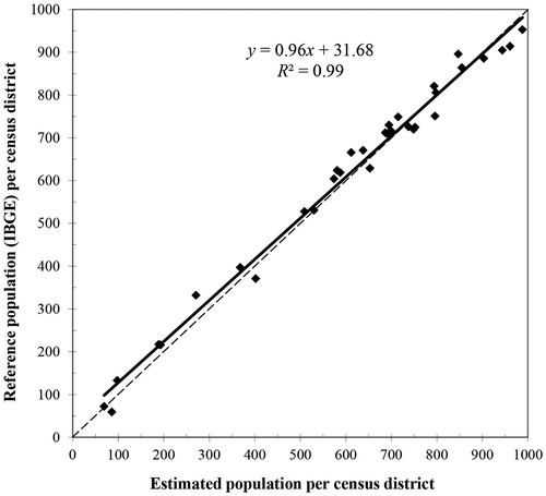
The t-test indicated that β₁ = 1 (t = –1.92; p = 0.06) and β₀ ≠ 0 (t = 2.39; p = 0.02) at a significance level of 5%. The estimated population presented on average 31 inhabitants fewer than the reference data. The discrepancies between the reference and estimated data reveal a systematic underestimation in our calculations, as shown in Table 10 and Figure 9. The total estimated population (19,976 inhabitants) for the study area is 1.36% fewer than the reference population (20,251 inhabitants). This trend is also observed at the neighbourhood level. However, when analysing such discrepancies individually (per CD), neither a positive nor negative variation in these values is observed (Table 10).

This underestimation can be explained by uncertainties introduced when resampling the reference data, originally available at the neighbourhood level, to the CD level, as well as by inconsistencies in the cadastral data provided by the Uberlândia Planning Secretariat. Despite such underestimation, the estimated data can be considered equivalent to the reference data at a significance level of 1%.

5. Conclusions

The goal of this research was to develop a methodological approach to estimate urban population using remote-sensing technologies. This approach was applied to central neighbourhoods in the municipality of Uberlândia, located in the state of Minas Gerais, southeastern Brazil. Lidar data were used in a model intended to incorporate information on building height, and thereby to refine population estimation.

Although the models obtained from lidar (DSM, DTM, DHM) proved to have satisfactory elevation accuracy, the imprecision in visually delimiting footprints posed some difficulties for building extraction. It was observed that the combination of spectral information obtained from orbital images with lidar was important for the interpretation and identification of features of interest. Hence, we suggest the use of images and height information obtained from lidar to improve assessment of buildings volume. Despite the availability of data with high horizontal and elevation accuracy such as IKONOS-2 images and lidar data, it is often not possible to identify residential buildings using only the spectral information, size, texture, or height of such targets. In the particular case of this work, it was necessary to carry out fieldwork to obtain this information, since it was not available in the local real estate cadastre of Uberlândia.

The lack of population estimates at the CD level for 2004 (the year of analysis) introduced uncertainties in the data used as reference, since we calculated the population growth rate per neighbourhood in order to obtain the reference values at the CD level. The comparison between population estimates and reference data showed that the former were underestimated by 1.36%. This underestimation can primarily be explained by the accumulation of uncertainties in reference data generation, as explained above. Nevertheless, the population estimates can be considered statistically equivalent to the reference data provided by the IBGE at a 1% level of significance.

The population estimates method proposed in this work is simple and can be potentially explored for monitoring the growth of urban population in densely occupied areas, to overcome the lack of updated data in inter-census periods. The method can support the planning and implementing of interventions in the urban space in response to social demands, provide basic information to local stakeholders and decision makers in the formulation of public policies, and supply information for demographic studies more precisely than those obtained from 2D data.

As a direction for future work, we intend to explore the classification of the lidar points cloud, aiming to identify buildings footprints in a more precise manner, thereby automating the extraction of the relevant polygons. We believe this would provide refined, and hence more accurate, results.

Acknowledgements

We thank Esteio Engineering and Survey Company S.A. for the donation of lidar data used in this article, and the Municipality of Uberlândia for providing the cadastral data to perform this work. Finally, the authors thank the anonymous reviewers for considerably improving the final quality of this paper.

Disclosure statement

No potential conflict of interest was reported by the authors.

Additional information

Funding

We gratefully acknowledge the financial support granted to this research by the Brazilian Institute for Space Research – INPE and the Brazilian Coordination for the Upgrade of Graduate Personnel – CAPES.

References

- Almeida, C. M., C. G. Oliveira, C. D. Rennó, and R. Q. Feitosa. 2011. “Population Estimates in Informal Settlements Using Object-Based Image Analysis and 3D Modeling.” ICEO-IEEE Earthzine, August 16. Accessed 24 February 2013. http://www.earthzine.org/2011/08/16/population-estimates-in-informal-settlements-using-object-based image analysis-and-3d-modeling/
- Almeida, C. M., I. M. Souza, C. D. Alves, C. M. D. Pinho, M. N. Pereira, and R. Q. Feitosa. 2007. “Multilevel Object-Oriented Classification of Quickbird Images for Urban Population Estimates.” In: Proceedings of the 15th ACM International Symposium on Advances in Geographic Information Systems (ACM GIS 2007), Miami: University of Florida. doi:10.1145/1341012.1341029.
- Amaral, S., A. M. V. Monteiro, G. Câmara, and J. A. Quintanilha. 2006. “DMSP/OLS Night-Time Light Imagery for Urban Population Estimates in the Brazilian Amazon.” International Journal of Remote Sensing 27 (5): 855–870. doi:10.1080/01431160500181861.
- Anderson, S. J., B. T. Tuttle, R. L. Powell, and P. C. Sutton. 2010. “Characterizing Relationships between Population Density and Nighttime Imagery for Denver, Colorado: Issues of Scale and Representation.” International Journal of Remote Sensing 31 (21): 5733–5746. doi:10.1080/01431161.2010.496798.
- Arana, M. J. 2000. “Astronomia De Posição.” [ Spherical Astronomy] Presidente Prudente, Accessed 13 November 2005. http://engcart.xpg.uol.com.br/Astron.pdf
- Axelsson, P. 1999. “Processing of Laser Scanner Data - Algorithms and Applications.” ISPRS Journal of Photogrammetry and Remote Sensing 54: 138–147. doi:10.1016/S0924-2716(99)00008-8.
- Axelsson, P. 2000. “DEM Generation from Laser Scanning Data Using Adaptive TIN Models.” ISPRS International Archives of Photogrammetry and Remote Sensing 33 (part B4/1): 110–117.
- Azar, D., J. Graesser, R. Engstrom, J. Comenetz, R. M. Leddy Jr., N. G. Schechtman, and T. Andrews. 2010. “Spatial Refinement of Census Population Distribution Using Remotely Sensed Estimates of Impervious Surfaces in Haiti.” International Journal of Remote Sensing 31 (21): 5635–5655. doi:10.1080/01431161.2010.496799.
- Brazil. 1984. Decree N. 89817/1984: Dispõe Sobre as Instruções Reguladoras Das Normas Técnicas Da Cartografia Nacional [Provides Regulatory Instructions for Technical Standards of Brazilian Cartography]. Brasília, DF: Imprensa Oficial - Diário Oficial da República Federativa do Brasil.
- Briggs, D. J., J. Gulliver, D. Fecht, and D. M. Vienneau. 2007. “Dasymetric Modelling of Small-Area Population Distribution Using Land Cover and Light Emissions Data.” Remote Sensing of Environment 108 (4): 451–466. doi:10.1016/j.rse.2006.11.020.
- Chen, K. 2002. “An Approach to Linking Remotely Sensed Data and Areal Census Data.” International Journal of Remote Sensing 23 (1): 37–48. doi:10.1080/01431160010014297.
- Deng, C., C. Wu, and L. Wang. 2010. “Improving the Housing-Unit Method for Small-Area Population Estimation Using Remote-Sensing and GIS Information.” International Journal of Remote Sensing 31 (21): 5673–5688. doi:10.1080/01431161.2010.496806.
- Dong, P., S. Ramesh, and A. Nepali. 2010. “Evaluation of Small-Area Population Estimation Using Lidar, Landsat TM and Parcel Data.” International Journal of Remote Sensing 31 (21): 5571–5586. doi:10.1080/01431161.2010.496804.
- Faure, J.-F., A. Tran, A. Gardel, and L. Polidori. 2003. “Sensoriamento Remoto Das Formas De Urbanização Em Aglomerações Do Litoral Amazônico: Elaboração De Um Índice De Densidade Populacional.” In XI Simpósio Brasileiro de Sensoriamento Remoto – SBSR, edited by J. C. N. Epiphanio and L. S. Galvão, 1771–1779. São José dos Campos: Instituto Nacional de Pesquisas Espaciais.
- Galo, M., and P. O. Camargo. 1994. “O Uso Do GPS No Controle De Qualidade De Cartas.” In 1° Congresso Brasileiro de Cadastro Técnico Multifinalitário. 41–48. Florianópolis, SC: UFSC. http://www.researchgate.net/publication/265208956_Utilizao_do_GPS_no_controle_de_qualidade_de_cartas
- Harvey, J. T. 2002. “Estimating Census District Populations from Satellite Imagery: Some Approaches and Limitations.” International Journal of Remote Sensing 23 (10): 2071–2095. doi:10.1080/01431160110075901.
- Henderson, F. M. 1979. “Housing and Population Analysis.” In Remote Sensing for Planners, edited by K. Ford, 135–154. New Brunswick, NJ: Center for Urban Policy Research, Rutgers, and The State University of New Jersey.
- Henderson, F. M. 1995. “An Analysis of Settlement Characterization in Central Europe Using SIR-B Radar Imagery.” Remote Sensing of Environment 54 (1): 61–70. doi:10.1016/0034-4257(95)00103-8.
- Henderson, F. M., and M. A. Anuta. 1980. “Effects of Radar System Parameters, Population, and Environmental Modulation on Settlement Visibility.” International Journal of Remote Sensing 1 (2): 137–151. doi:10.1080/01431168008547551.
- Henderson, F. M., and Z.-G. Xia. 1997. “SAR Applications in Human Settlement Detection, Population Estimation and Urban Land Use Pattern Analysis: A Status Report.” IEEE Transactions on Geoscience and Remote Sensing 35 (1): 79–85. doi:10.1109/36.551936.
- Hoque, N. 2008. “An Evaluation of Population Estimates for Counties and Places in Texas for 2000.” Chap. 8 In Applied Demography in the 21st Century, edited by S. H. Murdock and D. A. Swanson, 125–148. Dordrecht: Springer.
- Iisaka, J., and E. Hegedua. 1982. “Population Estimates from Landsat Imagery.” Remote Sensing of Environment 12 (4): 259–272. doi:10.1016/0034-4257(82)90039-6.
- Instituto Brasileiro de Geografia e Estatística – IBGE. 2000. Censo Demográfico do ano 2000, Accessed 10 August 2012. http://www.ibge.gov.br
- Instituto Brasileiro de Geografia e Estatística – IBGE. 2007. Contagem da População 2007 - Notas técnicas. Accessed 10 August 2012. http://www.ibge.gov.br/home/estatistica/populacao/contagem 2007/default.shtm
- Instituto Brasileiro de Geografia e Estatística – IBGE. 2010. Censo Demográfico do ano 2010, Accessed 10 August 2012. http://www.ibge.gov.br
- Jensen, J. R., M. L. Bryan, S. Z. Friedman, F. M. Henderson, R. K. Holz, D. Lindgren, D. L. Toll, R. A. Welch, and J. R. Wray. 1983 “Urban/Suburban Land Use Analysis.” In Manual of Remote Sensing, 2nd ed. edited by E. Estes and G. A. Thorley, New York: American Society of Photogrammetry and Remote Sensing, 1571–1666.
- Joseph, M., L. Wang, and F. Wang. 2012. “Using Landsat Imagery and Census Data for Urban Population Density Modeling in Port-au-Prince, Haiti.” GIScience & Remote Sensing 49 (2): 228–250. doi:10.2747/1548-1603.49.2.228.
- Kim, H., and X. Yao. 2010. “Pycnophylactic Interpolation Revisited: Integration with the Dasymetric-Mapping Method.” International Journal of Remote Sensing 31 (21): 5657–5671. doi:10.1080/01431161.2010.496805.
- Laben, C. A., and B. V. Brower. 2000. “Process for Enhancing the Spatial Resolution of Multispectral Imagery Using Pan-Sharpening.” Technical Report, New Jersey, EUA: Eastman Kodak Company.
- Lang, S., D. Tiede, D. Hölbling, P. Füreder, and P. Zeil. 2010. “Earth Observation (Eo)-Based Ex Post Assessment of Internally Displaced Person (IDP) Camp Evolution and Population Dynamics in Zam Zam, Darfur.” International Journal of Remote Sensing 31 (21): 5709–5731. doi:10.1080/01431161.2010.496803.
- Langford, M. 2006. “Obtaining Population Estimates in Non-Census Reporting Zones: An Evaluation of the 3-Class Dasymetric Method.” Computers, Environment and Urban Systems 30 (2): 161–180. doi:10.1016/j.compenvurbsys.2004.07.001.
- Langford, M., and D. J. Unwinn. 1994. “Generating and Mapping Population Density Surfaces within a Geographical Information System.” The Cartographic Journal 31 (1): 21–26. doi:10.1179/caj.1994.31.1.21.
- Li, G., and Q. Weng. 2005. “Using Landsat ETM+ Imagery to Measure Population Density in Indianapolis, Indiana, USA.” Photogrammetric Engineering & Remote Sensing 71 (8): 947–958. doi:10.14358/PERS.71.8.947.
- Liu, X., K. Clarke, and M. Herold. 2006. “Population Density and Image Texture: A Comparison Study.” Photogrammetric Engineering & Remote Sensing 72 (2): 187–196. doi:10.14358/PERS.72.2.187.
- Liu, X., P. C. Kyriakidis, and M. F. Goodchild. 2008. “Population-Density Estimation Using Regression and Area-To-Point Residual Kriging.” International Journal of Geographical Information Science 22 (4): 431–447. doi:10.1080/13658810701492225.
- Lo, C. P. 1986a. “Settlement, Population and Land Use Analyses of the North China Plain Using Shuttle Imaging Radar-A Data.” The Professional Geographer 38 (2): 141–149. doi:10.1111/j.0033-0124.1986.00141.x.
- Lo, C. P. 1986b. “Human Settlement Analysis Using Shuttle Imaging Radar-A Data: An Evaluation, Remote Sensing for Resources Development and Environmental Management.” In Proc. Symp. Remote Sensing for Resource Develop. Env. Management, edited by M. C. Damen, G. Siccosmit, and H. Verstappen, 841–845. Enschede: The ISPRS Commission VII.
- Lo, C. P. 1995. “Automated Population Dwelling Unit Estimation from High Resolution Satellite Images: A GIS Approach.” International Journal of Remote Sensing 16 (1): 17–34. doi:10.1080/01431169508954369.
- Lo, C. P. 2001. “Modeling the Population of China Using DMSP Operational Linescan System Nighttime Data.” Photogrammetric Engineering & Remote Sensing 67 (9): 1037–1047.
- Lo, C. P. 2005. “Estimating Population and Census Data.” In Remote Sensing of Human Settlements – Manual of Remote Sensing, 3rd ed. 5 Vols. edited by M. K. Ridd and J. D. Hipple, 337–378. Bethesda, MD: ASPRS.
- Lo, C. P. 2008. “Population Estimation Using Geographically Weighted Regression.” GIScience & Remote Sensing 45 (2): 131–148. doi:10.2747/1548-1603.45.2.131.
- Lo, C. P., and H. F. Chan. 1980. “Rural Population Estimation from Aerial Photographs.” Photogrammetric Engineering and Remote Sensing 46 (3): 337–345.
- Lo, C. P., and R. Welch. 1977. “Chinese Urban Population Estimates.” Annals of the Association of American Geographers 67 (2): 246–253. doi:10.1111/j.1467-8306.1977.tb01137.x.
- Lu, D., Q. Weng, and G. Li. 2006. “Residential Population Estimation Using a Remote Sensing Derived Impervious Surface Approach.” International Journal of Remote Sensing 27 (16): 3553–3570. doi:10.1080/01431160600617202.
- Lu, Z., J. Im, L. Quackenbush, and K. Halligan. 2010. “Population Estimation Based on Multi-Sensor Data Fusion.” International Journal of Remote Sensing 31 (21): 5587–5604. doi:10.1080/01431161.2010.496801.
- Lwin, K., and Y. Murayama. 2009. “A GIS Approach to Estimation of Building Population for Micro-spatial Analysis.” Transactions in GIS 13 (4): 401–414. doi:10.1111/tgis.2009.13.issue-4.
- Melia, J., and J. A. Sobrino. 1987. “A Study on the Utilization of SIR-A Data for Population Estimation in the Eastern Part of Spain.” GeoCarto International 2 (4): 33–37. doi:10.1080/10106048709354118.
- Merchant, D. C. 1982. “Spatial Accuracy Standards for Large Scale Line Maps.” In Technical Papers of the American Congress on Surveying and Mapping 1: 222–231.
- National Research Council (US) and Mapping Science Committee. 2002. Down to Earth: Geographic Information for Sustainable Development in Africa. Washington: National Academies Press.
- Neter, J., M. H. Kutner, C. J. Nachtsheim, and W. Wasserman. 1996. Applied Linear Statistical Models. 4th ed. Boston, MA: McGraw-Hill.
- Nogueira Júnior, J. B. 2003. “Controle de qualidade de produtos cartográficos: uma proposta metodológica.” [ Quality control of cartographic products: A methodological approach]. MSc. diss., Paulista State University “Júlio de Mesquista Filho” – UNESP Presidente Prudente, Faculty of Science and Technology.
- Olorunfemi, J. F. 1982. “Applications of Aerial Photography to Population Estimation in Nigeria.” GeoJournal 6.3: 225–230.
- Patenaude, G., R. A. Hill, R. Milne, D. L. A. Gaveau, B. B. J. Briggs, and T. P. Dawson. 2004. “Quantifying Forest above Ground Carbon Content Using Lidar Remote Sensing.” Remote Sensing of Environment 93 (3): 368–380. doi:10.1016/j.rse.2004.07.016.
- Prefeitura Municipal de Uberlândia - PMU. 2009. Query of Residential Buildings Area by Neighbourhood at the Uberlândia Municipality Database.
- Qiu, F., H. Sridharan, and Y. Chun. 2010. “Spatial Autoregressive Model for Population Estimation at the Census Block Level Using LIDAR-Derived Building Volume Information.” Cartography and Geographic Information Science 37 (3): 239–257. doi:10.1559/152304010792194949.
- Qiu, F., K. L. Woller, and R. Briggs. 2003. “Modeling Urban Population Growth from Remotely Sensed Imagery and TIGER GIS Road Data.” Photogrammetric Engineering & Remote Sensing 69 (9): 1031–1042. doi:10.14358/PERS.69.9.1031.
- Reibel, M. 2007. “Geographic Information Systems and Spatial Data Processing in Demography: A Review.” Population Research and Policy Review 26 (5–6): 601–618. doi:10.1007/s11113-007-9046-5.
- Reibel, M., and A. Agrawal. 2007. “Areal Interpolation of Population Counts Using Pre-classified Land Cover Data.” Population Research and Policy Review 26 (5–6): 619–633. doi:10.1007/s11113-007-9050-9.
- Silván-Cárdenas, J. L., L. Wang, P. Rogerson, C. Wub, T. Fenga, and B. D. Kamphaus. 2010. “Assessing Fine-Spatial-Resolution Remote Sensing for Small-Area Population Estimation.” International Journal of Remote Sensing 31 (21): 5605–5634. doi:10.1080/01431161.2010.496800.
- Souza, I. M. 2003. Análise do espaço intra-urbano para estimativa populacional intercensitária “utilizando dados orbitais de alta resolução espacial.” [ Analysis of the intra-urban space for inter-census population estimates using orbital high spatial resolution data]. Master’s thesis., Brazil: Universidade do Vale do Paraíba – UNIVAP.
- Sridharan, H. 2011. “Expectation-Maximization Based Dasymetric Mapping of Population at Building-level using LIDAR Derived Volume.” In Proceedings of the 56th Annual Meeting of the Association of American Geographers - AAG, Seattle, WA: AAG. http://meridian.aag.org/callforpapers/program/SessionDetail.cfm?SessionID=11786.
- Stofan, K. 2008. “Estimating Pashtun Sub-Tribal Populations in Mizan District, Zabul Province, Afghanistan Using Quickbird Satellite Imagery and Dasymetric Mapping.” Geographic Information Systems for the Geospatial Intelligence, Professional Summer 2008 - Capstone Project, Accessed 15 October 2012. https://www.e-education.psu.edu/drupal6/files/sgam/Stofan_Kevin_Pashtun_ Subtribe_Pop.pdf.
- Sutton, P., D. Roberts, C. Elvidge, and H. Meij. 1997. “A Comparison of Nighttime Satellite Imagery and Population Density for the Continental United States.” Photogrammetric Engineering & Remote Sensing 63 (11): 1303–1313.
- TerraSolid. 2010. TerraScan user´s guide. Accessed 9 July 2011. http://www.terrasolid.fi
- Tomás, L. R. 2010. “Inferência populacional urbana baseada no volume de edificações residenciais usando imagens IKONOS-II e dados LiDAR.” PhD diss., INPE-16712-TDI/1651, Brazil: National Institute for Space Research, São José dos Campos.
- Vining, D. R.Jr., and S. J. H. Louw. 1978. “A Cautionary Note on the Use of the Allometric Function to Estimate Urban Populations.” The Professional Geographer 30 (4): 365–370. doi:10.1111/j.0033-0124.1978.00365.x.
- Wang, R. 2013. “An Accuracy Assessment of Population Estimates Derived from the Census Relative to Estimates from Multi-Source Spatial Data.” In Proceedings of the 58th Annual Meeting of the Association of American Geographers - AAG, Los Angeles, CA: AAG. http://meridian.aag.org/callforpapers/program/ParticipantDetail.cfm?IMISID=90070638&mtgID=58
- Webster, C. J. 1996. “Population and Dwelling Unit Estimates from Space.” Third World Planning Review 18 (2): 155–176. doi:10.3828/twpr.18.2.ul31w6q4447g120r.
- Wu, C., and A. T. Murray. 2007. “Population Estimation Using Landsat Enhanced Thematic Mapper Imagery.” Geographical Analysis 39 (1): 26–43. doi:10.1111/gean.2007.39.issue-1.
- Wu, S., X. Qiu, and L. Wang. 2005. “Population Estimation Methods in GIS and Remote Sensing: A Review.” GIScience & Remote Sensing 42 (1): 80–96. doi:10.2747/1548-1603.42.1.80.
- Wu, S., X. Qiu, and L. Wang. 2006. “Using Semi-Variance Image Texture Statistics to Model Population Densities.” Cartography and Geographic Information Science 33 (2): 127–140. doi:10.1559/152304006777681670.
- Wu, S., L. Wang, and X. Qiu. 2008. “Incorporating GIS Building Data and Census Housing Statistics for Subblock-Level Population Estimation.” The Professional Geographer 60 (1): 121–135. doi:10.1080/00330120701724251.
- Xie, Z. 2006. “A Framework for Interpolating the Population Surface at the Residential-Housing-Unit Level.” GIScience & Remote Sensing 43 (3): 233–251. doi:10.2747/1548-1603.43.3.233.
- Yagoub, M. M. 2006. “Application of Remote Sensing and Geographic Information Systems (GIS) to Population Studies in the Gulf: A Case of Al Ain City (UAE).” Journal of the Indian Society of Remote Sensing 34 (1): 7–21. doi:10.1007/BF02990743.
- Zhan, F. B., F. O. T. Silva, and M. Santillana. 2010. “Estimating Small-Area Population Growth Using Geographic-Knowledge-Guided Cellular Automata.” International Journal of Remote Sensing 31 (21): 5689–5707. doi:10.1080/01431161.2010.496802.