Detecting and correcting logically inconsistent crop rotations and other land-use sequences

ABSTRACT

Converting multi-year land-use data into crop rotation history is relatively simple in the absence of classification errors, but severely compromised in their presence. Several classification errors can in theory be detected with a matrix of logically forbidden (or extremely unlikely) year-to-year land-use transitions. We categorized 730 of 3249 potential year-to-year transitions among 57 land-use classes in western Oregon as being logically permissible, with the remaining 77.5% forbidden. Applying these restrictions to eight consecutive years of land-use data revealed that an average of 26.7% of apparent year-to-year transitions among agricultural classes were illogical, in contrast to only 2.5% and 0.6% of urban development and forest transitions. The most useful correction applied to the data involved replacement of original majority-rule values (generated during prior pixel- to object-based data conversion) with second-place classification categories for fields with inconsistent land-uses identified as occurring at the beginning, middle, or ending year of multi-year sequences. This approach reduced year-to-year land-use inconsistency to 20.1% of the agricultural area. A lengthy series of additional iterations involving substitution of either majority-rule or second-place classification categories (randomized within years and counties) in cases lacking obvious ways to determine which year in pairs of years was in error in the previous iteration stabilized at 17.4% inconsistency by iteration 128. Our corrections improved the measurement of perennial crop stand ages in the complex landscape of the Pacific Northwest and similar approaches should be useful in other complex landscapes.

1. Introduction

Detailed knowledge of crop production is a crucial component of ongoing efforts to better quantify the impact of agriculture on a wide range of ecosystem services, including: (1) reliable yearly production of human food and animal feed, (2) maintenance of biodiversity, and (3) buffering of fluxes of greenhouse gases such as CO₂, CH₄, and NO_x (Nelson 2005; Nelson, Griffith, and Steiner 2006; Anonymous 2009). Surveys such as the US national census of agriculture periodically provide illuminating data on crop production acreage, yields, agronomic inputs, and economic returns. However, legal requirements for maintaining anonymity of farmers combined with limitations on the availability and resolution of products such as the National Land Cover Database (NLCD) (once every five years) and Cropland Data Layers (CDL) (continuous since 2007 in western Oregon, but at a resolution coarser than 30 m in two of the five years overlapping with our study) (Homer et al. 2004; Anonymous 2007) impose serious limitations for researchers wanting to understand the current impacts of agriculture on the environment and to predict future impacts under alternate policy scenarios. Approaches for dealing with these constraints include: (1) augmentation of information in the CDLs by remote-sensing classification of additional crops on a more frequent basis in localized areas of interest (Mueller-Warrant, Whittaker, et al. 2015) and (2) derivation of multi-year crop rotation knowledge from sources such as the CDLs through procedures such as Representative Crop Rotations Using Edit Distance (RECRUIT) (Sahajpal et al. 2014). Improvement in auto-calibration of tools such as the Soil-Water-Assessment Tool (SWAT) through genetic algorithms implemented on massively parallel computers should improve the match between observed and modelled water-quality data, likely generating demand for better, more detailed land-use data as input into SWAT (Whittaker et al. 2009, 2010).

General means for increasing classification accuracy include: (1) improving image rasters and ground-truth training data serving as inputs for the maximum likelihood classification of pixels, (2) converting classification results from pixel- to object-based perspectives, (3) subdividing areas of interest into broad general land-use categories within which specific land use can be subsequently classified in greater detail, (4) adjusting similar classes by using ancillary information concerning frequency of specific land-use categories within political (data reporting) boundaries, and (5) restricting available choices for classification categories by insisting that crop rotation patterns be logically consistent (Congalton 1991; Mather 2004; Lu and Weng 2007). Our intention to improve classification accuracy through the use of ancillary information falls in the general categories of post-classification enhancement and change detection methods as defined by numerous researchers (Rutchey and Velcheck 1994; Liu, Skidmore, and Van Oosten 2002; Xiuwan 2002; Yang 2002; Lu et al. 2004; Lu and Weng 2007; Manandhar, Odeh, and Ancev 2009; Patekar and Unhale 2013; Patekar and Patil 2014). In several of the more general methods for detecting land-use change over time, identification of pixels with changed reflectance patterns is followed by classification using methods such as maximum-likelihood or artificial neural networks (Liu, Skidmore, and Van Oosten 2002; Lu et al. 2004; Yuan et al. 2005; Millward, Piwowar, and Howarth 2006; Malpica and Alonso 2008). A less-well-unexplored topic is the question of whether some particular land-use classification makes sense given other land use at the same location in the immediately preceding or following years. An extreme example of year-to-year inconsistency would be a pixel classified as mature coniferous forest one year, highly developed urban zone the second year, and mature coniferous forest the third year. While both such land uses can certainly change, neither condition could develop within a single year of the other extreme classification. What we will refer to as the year-to-year consistency of land-use sequences or crop rotation patterns is simply whether or not the changes from one year to the next are logical in a physical sense or follow standard practices for the establishment, maintenance, and removal of agricultural crops. The question of which year’s classification is actually in error is a separate issue from the initial detection of year-to-year inconsistency. Although some researchers have used multi-year remote-sensing classification rasters to define and characterize crop rotation patterns (Stern, Doraiswamy, and Hunt 2012; Sahajpal et al. 2014), we have been unable to find any reports directly corresponding to our approach of using year-to-year land-use sequence consistency tests to identify probable locations of land-use classification errors for correction with ancillary data. The general concept of using iterative methods to improve classification accuracy and/or operational efficiency, however, has been widely used in a variety of applications (San Miguel-Ayanz and Biging 1996, 1997; Fernandez-Prieto 2002; Jiang et al. 2004).

Land use in western Oregon is a diverse mixture of established perennial crops (e.g. tall fescue grown for seed, filberts, blueberries, mint, and pasture), annually disturbed crops (e.g. Italian ryegrass grown for seed, winter wheat, and new plantings of species that will subsequently become established perennial crops), urban development, and forests (Mueller-Warrant et al. 2011; Mueller-Warrant, Whittaker, et al. 2015). Because of dramatic differences in soil erosion and nutrient runoff between annually disturbed and established perennial crops, the correct spatial location of established perennial crops and annually disturbed crops grown in rotation with the perennials is vital for modelling the impact of agricultural production practices on the environment using tools such as SWAT (Mueller-Warrant et al. 2012). Our fundamental reason for conducting detailed remote-sensing classifications in western Oregon has been a desire to improve upon data sources such as the CDLs as inputs to SWAT and other procedures for analysing interactions between crop production management practices and the broader environment. Our specific reason for conducting remote-sensing classifications using 57 land-use categories from 2004 to 2011 was to measure two fundamental properties of agricultural production. First, we were interested in measuring the stand durations of perennial grass seed crops grown on individual fields in order to compile a fairly complete distribution of stand ages across the entire grass seed industry over an extended period of time. Fields with shorter or longer than average stand durations may represent interesting cases regarding the management of pest problems and other production issues. Second, we were interested in the sequence of alternate crops grown in the period between two established perennial crops, including the frequency of multiple (possibly often unsuccessful) attempts to establish new grass seed stands. Fields with contrasting rates of success in establishing grass stands may provide useful information on pest problems or innovative approaches on the part of farmers for handling those problems. Accurate land-use data are also of great interest to researchers studying the phenomenon ranging from pollinator decline to the impact of agricultural production practices on endangered species (Wentz et al. 1998; Steiner et al. 2004; Mueller-Warrant et al. 2012; Mueller-Warrant, Whittaker, et al. 2015).

The existence of classification errors within multi-year remote-sensing classification data may severely degrade our knowledge of crop stand ages and stand reestablishment success rates. For instance, if a 7-year-long tall fescue stand happens to be erroneously classified as being some other crop in the fourth year, there will appear to be two separate 3=year-long tall fescue stands rather than a single continuous 7=year-long stand. Consequently, an 80% average (single-year) classification accuracy, one that is typically viewed as being indicative of a successful remote-sensing classification project, would only correctly measure the stand duration for crops with real values of four years in approximately 41% of the cases. Although we have devoted substantial effort to maximizing accuracy within our individual-year classification projects, preliminary efforts to extract information on crop stand durations from these multi-year data were disappointing, with indeterminate values for a majority of fields (Mueller-Warrant, Griffith, et al. 2015). Development of a majority-rule-over-time four-group reclassification raster (annually disturbed agriculture, perennial crops, forests, and urban development) from seven years of 57-class remote-sensing classifications improved classification accuracy through the detection and removal of individual-year misclassifications (most commonly putative agricultural crops) within forest and urban areas. The final products of that research were classification rasters that improved upon pixel-based maximum likelihood classifications by incorporating majority-rule reclassification within predefined objects (common land unit [CLU] fields), 3 × 3 smoothing and nine-cell aggregation in areas outside of the predefined fields, and removal of single-year instances of agriculture within forest and urban areas. Those final rasters were also the primary input data for the further analyses described within the present article.

Our first objective was to identify year-to-year inconsistencies in crop status and other land-use classifications based on logical rules governing the order in which specific crops or land uses can occur. Our second objective was to determine which particular year within groups of inconsistent year-to-year sequences had most likely been erroneously classified. Our third objective was to correct that individual year’s classification through ancillary information, including second-place categories from the earlier object-based, majority-rule reclassifications (pixels had been counted within regions covered by each CLU polygon to determine the first-, second-, and third-most abundant land-use category in each polygon) and county-wide summaries of yearly production area by crop type. The entire multi-step process was repeated in a series of iterations until all options for correcting data had been exhausted.

2. Study area

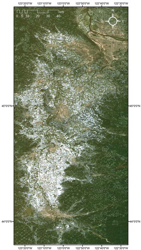
This research was conducted across a 25,303 km² area of the Willamette River basin and nearby drainages in western Oregon and southwestern Washington. The study area was bounded on the east, west, and south by consistently present footprints of Landsat imagery and on the north by the outer extent of the greater Portland metropolitan area. The study area included all traditional crop productions in the Willamette Valley and much of the forests on west slopes of the Cascade and east slopes of the Coastal mountain ranges, along with several large areas of urban development. The overall landscape was dominated by forests covering 67.8% of the area, followed by perennial crops, annually disturbed agriculture, and urban development on 14.4%, 8.1%, and 7.9% of the area, respectively, with the final 1.8% of the area lacking clear consensus among these four groups (Mueller-Warrant, Whittaker, et al. 2015). The Landsat 5 colour composite image of the study area taken on 12 August 2010 was representative of some of the best satellite imagery available to us (Figure 1). It was free of defects that existed in most of the Landsat 7 images and was also essentially cloud-free, a relatively rare occurrence in western Oregon.

Figure 1. Landsat 5 colour composite from 12 August 2010, representative of the best satellite imagery available for the study area, with no clouds needing to be masked out.

3. Methods

3.1. Classification rasters used as input data

In our previous research, remote-sensing classification rasters from the 2004 to the 2011 harvests were developed using ground-truth data from annual drive-by surveys of 3200–7100 fields in combination with a variety of imagery sources, including 30 m Landsat, 250 m Moderate Resolution Imaging Spectroradiometer (MODIS), and 1 m National Agriculture Imagery Program (NAIP), all resampled to common 30 m resolution (Mueller-Warrant et al. 2011; Mueller-Warrant, Whittaker, et al. 2015). In brief, from the list of crop types, stand establishment stages, and crop-management practices observed in the drive-by surveys, 46 crop-management combinations were defined that represented around 99% of the agricultural field area in western Oregon. An additional 11 classes from United States Department of Agriculture (USDA)–National Agriculture Statistics Service (NASS) CDLs (Anonymous 2007) were added to the ground-truth data to represent predominant forest and urban development land uses. Maximum likelihood classifications were conducted for a series of cases consisting of increasing numbers of satellite imagery dates and decreasing total cloud-free extents, merging the results by use of whichever case possessed the highest number of bands at a given location. Following the conclusion of these pixel-based classification methods, we conducted majority-rule reclassification of objects defined by the 2004 CLU fields as subsequently modified in-house based on discovering during our drive-by field surveys that growers had split particular larger fields up into multiple smaller ones. Object-based reclassification was performed using ArcGIS™ Raster Algebra to combine field object numbers with pixel class values in a way that could then be imported into spreadsheets and summarized to identify the most common (majority-rule), second most common, third most common, etc. land-use classes present within each field. When the second-place values were tested in cases where majority-rule classes had been found to be incorrect on the basis of ground-truth training data, the second-place values agreed with the ground-truth training data an average of 60% of the time. Although this procedure provided no indication of where and when to replace majority-rule data with second-place values, these results did imply that such replacements might be useful if other evidence could locate the probable sites and years of misclassification. We also developed 7-year plurality-rule definitions of areas dominated by one of four super-groups of the original 57 categories (Table 1: 19 classes of annually disturbed agriculture, 20 classes of established perennial crops, 13 classes of forests, and five classes of urban development). The final step in this previous research was the development of synthetic ground-truth data for 2004, which allowed us to classify 49 out of the 57 categories present in the succeeding seven years.

Table 1. Land-use descriptions for 19 classes of annually disturbed agriculture, 20 classes of established perennial crops, 13 classes of forests and other natural landscapes, and five classes of urban development, along with counts of permissible year-to-year transitions either from previous or into current land-use classes.

		Counts of allowed transitions between general category groups and each row’s specific class, both from a specific class the previous year into a general class group and from a general class group the previous year into a specific class
		Annually disturbed agriculture		Established perennial crops		Forest and other natural landscapes		Urban development
No.	Class description†	From	Into	From	Into	From	Into	From	Into
19 classes of annually disturbed agriculture
1	Bare ground in fall not any other class	17	18	10	12	0	2	2	2
2	Full straw Italian ryegrass	16	3	3	0	0	0	0	0
3	Spring-plant new grass seed stands	17	18	11	10	0	0	0	0
12	Fall-plant Italian ryegrass	17	18	3	10	0	0	0	0
13	Fall-plant perennial ryegrass	17	15	7	6	0	0	0	0
14	Fall-plant tall fescue	17	15	7	6	0	0	0	0
15	Fall-plant clover	17	18	4	9	0	0	0	0
16	Wheat and oats	17	18	7	12	0	0	0	0
17	Meadowfoam	17	18	4	11	0	0	0	0
27	Corn and sudangrass	17	18	6	12	0	0	0	0
30	Fallow	17	18	10	12	0	2	2	2
35	Beans	17	18	6	12	0	0	0	0
36	Flowers	17	18	5	12	0	0	0	2
40	Other fall-plant/no-till grass seed crops	17	16	9	6	0	0	0	0
41	Spring-plant peas or other unidentified	17	18	12	11	0	0	0	0
42	New planting hops, filberts, blueberries	1	19	3	12	1	1	0	2
43	New planting alfalfa or vetch	17	18	7	9	0	0	0	0
44	Volunteer Italian ryegrass as pasture	16	3	3	0	0	0	0	0
55	Brassicaceae	16	17	6	11	0	0	0	0
Group totals		304	304	123	173	1	5	4	8
20 classes of established perennial agriculture
4	Established perennial ryegrass	15	3	4	1	0	0	0	0
5	Established orchardgrass	14	3	4	1	0	0	0	0
6	Established tall fescue	15	4	4	1	0	0	0	0
7	Pasture	17	18	6	11	0	0	2	2
8	Established clover	15	2	6	1	0	0	0	0
9	Established mint	8	1	1	1	0	0	0	0
10	Haycrop	17	18	6	11	0	0	0	2
18	Established bentgrass	14	2	4	1	0	0	0	0
19	Established fine fescue	14	2	4	1	0	0	0	0
21	Wildrice lagoons	0	2	2	2	0	1	0	0
22	Wetland restoration	0	2	2	2	0	1	0	0
23	Established alfalfa	15	1	3	1	0	0	0	0
24	Established blueberries	0	1	4	1	0	0	0	0
25	Filbert orchard	0	12	3	8	0	0	0	0
26	Caneberry	0	13	3	7	0	0	0	2
28	Nursery crops	12	15	7	8	0	0	2	2
29	Apple, cherry, and other tree fruits	0	13	1	9	0	0	0	2
32	Vineyard	0	3	1	2	0	0	0	0
38	Hop	0	1	1	1	0	0	0	0
56	Strawberry	17	6	6	2	0	0	0	0
Group totals		173	122	72	72	0	2	4	10
13 classes of forests/other natural landscapes
11	Poplars	3	1	0	0	1	1	0	0
20	Christmas tree plantations	2	0	0	0	2	2	0	0
33	Reforestation projects	0	0	0	0	3	1	0	0
34	Assorted other lowland forest	0	0	0	0	1	1	0	0
37	Oaks	0	0	0	0	1	1	0	0
39	Shrubs and wildlife refuges	0	0	0	0	1	1	0	0
45	NLCD 11 open water	0	0	0	0	1	1	0	0
46	NLCD 90 woody wetlands	0	0	0	0	1	1	0	0
47	NLCD 95 herbaceous wetlands	0	0	2	0	1	1	0	0
51	NLCD 41 deciduous forest	0	0	0	0	1	1	0	0
52	NLCD 43 evergreen forest	0	0	0	0	1	3	0	0
53	NLCD 44 mixed forest	0	0	0	0	1	1	0	0
54	NLCD 53 scrub/shrub	0	0	0	0	1	1	0	0
Group totals		5	1	2	0	16	16	0	0
5 classes of urban development
31	Mixed grass and buildings	4	2	5	2	0	0	1	1
48	NLCD 21 developed open space	4	2	5	2	0	0	2	1
49	NLCD 22 developed low intensity	0	0	0	0	0	0	2	2
50	NLCD 23 developed medium intensity	0	0	0	0	0	0	2	2
57	NLCD 24 developed high intensity	0	0	0	0	0	0	1	2
Group totals		8	4	10	4	0	0	8	8
Totals for all 57 classes		490	431	207	249	17	23	16	26

†See Figure 1 for full details of permissible and forbidden year-to-year land-use sequences. The ‘From’ columns list the total number of permitted transitions coming from the 57 specific crops and other land uses listed on the left side of the table and going into each of the four general groups. The ‘Into’ columns list the total number of permitted transitions coming from each of the four general groups and going into the 57 specific crops.

3.2. Definition of permissible and forbidden year-to-year transitions

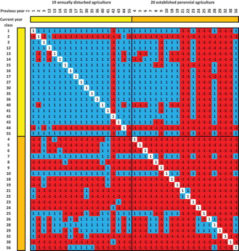
The 57 land-use categories from the previous remote-sensing classifications were used to create a year-to-year transition matrix of rows and columns in a spreadsheet, with the 57 rows corresponding to land-use classification categories for a given year, the 57 columns corresponding to categories in the immediately preceding year, and values of −1 or +1 in the row-by-column intersections indicating whether a specific year-to-year sequence was either forbidden or allowed (Figure 2). Forbidden transitions included those logically inconsistent with definitions of how perennial crops are grown, those banned by public land-use laws, and those extremely unlikely to occur due to inherent economic costs. The allowed transitions were coded in Python scripts as lists with between 1 and 34 entries of the classification categories in the previous year that would be logically consistent with each specific land use in the current year. The rules in this table were primarily constructed using our collective experience advising growers and conducting research with grass seed crops over the past 30 years (Mueller-Warrant, Mellbye, and Aldrich-Markham 1991; Mueller-Warrant 1994; Mueller-Warrant and Rosato 2002a, 2002b, 2005; Steiner et al. 2006; Mueller-Warrant, Whittaker, and Young III 2008; Griffith et al. 2011; Hoag et al. 2012; Mueller-Warrant, Whittaker, et al. 2015). Strict land-use laws and regulations in Oregon governing both forest management and urban development served as the basis for prohibiting most transitions into new urban development or out of forest. Table 1 provides descriptions of each of the 57 land uses, and a summary of the number of permissible transitions among the 57 classes for both directions in time in terms of the four large super-groups (annually disturbed agriculture, established perennial crops, forests, and urban development).

Figure 2. Year-to-year land-use transition matrix showing forbidden sequences (−1) in red and permitted sequences (1) in blue for off-diagonal cases and white for diagonals. Yellow and brown denote 19 cases of annually disturbed agriculture and 20 established perennial crops. Transitions involving 13 forest and five urban development classes have been excluded. Previous-year classes are listed across the top (x-axis) and current-year classes are listed on the left-hand side (y-axis). Class descriptions are provided in Table 1.

3.3. Detection of inconsistent land-use sequences

The original classification rasters for each year from 2004 to 2011 were used to identify inconsistent land-use sequences through the use of the InList() Map Algebra command in ArcGIS™ Spatial Analyst (first action block in flow chart of Figure 3). For each pair of years and each of the 57 categories in the second-year raster, the InList() command was presented with the first-year raster, followed by a series of 34 constant rasters that were valued either as 0 or as each of the up to 34 permitted transition values (Figure 2 and Tables 1 and 2). The IsNull() command was then used to define the area not covered by the InList() output raster, which was intersected by the specific category being tested in the second-year raster. These commands were run in Python scripts calling the ‘arcpy.sa’ module to speed up the process, reduce errors, and maintain a more easily reused archive compared with manually entering them in the ArcGIS™ Raster Calculator interface (scripts are available for download from the ‘Related Topics/Python Scripts’ link at http://www.ars.usda.gov/pandp/people/people.htm?personid=4006). All 57 rasters produced for each pair of years were then merged with a deeply nested series of Con(IsNull()) commands prepared in Excel and pasted into the Raster Calculator interface or created directly in Python. The resulting rasters were labelled as ‘nookXXYYchk??’, with XX from 04 to 10 and YY from 05 to 11 (rasters in lower left-hand corner of flow chart of Figure 3). The rasters identifying positions of illogical year-to-year land-use sequences were multiplied by the 7-year majority-rule-over-time four-group reclassification raster to determine the area of inconsistent land-use sequences within each broad group, with annually disturbed and perennial crop agriculture subsequently merged to simplify the tabular presentation of results (Table 3).

Table 2. Rules for selecting and changing inconsistent classification values during correction-cycle iterations.

Iterations	Selection rules†	Sources of new values
1	Italian ryegrass class 2 must always follow either classes 2, 12, or 44; Italian ryegrass class 12 highly unlikely to follow class 2	Fixed value (class 12); Fixed value (class 2)
2–3	Middle year out of 3 or 5 years inconsistent with other 2 or 4 years; Final year inconsistent after 2, 3, or 4 consecutive allowed transitions; First year inconsistent before 2, 3, or 4 allowed transitions	Second most common value within previous CLU object-based reclassification
4–16	Any inconsistent class over-represented within county-wide area by more than 10%, 5%, 2%, or 0% relative to official crop production summaries in iterations 4–6, 7–9, 10–12, and 13–16, respectively, as long as the potential substitution values themselves were currently under-represented within the county	Second most common value from previous CLU reclassification in iterations 4–5, 7–8, 10–11, 13–14, and 16; Majority-rule value in iterations 6, 9, 12, and 15
17–25	Any inconsistent class over-represented within county-wide area by more than 5% or 0% relative to official crop production summaries in iterations 17–19 and 20–25, respectively, as long as the potential substitution values themselves were not already over-represented within the county	Second most common value from previous CLU reclassification in iterations 17–18, 20–21, 23, and 25; Majority-rule value in iterations 19, 22, and 24
26–44	Any inconsistent class in odd years in even-numbered iterations or even years in odd-numbered iterations over-represented within county-wide area by more than 0% relative to official crop production summaries; Any inconsistent class in even years in even-numbered iterations or odd years in odd-numbered iterations over-represented within county-wide area by more than 0% relative to official crop production summaries	Second most common value from previous CLU reclassification for even/odd or odd/even cases; Majority-rule value for even/even or odd/odd cases
45–128	Random choice within counties and years among any inconsistent class over-represented within county-wide area by more than 0% relative to official crop production summaries: purely random choice for iterations 45–69, Markov chain repeat probabilities of ⅔ and ¾ for iterations 70–119 and 120–128	Second most common value from previous CLU reclassification for random choice = TRUE; Majority-rule value for random choice = FALSE
129–130	Middle year out of 5 years (iteration 129) or 3 years (iteration 130) inconsistent with Italian ryegrass (classes 2, 12, or 44) in the other 4 or 2 years	Fixed value (class 12)

† Flow chart to which these rules apply is provided as Figure 3.

Table 3. Accuracy of original and correction iteration 1 classification rasters from 2004 to 2011, and year-to-year sequence inconsistency rates after correction iteration 1.

Starting year	Overall classification accuracy†		Ending year	Year-to-year land-use sequence inconsistency rates
	Original data	Correction iteration 1		Agriculture	Forest	Urban development	All groups
	(%)			(% of category area participating in logical inconsistencies)
2004	96.5	96.5	2005	34.6	0.67	2.66	9.84
2005	64.9	65.2	2006	23.9	0.61	2.01	6.86
2006	66.8	66.7	2007	24.7	0.61	2.54	7.15
2007	66.0	66.1	2008	17.4	0.47	1.73	5.00
2008	74.2	73.6	2009	16.5	0.62	2.13	4.65
2009	66.4	66.1	2010	34.9	0.72	3.25	9.33
2010	62.2	62.5	2011	32.2	0.75	3.09	8.78
2011	64.1	64.2	– –	– –	– –	– –	– –
Average				26.3	0.64	2.48	7.37

†Classification accuracy for 57 categories is relative to ground-truth training set modified by correcting errors between classes 2 and 12 and removal of all other year-to-year inconsistencies for harvest years identified as starting year. Original and correction iteration 1 refer to classification rasters before and after changes with classes 2 and 12. Land-use sequence inconsistency is from one year to the next, with agriculture combining 19 annually disturbed and 20 established perennial classes, and includes correction of errors between classes 2 and 12.

Figure 3. Flow chart of key steps in the correction-cycle iteration process. Rules for changing the classification values of selected subsets of inconsistencies during each iteration are provided in Table 2.

While there were 2519 possible illogical land-use sequences from one year to the next, the 100 and 400 most common ones accounted for averages of 78% and 97%, respectively, of all inconsistencies (data not shown). Some land-use classes belonged to inconsistencies at similar rates as both starting and ending classes in the year-to-year transitions. Common examples of this behaviour included pasture (class 7), haycrop (class 10), Christmas tree plantations (class 20), filbert orchards (class 25), assorted other lowland forest (class 34), and vineyards (class 32). In contrast, certain other land-use classes often occurred in the ending year of an inconsistent transition while seldom occurring in the starting year. Common examples of this behaviour were established perennial ryegrass (class 4) and established tall fescue (class 6) grown for seed. Finally, some land-use classes often occurred in the starting year of an inconsistent transition while seldom occurring in the ending year. Common examples of this behaviour were full straw Italian ryegrass (class 2) and normal fall-plant Italian ryegrass (class 12). The two most common logically inconsistent transitions for each of the seven pairs of years included the transitions from classes 49 to 48, 48 to 34, 34 to 7 (three times), 7 to 37, 7 to 34 (two times), 12 to 6, 34 to 10, 33 to 7, 20 to 7, 25 to 34, and 34 to 37. These 11 specific cases themselves accounted for a total of 13.8% of all forbidden transitions.

The same procedures for detecting inconsistent land-use sequences in the original classification rasters were also applied to the original ground-truth training data in order to identify and remove any year-to-year inconsistencies without attempting to determine which year’s ground-truth data was in error. The large number of ground-truth data points made the original remote-sensing classifications relatively insensitive to the presence of small numbers of errors in the ground-truth data (Mueller-Warrant, Whittaker, et al. 2015). The large number of ground-truth data points also meant that removing data from both years in cases of inconsistent year-to-year transitions in the ground-truth data would have only a minor impact on the measurements of classification accuracy.

3.4. Selection of individual years as most likely being in error

Multiple approaches exist for selecting which year within a pair of years had most likely been misclassified. The first method we used dealt with two highly similar land-use classes for Italian ryegrass seed production, Italian ryegrass grown using either full straw chop, volunteer stand reseeding (class 2), or normal fall-planting (class 12) methods (Table 2 and Figure 3). Normal fall-planted production of Italian ryegrass grown for seed begins with mid- to late-summer tillage for seedbed preparation, planting of the crop in early fall in rows at seeding rates of 10–15 kg ha⁻¹, fertilization in spring, harvest in early summer, and processing of the straw left behind after combining by baling to remove it or flail chopping to speed its decomposition. The full straw chop volunteer stand reseeding method sometimes used in subsequent years eliminates yearly tillage and relies on the 100 kg ha⁻¹ or more of shattered seed not captured in the combine as the sole, albeit excessive, source of new plants for the next growing season. By definition, full straw chop volunteer stand Italian ryegrass production in one year was dependent on the presence of some version of Italian ryegrass production in the previous year. We used this requirement to change the classification of pixels from class 2 to class 12 in cases where the previous year’s crop was not Italian ryegrass (Table 2 and Figure 3). Because most seed growers who adopt the full straw chop volunteer stand reseeding method tend to continue using it for multiple years, we also changed pixels from class 12 into class 2 in cases where they had been class 2 in the immediately preceding year. These two changes were applied to both ground-truth data and remote-sensing classification results before any other procedures for detecting and correcting year-to-year inconsistencies, and are referred to as the iteration number 1 correction.

One of the simplest ways we used to identify which year within a sequence of years was most likely in error was to combine results from two pairs of years having a common middle year (Tables 2 and 4). An extension to this approach was to test blocks of four year-to-year transitions (derived from five years of original classification rasters) with the restriction that transitions from first to second and from fourth to fifth years were allowed land-use sequences, whereas the forbidden transitions from second to third and from third to fourth years were ones probably including a misclassified third year (Tables 2 and 5).

Table 4. Land-use sequence inconsistency rates after classification correction iteration 1 for agriculture, forest, and urban development for the middle year of 3-year-long periods.

Starting year	Middle year	Ending year	Year-to-year land-use sequence inconsistency rates
			Agriculture		Forest		Urban development
			Once	Twice	Once	Twice	Once	Twice
			(% of category area participating in logical inconsistencies)
2004	2005	2006	31.32	13.59	0.37	0.45	1.87	1.40
2005	2006	2007	21.89	13.36	0.35	0.44	1.59	1.48
2006	2007	2008	26.98	7.56	0.48	0.31	1.82	1.23
2007	2008	2009	22.51	5.69	0.47	0.31	1.44	1.21
2008	2009	2010	32.45	9.47	0.38	0.48	1.82	1.78
2009	2010	2011	20.45	23.31	0.17	0.65	1.05	2.63
Average			25.93	12.16	0.37	0.44	1.60	1.62

Table 5. Land-use sequence inconsistency rates after classification correction iteration 1 for agriculture, forest, urban development, and all groups for the middle year of 5-year-long periods in the absence of any transition errors from first to second and fourth to fifth years.

Starting year	Middle year	Ending year	Year-to-year land-use sequence inconsistency rates
			Agriculture	Forest	Urban development	All groups
			(% of category area participating in logical inconsistencies)
2004	2006	2008	4.23	0.07	0.36	1.09
2005	2007	2009	2.54	0.04	0.15	0.73
2006	2008	2010	1.34	0.03	0.07	0.37
2007	2009	2011	2.35	0.02	0.09	0.59
Average			2.61	0.04	0.17	0.69

A slightly more elaborate procedure was to check for inconsistent transitions after a period of two or more consecutive years of established perennial crops or other difficult-to-change land uses (Table 2 and Figure 3). Classes falling under this category were all of the established perennial crops, forests and other natural landscapes, and urban development. Implementing this test required that the classification categories remain the same for a period of two or more years before the occurrence of an inconsistent year-to-year transition terminating the continuous crop or other repeating land uses. Because some of the annual crops (e.g. Italian ryegrass as class 2 or 12) were grown repeatedly on the same fields, the selection process did not have to exclude annually disturbed crops, although only a few of the transitions among annually disturbed agricultural crops were prohibited.

A similar procedure was to check for inconsistent year-to-year transitions at the start of new stands of an established perennial crop and other continuing land use (Table 2 and Figure 3). Such tests were implemented provided that the new land uses remained in place for periods of two, three, or four consecutive years after the transition whose consistency was being tested. As an example, established perennial ryegrass (class 4) was only allowed to follow either itself or three other classes: spring planting of new grass seed stands (class 3), fall-planted perennial ryegrass (class 13), and spring-planted peas and other unidentified crops (class 41). Any other classifications immediately preceding established perennial ryegrass were viewed as indicating year-to-year inconsistency.

3.5. Correction of classification errors

Correction of classification rasters based on identified year-to-year inconsistencies was conducted in a series of cyclic iterations building on results from each previous iteration (Figure 3). Changed output rasters from each iteration served as input rasters for the next iteration, with recalculation of year-to-year inconsistency. The first corrective iteration comprised swapping classes 2 and 12 in cases where the alternate version of Italian ryegrass production was more consistent with the land-use sequence (details provided in the beginning of Section 3.4).

The second type of correction, employed in iterations 2 and 3, was based on cases in which classifications of the middle year out of three or five years, the beginning year out of three, four, or five years, or the ending year out of three, four, or five years were inconsistent relative to classes in the other years, provided that the overall classification accuracy improved when the CLU second-place classification category was substituted for the original majority-rule category (Table 2 and Figure 3). When more than one change per general selection method (middle, first, or last year inconsistent) per year improved accuracy, we only used whichever one gave the largest improvement, limiting the total possible rules for selecting changes to a maximum of three per year. Iteration 3 repeated the selection tests from iteration 2 but applied them to the revised rasters produced in iteration 2 to determine whether any additional changes would be beneficial.

The third general type of correction, employed in iterations 4–128, used the same methods as in iterations 2 and 3 to identify year-to-year inconsistencies, but with a variety of alternative means for changing values (Table 2 and Figure 3). County-wide estimates of grass seed, legumes, and cereal production area from the Oregon State University (OSU) Extension Service and USDA-NASS (Young III 2006, 2007, 2008, 2009, 2010, 2011, 2012) served as external sources of information to help guide the choice of when to replace given crops with alternatives. This procedure was initially implemented by imposing three selection criteria simultaneously. First, a given year’s pixel had to be detected as being part of a year-to-year sequence inconsistency, although without requiring evidence of which particular year was in error. Second, the existing classification category had to be one that was over-represented within a county for the year. Third, the second-place class from the field-based majority-rule (pixel to object conversion) analysis (under consideration to replace the existing value) had to be one that was under-represented within a county for that year. Crops and land uses other than those representing grass seed, legumes, and cereals were not allowed to change. Because of the possibility that the wrong year’s classification would be changed, this general procedure was repeated in cycles of testing for year-to-year inconsistency, followed by the changing of classification values, until the values stabilized.

After multiple-iteration stability occurred, we switched from using the second-place class back to the majority-rule class of the field objects to check whether that would decrease the year-to-year inconsistency or increase the overall accuracy given the entirety of the changes that had occurred in all previous correction iterations (Table 2 and Figure 3). After classifications stabilized using majority-rule replacement (typically only requiring a single iteration), we reverted to second-place replacement while reducing the requirement for qualifying as over- or under-represented from ±10% down to ±5% discrepancy in area (iterations 7–9). Cycles of switching between second-place and majority-rule replacement continued in concert with further lowering of the over- and under-represented qualification test percentage until classifications were stable and the qualification test levels were next 2% (iterations 10–12) and finally 0% (iterations 13–16).

Once classification rasters stabilized after multiple iterations of testing year-to-year consistency followed by replacement of overabundant classes with under-represented classes in both years, we relaxed the constraints on which classes could change to allow over-represented classes to change into either any under-represented class (as carried out previously) or any class not defined by the external OSU/NASS data (iterations 17–25) (Table 2 and Figure 3). Once this particular method of correction had stabilized, we entirely removed testing for under-representation of the replacement pixel categories, instead adopting an approach of simply alternating second-place and majority-rule values as the replacement choice in consecutive correction iterations. Selection from within these two choices alternated in a fixed pattern of even years receiving majority-rule values and odd years receiving second-place values in one iteration, and vice versa in the next iteration, from iterations 26 to 44. Assignment to either majority-rule or second-place values was carried out on a random basis within counties and years in iterations 45–69, and using Markov chain models with first a two-third chance of staying the same from one iteration to the next (iterations 70–119) and then a three-quarter chance of staying the same (iterations 120–128).

The final means for correcting data, used in iterations 129 and 130, located all cases in which a crop that could be mistaken for Italian ryegrass (class 2, 12, or 44) was present for a single year in between years classified as Italian ryegrass, followed by changing those data to class 12 (Table 2 and Figure 3). Crops viewed as most likely to be confused with Italian ryegrass included perennial ryegrass (class 4 or 13), tall fescue (class 6 or 14), and cereals (class 16). This requirement represented an extension of the year-to-year rules over those previously used, but potentially risked classifying too large of an area as Italian ryegrass. To limit this possibility, we initially (in iteration 129) only made the changes in cases where Italian ryegrass was present for both years before and the two years after the year in question, and then subsequently (in iteration 130) relaxed the requirement down to just single years of Italian ryegrass before and after the year in question.

The order in which these various corrections were applied to the data was primarily based on a desire to minimize that chance that changes made earlier in the correction process would impair the ability of subsequently tested methods to potentially improve year-to-year consistency even further (Table 2 and Figure 3). We performed this by first using methods for which we had the highest confidence that any changes they produced would probably be correct. The changes between classes 2 and 12 made in iteration 1 were by their very definitions almost certain to have no negative effects on the performance of any of the other methods used in the later iterations. The changes made in iterations 2 and 3 to specific years identified as probably being in error based on the land-use sequences of which they were a part were more likely than not the correct changes. Any changes made in iterations 2 and 3 that truly were in error stood a good chance of being flagged as part of the remaining year-to-year inconsistencies during iterations 4–128, and potentially corrected. The various methods used to change the data during iterations 4–128 were introduced in a series of gradually less-restrictive definitions to allow land-use sequences the potential to stabilize before opening up even more of the data to substitution of either second-place or majority-rule values. It is possible that our caution in gradually lowering the thresholds for defining under- and over-abundance relative to countywide agricultural statistics summary data from 10% to 5% to 2% to 0% during iterations 4–25 was unnecessary, but at worst we simply conducted several extra iterations before reaching stability for those methods. The final change (iterations 129 and 130) was the only one made outside of the confines of majority-rule or second-place classes, and was left to the end because it departed from the set of options that we knew had an average 60% chance of being correct whenever the original values were in error. We did not explicitly test the performance of other possible orders for the methods of changing (and potentially correcting) the data. One common feature of all methods used prior to iteration 26 (as well as those of iterations 129 and 130) was that by their very nature they tended to exhaust all possible changes among the eight years of land-use data. Changes made during iterations 26–128, in contrast, could never fully exhaust the possibility of changes as long as alternatives were limited to the majority-rule and second-place class values.

3.6. Accuracy assessment methods

Reference data to support accuracy assessment and validation of the original remote-sensing classifications included a random half of the pixels for fields surveyed in western Oregon agricultural land and the 11 NASS-CDL classes used to represent forests and urban areas. User and producer classification accuracy and the kappa coefficient (κ) were calculated for all contingency (error) matrices using methods described by Congalton (1991) and Mather (2004). Ground-truth training and validation data sets were adjusted by random subsampling on a class-by-class basis to possess nearly identical numbers of pixels (± 0.5%) within all individual classification categories. Variation in size did exist among categories, with the minor land-use categories possessing fewer pixels than the major land-use categories. Maximum pixel counts per class were generally limited to 20,000 each for training and validation data sets. Year-to-year land-use sequence inconsistency rates were calculated using an ArcGIS™ Raster Algebra implementation of the matrix of permissible and forbidden transitions (Figure 1), followed by subdivision of the results into annually disturbed agriculture, perennial crops, forest, and urban development. The two agricultural groups were pooled for summarizing the results because misclassifications often included changes between annual disturbance and perennial crops (Table 3–7).

Table 6. Land-use sequence inconsistency rates after classification correction iteration 1 for agriculture, forest, urban development, and all groups for the final year of 3-, 4-, and 5-year-long periods terminating with final-year transition errors.

Starting year	Duration before transition error	Year of apparent error	Year-to-year land-use sequence inconsistency rates
			Agriculture	Forest	Urban development	All conditions
	(year)		(% of category area participating in logical inconsistencies)
2004	2	2006	1.05	0.08	0.04	1.26
2005	2	2007	1.36	0.04	0.02	1.60
2006	2	2008	1.27	0.09	0.03	1.56
2007	2	2009	1.13	0.06	0.03	1.28
2008	2	2010	2.87	0.08	0.04	3.26
2009	2	2011	0.87	0.04	0.01	1.04
2004	3	2007	0.51	0.01	0.01	0.57
2005	3	2008	0.50	0.01	0.00	0.55
2006	3	2009	0.65	0.01	0.00	0.69
2007	3	2010	1.17	0.00	0.00	1.28
2008	3	2011	0.48	0.00	0.00	0.55
2004	4	2008	0.25	0.00	0.00	0.27
2005	4	2009	0.43	0.00	0.00	0.43
2006	4	2010	0.73	0.00	0.00	0.76
2007	4	2011	0.23	0.00	0.00	0.25

Table 7. Land-use sequence inconsistency rates after classification correction iteration 1 for agriculture, forest, urban development, and all groups for the first year of 3-, 4-, and 5-year-long periods beginning with first-year transition errors.

Starting year	Duration after transition error	Ending year	Year-to-year land-use sequence inconsistency rates
			Agriculture	Forest	Urban development	All conditions
	(year)		(% of category area participating in logical inconsistencies)
2004	2	2006	2.50	0.04	0.02	2.74
2005	2	2007	1.54	0.09	0.03	1.87
2006	2	2008	1.51	0.05	0.04	1.84
2007	2	2009	1.57	0.06	0.02	1.97
2008	2	2010	0.70	0.07	0.01	0.87
2009	2	2011	1.24	0.03	0.04	1.36
2004	3	2007	1.33	0.01	0.01	1.38
2005	3	2008	0.64	0.01	0.00	0.72
2006	3	2009	0.81	0.00	0.00	0.96
2007	3	2010	0.58	0.00	0.00	0.75
2008	3	2011	0.29	0.03	0.00	0.35
2004	4	2008	0.80	0.00	0.00	0.80
2005	4	2009	0.38	0.00	0.00	0.43
2006	4	2010	0.34	0.00	0.00	0.39
2007	4	2011	0.30	0.00	0.00	0.37

4. Results and discussion

4.1. Detection and correction of classification errors involving Italian ryegrass classes

The first correction (iteration 1) applied to both classification and ground-truth data was insistence that full straw volunteer stand reseeding of Italian ryegrass (class 2) could occur only if the previous crop had actually been some type of Italian ryegrass production (classes 2, 12, and 44). We also changed any occurrences of fall-plant Italian ryegrass (class 12) in the first year after full straw volunteer stand reseeding Italian ryegrass into class 2 because growers seldom switch from the volunteer stand reseeding method back to normal seedbed tillage and planting methods. These changes reduced the average year-to-year inconsistency amongst agricultural crops from 26.7% before any corrections to 26.3% afterwards (Figure 2 and Table 3). To provide a better baseline for evaluating the effects of each subsequent classification correction iteration, the ground-truth rasters used in the original maximum likelihood classifications were modified slightly by eliminating data from both years in any cases of year-to-year inconsistency.

4.2. Detection and correction of classification errors using crop rotation patterns

We categorized 730 of 3249 potential year-to-year transitions among 57 land-use classes as being logically permissible, with the remaining 77.5% forbidden (Figure 2 and Table 1). Most of the annually disturbed agriculture classes were allowed to proceed or follow each other. For example, classification category 1 (bare ground in the fall not in any other class) was allowed to proceed 17 of 19 annually disturbed crops, and only prohibited prior to classes 2 and 44 (which required prior crops of Italian ryegrass). It was also allowed as the subsequent year crop in 18 of 19 cases, and only prohibited after class 42 (highly expensive new plantings of hop, filbert, blueberry, and poplar, which are rarely abandoned immediately). Indeed, the only permissible land uses of any type in the year after class 42 were either a repeat of class 42 or successful establishment of hop (class 38), blueberry (class 24), filbert (class 25), or poplar (class 11). For most of the established perennial crops, there was only one permitted transition coming from the group of 20 established perennial crops and going into a specific crop such as class 4 (established perennial ryegrass), the instance of a perennial crop repeating itself. Three members of the annually disturbed agriculture group, classes 3, 12, and 41, were allowed to transition into class 4. Besides continuing on in their existing categories, the only other transitions generally allowed among urban development classes were changes into the next more highly developed category. Annual agriculture classes 1 (bare ground in the fall) and 30 (fallow), however, were allowed to transition both into and out of the two lowest-intensity urban development categories (classes 31 and 48) as representations of activities such as the construction and demolition of houses and livestock facilities on farms. None of the established perennial agricultural crops were allowed to transition directly into any of the forest categories, although annual agriculture classes 1 and 30 were allowed to follow two specific forest categories, poplars (class 11) and Christmas trees (class 20). No transitions in either direction were allowed between forest and urban development categories, reflecting the strong land-use laws currently in place in Oregon.

Applying the restrictions in Figure 2 to eight years of land-use raster data in western Oregon revealed that an average of 26.3% of the year-to-year transitions after among agricultural classes (after iteration 1 correction of apparent confusion between classes 2 and 12) were illogical, in contrast to only 2.5% of the urban development and 0.6% of the forest transitions (Table 3). Combining results from two separate year-to-year transitions with a common middle year identified that middle year as the one most likely in error on average of 12.2% of agricultural land use (Table 4). Similarly, the middle year out of five years was identified as the one most likely in error on average of 2.6% of agricultural land (Table 5). It was also possible to identify the year following logically consistent land-use sequences lasting two, three, or four years as being the one most probably in error (Table 6). The 2010 classification year was the one with the highest frequency of such errors in all three cases. Multi-year sequences in which the preceding year was the one most probably in error identified 2004 more frequently than any other starting year for sequences running two, three, or four years in length after the apparent error (Table 7). In correction iterations 2 and 3, we only changed data to second-place field values for those specific years and selection methods. Doing so increased the classification accuracy, generating 11 general types of substitutions in iteration 2 and eight more in iteration 3 (Figure 4). These corrections reduced year-to-year inconsistency by large amounts in all seven pairs of consecutive years (Figure 5), while also increasing the classification accuracy modestly.

Figure 4. Classification accuracy by correction-cycle iteration. Labelled arrows indicate iteration at which specific strategies for correcting year-to-year inconsistencies were adopted. Iterations 0 and 1 show conditions before and after adjustment of classes 2 and 12 Italian ryegrass.

F = start of two iterations of fixed-rule second-place substitutions

U = start of 13 iterations of substitutions limited to under-represented classes within counties (two second-place followed by one majority-rule substitution at 10%, 5%, 2%, and 0% discrepancy cut-offs)

O = start of nine iterations of only over-represented classes within counties prohibited in substitutions (two second-place followed by one majority-rule substitution at 5% and 0%, then alternating second-place, majority-rule, second-place at 0%)

A = start of 19 iterations of alternating either even or odd years receiving second-place or majority-rule substitution

R = start of 84 iterations of random choice within counties each year of second-place or majority-rule substitution

Figure 5. Agricultural land year-to-year inconsistency by correction-cycle iteration. Labelled arrows are same as described in Figure 4.

4.3. Detection and correction of classification errors using county-wide crop area

The next 13 correction iterations (from 4 to 16) involved the replacement of original majority-rule values with second-place classification categories for fields with inconsistent land uses at the beginning, middle, or ending years of sequences, but only when twin criteria were met of the pixels under consideration for change being over-represented within county and year relative to the OSU/NASS estimates and the replacement pixels being under-represented (Table 2 and Figure 3). This approach reduced year-to-year land-use inconsistency by iteration 16 to an average of 20.1% of the agricultural area (Figure 5), while either improving overall classification accuracy or leaving it unchanged (Figure 4). More pixels were identified for correction in the first use of this method (iteration 4) than in all 12 subsequent iterations combined. The second application of the same selection criteria and replacement procedures (correction iteration 5) only changed an average of 1534 pixels per year, with very little effect on accuracy and year-to-year inconsistency. In an attempt to disrupt this stability, we next changed pixels back to their original majority-rule values in cases where categories were over-represented by at least 10% within counties and the replacement values were under-represented. While this procedure (iteration 6) changed the values of an average of 6198 pixels, there was very little net effect on either accuracy or year-to-year inconsistency. The next two correction iterations lowered the cut-off for detecting over- or under-representation to 5% discrepancy with OSU/NASS production estimates while resuming use of second-place values in the replacement process. Iteration 7 changed the values of an average of 6811 pixels per year while iteration 8 only changed values of 495 pixels per year. There was very little net effect from either change on accuracy or year-to-year inconsistency (Figures 4 and 5). Reverting to substitution of majority-rule values in iteration 9 only changed an average of 654 pixels per year, with almost no impact on accuracy or year-to-year inconsistency. Lowering the discrepancy level for over- and under-representation in iterations 10 and 11 to 2% only changed the averages of 2788 and 1215 pixels per year, with little net effect on accuracy or year-to-year inconsistency.

Our methods had no difficulty detecting over-represented classes participating in year-to-year inconsistency, as there were 8-year averages of 129,130; 10,678; 168,547; 148,846; 4784; 171,248; and 166,031 such pixels, respectively, in iterations 5–11 (calculated from data underlying Figure 5). The problem was that the second-place values were typically not themselves members of under-represented classes within a county, and therefore failed to meet our selection criteria. Once we had exhausted all options for most safely correcting pixels (iteration 16), we removed the requirement that the second-place values had to be members of under-represented classes, instead only requiring that they not be known members of currently over-represented classes (Table 2 and Figure 3). This change selected larger fractions of the pixels for possible substitution in iterations 17–25, and generated wider swings from one correction iteration to the next regarding which classes were viewed as over-represented and available for change when participating in year-to-year inconsistency. The series of corrections starting at iteration 17 replaced the majority-rule values with the second-place field classification categories for any years in which the existing categories were over-represented and the replacement categories were under-represented. Because these changes were potentially applied to either or both years participating in an inconsistent transition, multiple cycles of this correction were conducted until results stabilized. In the first such iteration, year-to-year inconsistency for agricultural land dropped by an average of 0.2%, with most of the improvement occurring in pairs of years with higher than average year-to-year inconsistency (Figure 5). Alternating the choice of second-place and majority-rule values for the substitution value from iteration to iteration allowed the year-to-year inconsistencies to dissipate partially, although the largest corrections occurred in the first few iterations of this phase. Minor drops in accuracy occurred in iteration 17, likely representing another instance of apparent errors in ground-truth data for a few fields, errors not seen until particular year-to-year inconsistencies were removed. Unlike the situation in iteration 1 for which we did find and remove ground-truth data conflicting with the corrections between classes 2 and 12, we did not identify and correct whichever fields contained ground-truth conflicting with the newly corrected data in iteration 17, because doing so would have opened the project up to the creation of an ever-expanding group of slightly different versions of ground-truth data in successive correction iterations.

4.4. Correction of classification errors using random switching between second-place and majority-rule substitutions

At iteration 26 we abandoned the previous requirement of always using either second-place or majority-rule values as the ones being substituted in any iteration, and instead began alternating use of majority-rule substitutions in even years on even-numbered rounds and in odd years on odd-numbered rounds, and second-place substitutions otherwise. This method generated the largest changes in year-to-year inconsistency seen since those occurring in iteration 2. Changes were the most dramatic for inconsistencies involving either the first or the last year of our classification period (2004 and 2011) when paired with the only years adjacent to them (2005 and 2010), resulting in an 8% reduction in agricultural land-use inconsistency for 2004–2005 and a 4% reduction for 2010–2011 (Figure 5). In effect, what our technique from iterations 26–44 was doing was exploring the possibility that correcting year-to-year inconsistencies required keeping a majority-rule value in some years and substituting the second-place value in the year immediately before or after it, or vice versa. The beginning and ending years of our classification period were more likely to have such changes become fixed in part because they were only subject to selection pressure from one direction in time, unlike the middle six years that could potentially alternate between agreeing with land use in the years either before or after them. After the initial burst of progress when this method was adopted, obvious multiple-iteration pattern repetition (‘zigzags’) developed for all but the first pair of years, with little further progress in reducing year-to-year inconsistency after iteration 28. This pattern suggested the need for longer runs of a given substitution (second-place or majority-rule) before switching to the alternative to allow bridging over periods longer than just a single misclassified year. Unfortunately, many multi-year substitution patterns exist that could potentially bridge gaps between consistent land-use sequences, and we saw little reason to favour any one particular arrangement over another. We therefore decided to assign second-place or majority-rule substitutions on a strictly random basis for pixels meeting the twin requirements of membership in year-to-year inconsistency and over-representation within a county. The first 25 randomly assigned substitutions had equal probability of either substitution occurring, whereas the next 50 were treated as a Markov chain model with a two-third chance of continuing with the same substitution used in the previous round and a one-third chance of switching to the other substitution. The final nine rounds were Markov chains with a three-quarter chance of continuing with the same substitution. The primary limitation on running this search algorithm was that each iteration took approximately 3 hours to complete on a high-end GIS workstation. Long-term progress in the random substitution phase was most clearly seen in the number of pixels changed and potentially corrected in each iteration, which declined from a total of 424,278 pixels in iteration 45 to 345,974 in iteration 128, an 18.5% drop (Figure 6).

Figure 6. Total year-to-year inconsistencies and attempted corrections for all groups by correction-cycle iteration. Labelled arrows are same as described in Figure 4.

After classifications had essentially stabilized by iteration 128, we converted the remaining single-year cases of perennial ryegrass, tall fescue, or cereals into class 12 Italian ryegrass whenever they were surrounded by either one or two consecutive years of Italian ryegrass in the periods both before and after the year in question. The stricter (2-year) requirement converted a total of 70,290 pixels into Italian ryegrass in the period from 2005 to 2010, whereas the looser (1-year) requirement added another 42,376 pixels beyond those of the stricter requirement. Both of these reclassification methods produced similar reductions in year-to-year inconsistency (0.17% and 0.21% lower than conditions after iteration 128 for stricter and looser requirements, respectively). Classification accuracy dropped slightly in most years, although it did increase for the stricter method in 2008 and 2010. Corrected rasters from iteration 130 were then used to measure the apparent duration of land-use continuity for periods beginning in 2004.

4.5. Stand duration

Apparent stand durations given in Tables 8 and 9 (before and after 130 iterations of correcting year-to-year inconsistencies) were distorted by the finite (8-year) length of our classification data, which had the effect of prematurely truncating many new stands (continuous presence of the same land-use class), especially for those with a starting year late in the overall 2004–2011 period. Benefits of correcting year-to-year inconsistencies were most clearly seen in long-lived crops such as orchardgrass, tall fescue, and fine fescue, where average stand ages increased by 0.61, 0.25, and 0.39 years, respectively, with most of the increases due to greater percentages of these crops in the 5+ year age category. Further adjustments that need to be made to the stand age data before it can be used to direct us to the location of shorter or longer than average duration crops will include the detection of normal transition classes before and after the period of continuously established stands. Data available for these purposes include the presence of permitted land-use classes in the year prior to start of the established stand sequences and logical termination classes in the year after the end of the sequences. The termination signal will, of course, be absent for stands that are continuing beyond 2011.

Table 8. Stand ages for major crops and other selected land uses prior to any correction of year-to-year inconsistencies.

Class no.	Crop/land use	Average stand age†	Stand age distribution
			1 year	2 years	3 years	4 years	5+ years
		(years)	(stand age as proportion of the class in %)
4	Established perennial ryegrass	1.96	49.6	27.2	11.9	5.5	5.9
5	Established orchardgrass	2.10	58.6	15.2	8.7	5.8	11.7
6	Established tall fescue	2.23	40.2	26.6	15.8	9.5	7.9
7	Pasture	2.19	42.2	27.7	13.7	8.2	8.3
8	Established clover	1.26	79.3	16.6	3.2	0.9	0.0
12	Italian ryegrass (composite all classes)	3.61	21.3	19.0	14.3	12.1	33.2
16	Wheat and other cereals	1.51	65.2	24.7	6.6	2.0	1.5
19	Established fine fescue	2.32	47.6	18.9	12.4	8.5	12.5
20	Christmas tree plantations	4.81	4.0	14.6	13.8	13.6	54.1
48	NLCD 21 developed open space	4.06	17.6	18.4	10.8	10.7	42.6
49	NLCD 22 developed low intensity	4.59	9.5	13.6	13.0	12.8	51.1
50	NLCD 23 developed medium intensity	5.00	0.0	14.3	14.3	14.3	57.1
57	NLCD 24 developed high intensity	4.88	2.7	14.2	13.9	13.9	55.4
51	NLCD 41 deciduous forest	4.99	0.1	14.3	14.3	14.3	57.0
52	NLCD 43 evergreen forest	5.00	0.0	14.3	14.3	14.3	57.1
53	NLCD 44 mixed forest	5.00	0.0	14.3	14.3	14.3	57.1

†Average stand age was limited to a maximum of 5 years by the length of the classification record starting with each individual year and eliminating (1-year) data for sequences starting in 2011.

Table 9. Stand ages for major crops and other selected land uses after correction iteration 130.

Class no.	Crop/land use	Average stand age	Stand age distribution
			1 year	2 years	3 years	4 years	5+ years
		(years)	(stand age as proportion of the class in %)
4	Established perennial ryegrass	2.15	43.8	27.7	13.6	6.8	8.1
5	Established orchardgrass	2.71	42.1	17.3	11.5	9.0	20.0
6	Established tall fescue	2.48	34.1	25.5	17.5	11.3	11.5
7	Pasture	2.30	40.9	26.8	13.5	8.5	10.3
8	Established clover	1.30	77.1	17.1	4.1	1.5	0.1
12	Italian ryegrass (composite all classes)	3.75	18.5	18.8	14.9	12.5	35.3
16	Wheat and other cereals	1.53	64.5	25.0	6.9	2.0	1.5
19	Established fine fescue	2.71	41.0	16.9	12.7	10.0	19.4
20	Christmas tree plantations	4.81	3.6	14.6	13.9	13.7	54.2
48	NLCD 21 developed open space	4.05	17.4	19.0	10.7	10.6	42.3
49	NLCD 22 developed low intensity	4.59	8.9	14.1	13.2	12.8	51.0
50	NLCD 23 developed medium intensity	5.00	0.0	14.3	14.3	14.3	57.1
57	NLCD 24 developed high intensity	4.89	2.6	14.2	13.9	13.9	55.5
51	NLCD 41 deciduous forest	4.99	0.1	14.3	14.3	14.3	57.0
52	NLCD 43 evergreen forest	5.00	0.0	14.3	14.3	14.3	57.1
53	NLCD 44 mixed forest	5.00	0.1	14.3	14.3	14.3	57.1

The maximum average stand age measurable with the methods used to create Table 9 is 5.0 years, a value shared by classes 50, 51, 52, and 53 (medium-intensity urban development, deciduous forest, evergreen forest, and mixed forest, respectively). The longest duration crop was Italian ryegrass (with classes 2, 12, and 44 grouped together as a single category), with an average continuous re-cropping period of 3.75 years. Over 35% of all Italian ryegrass fields were five or more years in duration. The shortest lived established perennial grass crop was class 4, perennial ryegrass, with an average re-cropping period of 2.15 years. Perennial ryegrass is well-known for dying out by the third year of production.

4.6. Verifying the validity of results from the iterative classification correction process

Once we had completed using the iterative process of identifying year-to-year inconsistencies and attempting to change the classification values of those particular pixels into ones that generated more logically consistent crop rotations, we doubled-checked on whether our techniques had perhaps only succeeded due to unknown factors within the specific ground-truth training data used to create the initial remote-sensing classification rasters in our previous research. We did so primarily by measuring the rates of classification errors and κ against both training and validation data sets at two points near the beginning and two points near the end of the correction process, iterations 0, 1, 128, and 130 (Table 10). If any pattern exists at all across these 130 iterations of correction attempts, it would be that the ground-truth validation data sets seemed to measure slightly higher classification accuracies than the ground-truth training sets. Validation data outperformed training data by averages of 1.02%, 0.74%, 0.75%, and 0.77% accuracy in iterations 0, 1, 128, and 130, respectively (data not presented). Similar differences were present for κ, with validation data outperforming training set data by values of 0.011, 0.008, 0.008, and 0.009, respectively, for the same four iterations (Table 10). Lacking any theoretical perspective for criticizing better accuracy in validation than in training set data, we are left with the conclusion that none of our procedures for correcting the data succeeded simply due to quirks in our random choices for ground-truth training data.

Table 10. Overall classification κ for ground-truth training and validation data sets at correction iterations 0, 1, 128, and 130.

	Iteration 0 κ		Iteration 1 κ		Iteration 128 κ		Iteration 130 κ
Crop year†	Training set	Validation set	Training set	Validation set	Training set	Validation set	Training set	Validation set
2004	0.963	0.963	0.963	0.963	0.963	0.964	0.963	0.964
2005	0.631	0.642	0.633	0.640	0.620	0.627	0.619	0.626
2006	0.651	0.676	0.650	0.672	0.642	0.664	0.642	0.664
2007	0.646	0.671	0.647	0.666	0.643	0.662	0.642	0.662
2008	0.722	0.736	0.715	0.727	0.707	0.720	0.703	0.716
2009	0.651	0.654	0.648	0.650	0.646	0.649	0.645	0.648
2010	0.606	0.609	0.608	0.608	0.612	0.612	0.612	0.611
2011	0.627	0.631	0.628	0.628	0.618	0.618	0.618	0.618
Mean	0.687	0.698	0.686	0.694	0.681	0.689	0.680	0.689

†Classification κ for ground-truth training and validation data for all iterations include removal of both years’ data for any instance of year-to-year inconsistency present at iteration 1.

One final point of interest is how often our attempted corrections truly succeeded in changing the value of the pixels identified for correction. Comparing rasters from iterations 0 and 130, there were totals of 1,201,169; 895,185; 746,868; 910,057; 613,422; 917,858; 1,637,127; and 623,554 pixels ultimately changed in the process of correcting the 2004, 2005, 2006, 2007, 2008, 2009, 2010, and 2011 classification rasters, respectively. Although these were large numbers (totalling 7,545,240 pixels over all eight years), they were dwarfed by the total attempted changes of 40,296,565 pixels over the full 130 iterations (Figure 6). Only 1 out of every 5.34 attempted changes actually stuck, indicating that individual pixels often already possessed the (new) value we were attempting to give them or that their values just kept switching back and forth between the only two options under consideration, the majority-rule value or the second-place alternative from the pixel-based to object-based conversion.

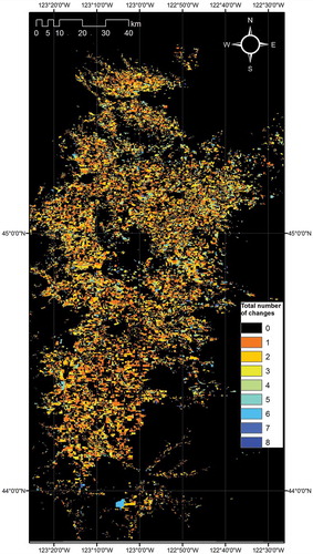
A map of the distribution of changes in pixel classification values (excluding all changes occurring simply among the three highly similar Italian ryegrass categories, classes 2, 12, and 44) between the start and end of the 130 iterations closely matched the location of annual and perennial agriculture, with very few changes occurring in urban development and forested areas (Figure 7). Classifications in nearly 87.8% of the entire area were unchanged in any of the eight years. Changes occurred one, two, three, four, five, six, seven, or eight times over the 8-year-period in 4.9%, 3.3%, 2.0%, 1.1%, 0.6%, 0.2%, 0.06%, or 0.001% of the area, respectively. Within the four superclass land-use categories, 99.7% and 99.1% of pixels in forested and urban development areas, respectively, were unchanged by the 130 iterations, whereas only 57.8% and 40.6% of annually disturbed and perennial crop agriculture pixels, respectively, remained unchanged. It is not surprising that the largest number of the changes during the 130 iterations occurred within the perennial agriculture superclass area, because that group of crops had the most complex set of rules defining allowed and forbidden transitions. Because the original segmentation of our rasters into four superclasses had simply been based on which type of the four super-land uses occurred most often over the period from 2005 to 2011, both annually disturbed and perennial crop agricultural classes frequently coexisted over time at the same locations. Combining both types of agriculture, 46.8% of pixels were unchanged throughout the entire 8-year period, with changes occurring in 21.7%, 14.4%, 8.8%, 4.8%, 2.3%, 1.0%, 0.27%, and 0.005% of the area during totals of one, two, three, four, five, six, seven, and eight times, respectively.

Figure 7. Total number of changes by iteration 130 over the entire eight years. Out of 28,114,889 total pixels, 87.8%, 4.89%, 3.27%, 2.04%, 1.14%, 0.57%, 0.24%, 0.06%, and 0.001% were changed in 0, 1, 2, 3, 4, 5, 6, 7, and 8 of the years, respectively. Changes occurring solely among the three Italian ryegrass classes (2, 12, and 44) have been excluded.

5. Conclusions

Our technique of using a matrix of forbidden and permissible year-to-year land-use (sequence) transitions was quite successful in identifying inconsistencies within our eight years of remote-sensing classifications. How well such procedures would work in other areas with differing mixes of annual and perennial crops, forest, and urban development is uncertain, although the primary issue would clearly be the analyst’s ability to define large fractions of the potential year-to-year sequences as being forbidden. If nearly all transitions were allowed, then the identification of inconsistences would probably be too infrequent to be useful.

The ability to define some particular year as being the one most likely in error in the case of multiple, overlapping year-to-year inconsistencies was critically important in correcting data. Although we focused on the use of second-place classification values remaining from our previous conversion from pixel-based to object-based classifications, there is every reason to believe that other sources of alternate classification values might also be useful. Possible sources could include: (1) lower-order categories (third-place, fourth-place, etc.) from pixel- to object-based conversions; (2) first, second, and third most frequently confused categories from the yearly classification accuracy matrices; (3) other (independent) classification data, including multi-year rasters summarized by majority-rule over time procedures; and (4) countywide reports of agricultural production data although such information is usually not spatially defined at any finer scale than the political subdivision boundaries.

Our second most successful method of correcting year-to-year inconsistencies involved alternating substitutions of second-place and majority-rule values at both ends of identified year-to-year inconsistencies, with one year getting the second-place value whereas the other matching (earlier or later) year got the majority-rule value, followed by switching of those conditions back and forth in the subsequent iterations until corrections stabilized. In order for this procedure to succeed, it was necessary to retest the set of classification data for year-to-year inconsistencies after each iteration of changing pixel values. Pixels that disappeared from the year-to-year inconsistency rasters in subsequent iterations would generally represent cases where consistent land-use sequences before and after the years in question bridged together, thanks to changes made to the questionable year or years in between them. After the dramatic improvements that occurred in the period from iterations 26 to 28 when the use of alternating substitutions was first introduced, the remaining iterations simply provided a gradual drift towards eventual stability. Minor changes to the pattern used to swap between majority-rule and second-place substitutions (a switch first to random selection of which years got which type of substitution followed by Markov chain models) freed the rasters from several bouts of pseudo-stability before the true end of the correction process. The ability of Python and ArcGIS™ to pass data back and forth and run in a semi-automated fashion allowed us to carry this iterative correction process on to its ultimate conclusion.

The corrected rasters represented a clear improvement over the starting versions in terms of their ability to define apparent stand ages for crops of interest. Although further improvement in reducing inconsistencies beyond what was achieved here would be desirable, it was encouraging to see that most of the reductions in year-to-year inconsistency came at relatively little reduction in overall classification accuracy and with no evidence of bias between training and validation data. We are confident the corrected rasters will lead to an improved description of crop rotation patterns in western Oregon agriculture. Our data also verify the general stability of the two other major land uses in the region, namely urban development and forestry.

Acknowledgements

Contribution of USDA-ARS, which provided primary funding for this research. The use of trade, firm, or corporation names in this publication (or page) is for the information and convenience of the reader. Such use does not constitute an official endorsement or approval by the United States Department of Agriculture or the Agricultural Research Service of any product or service to the exclusion of others that may be suitable.

Disclosure statement

No potential conflict of interest was reported by the authors.

Additional information

Funding

Contribution of USDA-ARS provided primary funding for this research.

References

- Anonymous. 2007. USDA, National Agricultural Statistics Service, 2007 Oregon Cropland Data Layer. Accessed 22 January 2015. http://www.nass.usda.gov/research/Cropland/metadata/metadata_or07.htm
- Anonymous. 2009. USDA, Natural Resources Conservation Service, Conservation Effects Assessment Project (CEAP). Accessed 22 January 2015. http://www.nrcs.usda.gov/wps/portal/nrcs/main/national/technical/nra/ceap/
- Congalton, R. G. 1991. “A Review of Assessing the Accuracy of Classifications of Remotely Sensed Data.” Remote Sensing of Environment 37: 35–46. doi:10.1016/0034-4257(91)90048-B.
- Fernandez-Prieto, D. 2002. “An Iterative Approach to Partially Supervised Classification Problems.” International Journal of Remote Sensing 23: 3887–3892. doi:10.1080/01431160210133563.
- Griffith, S. M., G. M. Banowetz, R. P. Dick, G. W. Mueller-Warrant, and G. W. Whittaker. 2011. “Western Oregon Grass Seed Crop Rotation and Straw Residue Effects on Soil Quality.” Agronomy Journal 103: 1124–1131. doi:10.2134/agronj2010.0504.
- Hoag, D. L. K., G. R. Giannico, J. Li, T. Garcia, W. Gerth, M. Mellbye, G. Mueller-Warrant, et al. 2012. “Calapooia Watershed, Oregon: National Institute of Food and Agriculture-Conservation Effects Assessment Project.” Chapter 19. In How to Build Better Agricultural Conservation Programs to Protect Water Quality: The National Institute of Food and Agriculture–Conservation Effects Assessment Project Experience, edited by D. L. Osmond, D. W. Meals, L. K. H. Dana, and M. Arabi, 387. Ankeny, IA: Soil and Water Conservation Society. Hardcover ISBN 978-0-9769432-9-7. Accessed 6 November 2015. http://www.swcs.org/en/publications/building_better_agricultural_conservation_programs/
- Homer, C., C. Huang, L. Yang, B. Wylie, and M. Coan. 2004. “Development of a 2001 National Land Cover Database for the United States.” Photogrammetric Engineering & Remote Sensing 70 (7): 829–840. doi:10.14358/PERS.70.7.829.
- Jiang, H., J. R. Strittholt, P. A. Frost, and N. C. Slosser. 2004. “The Classification of Late Seral Forests in the Pacific Northwest USA Using Landsat ETM+ Imagery.” Remote Sensing of Environment 91: 320–331. doi:10.1016/j.rse.2004.03.016.
- Liu, X.-H., A. K. Skidmore, and H. Van Oosten. 2002. “Integration of Classification Methods for Improvement of Land-Cover Map Accuracy.” ISPRS Journal of Photogrammetry and Remote Sensing 56: 257–268. doi:10.1016/S0924-2716(02)00061-8.
- Lu, D., P. Mausel, E. Brondízio, and E. Moran. 2004. “Change Detection Techniques.” International Journal of Remote Sensing 25: 2365–2401. doi:10.1080/0143116031000139863.
- Lu, D., and Q. Weng. 2007. “A Survey of Image Classification Methods and Techniques for Improving Classification Performance.” International Journal of Remote Sensing 28: 823–870. doi:10.1080/01431160600746456.
- Malpica, J. A., and M. C. Alonso. 2008. “A Method for Change Detection with Multi-Temporal Satellite Images Using the RX Algorithm.” International Archives Photogrammetry, Remote Sensing and Spatial Information Sciences XXXVII (B7): 1631–1636.
- Manandhar, R., I. O. A. Odeh, and T. Ancev. 2009. “Improving the Accuracy of Land Use and Land Cover Classification of Landsat Data Using Post-Classification Enhancement.” Remote Sensing 1: 330–344. doi:10.3390/rs1030330.
- Mather, P. M. 2004. Computer Processing of Remotely-Sensed Images, An Introduction. Third Addition. Chichester, England: John Wiley & Sons.
- Millward, A. A., J. M. Piwowar, and P. J. Howarth. 2006. “Time-Series Analysis of Medium-Resolution, Multisensor Satellite Data for Identifying Landscape Change.” Photogrammetric Engineering & Remote Sensing 72 (6): 653–663. doi:10.14358/PERS.72.6.653.
- Mueller-Warrant, G. W. 1994. “Weed Control in U.S. Grass Seed Crops.” International Herbage Seed Production Research Group Newsletter 21 (Dec): 7–10.
- Mueller-Warrant, G. W., S. M. Griffith, G. M. Banowetz, G. W. Whittaker, and K. M. Trippe. 2015. “Inferring Crop Stand Age and Landuse Duration in the Willamette Valley from Remotely Sensed Data.” In 2013 Seed Production Research, edited by N. Anderson, A. Hulting, D. Walenta, and M. Flowers, 49–53. Corvallis, OR: Oregon State Univ. Extension and USDA-ARS, Ext/CrS 150. Accessed 12 May 2015. http://cropandsoil.oregonstate.edu/content/2013-seed-production-research-report)
- Mueller-Warrant, G. W., S. M. Griffith, G. W. Whittaker, G. M. Banowetz, W. F. Pfender, T. S. Garcia, and G. Giannico. 2012. “Impact of Landuse Patterns and Agricultural Practices on Water Quality in the Calapooia River Basin of Western Oregon.” Journal of Soil and Water Conservation 67 (3): 183–201. doi:10.2489/jswc.67.3.183.
- Mueller-Warrant, G. W., M. E. Mellbye, and S. Aldrich-Markham. 1991. “Pronamide Improves Weed Control in New Grass Plantings Protected by Activated Charcoal.” Journal Applied Seed Products 9: 16–26.
- Mueller-Warrant, G. W., and S. C. Rosato. 2002a. “Weed Control for Stand Duration Perennial Ryegrass Seed Production: I Residue Removed.” Agronomy Journal 94: 1181–1191. doi:10.2134/agronj2002.1181.
- Mueller-Warrant, G. W., and S. C. Rosato. 2002b. “Weed Control for Stand Duration Perennial Ryegrass Seed Production: II Residue Retained.” Agronomy Journal 94: 1192–1203. doi:10.2134/agronj2002.1192.
- Mueller-Warrant, G. W., and S. C. Rosato. 2005. “Weed Control for Tall Fescue Seed Production and Stand Duration without Burning.” Crop Science 45: 2614–2628. doi:10.2135/cropsci2003.0375.
- Mueller-Warrant, G. W., G. W. Whittaker, G. M. Banowetz, S. M. Griffith, and B. L. Barnhart. 2015. “Methods for Improving Accuracy and Extending Results beyond Periods Covered by Traditional Ground-Truth in Remote Sensing Classification of a Complex Landscape.” International Journal of Applied Earth Observation and Geoinformation 38: 115–128. doi:10.1016/j.jag.2015.01.001.
- Mueller-Warrant, G. W., G. W. Whittaker, S. M. Griffith, G. M. Banowetz, B. D. Dugger, T. S. Garcia, G. Giannico, K. L. Boyer, and B. C. McComb. 2011. “Remote Sensing Classification of Grass Seed Cropping Practices in Western Oregon.” International Journal of Remote Sensing 32 (9): 2451–2480. doi:10.1080/01431161003698351.
- Mueller-Warrant, G. W., G. W. Whittaker, and W. C. Young III. 2008. “GIS Analysis of Spatial Clustering and Temporal Change in Weeds of Grass Seed Crops.” Weed Science 56: 647–669. doi:10.1614/WS-07-032.1.
- Nelson, D. 2005. High Yield Grass Seed Production and Water Quality Protection Handbook. Accessed 13 January 2009. http://forages.oregonstate.edu/organizations/seed/osc/brochures/water-quality/index.html
- Nelson, M. A., S. M. Griffith, and J. J. Steiner. 2006. “Tillage Effects on Nitrogen Dynamics and Grass Seed Crop Production in Western Oregon, USA.” Soil Science Society of America Journal 70 (3): 825–831. doi:10.2136/sssaj2005.0248.
- Patekar, P. R., and R. R. Patil. 2014. “Land Use-Land Cover Change Detection Using Remote Sensing and GIS Techniques; Solapur District of Maharashtra, India.” International Journal of Advance Remote Sensing and GIS 3 (1): 499–505.
- Patekar, P. R., and P. L. Unhale. 2013. “Remote Sensing and GIS Application in Change Detection Study Using Multi Temporal Satellite.” International Journal of Advance Remote Sensing and GIS 2 (1): 374–378.
- Rutchey, K., and L. Velcheck. 1994. “Development of an Everglades Vegetation Map Using a SPOT Image the Global Positioning System.” Photogrammetric Engineering and Remote Sensing 60: 767–775.
- Sahajpal, R., X. Zhang, R. C. Izaurralde, I. Gelfand, and G. C. Hurtt. 2014. “Identifying Representative Crop Rotation Patterns and Grassland Loss in the US Western Corn Belt.” Computers and Electronics in Agriculture 108: 173–182. doi:10.1016/j.compag.2014.08.005.
- San Miguel-Ayanz, J., and G. S. Biging. 1996. “An Iterative Classification Approach for Mapping Natural Resources from Satellite Imagery.” International Journal of Remote Sensing 17: 957–981. doi:10.1080/01431169608949058.
- San Miguel-Ayanz, J., and G. S. Biging. 1997. “Comparison of Single-Stage and Multi-Stage Classification Approaches for Cover Type Mapping with TM and SPOT Data.” Remote Sensing of Environment 59: 92–104. doi:10.1016/S0034-4257(96)00109-5.
- Steiner, J. J., G. R. Giannico, S. M. Griffith, M. E. Mellbye, J. L. Li, K. S. Boyer, S. H. Schoenholtz, G. W. Whittaker, G. W. Mueller-Warrant, and G. M. Banowetz. 2004. “Grass Seed Fields, Seasonal Winter Drainages, and Native Fish Habitat in the South Willamette Valley.” In 2003 Seed Production Research, edited by W. C. Young III, 55–56. Corvallis, OR: Oregon State Univ. Extension and USDA-ARS, Ext/CrS 123.
- Steiner, J. J., S. M. Griffith, G. W. Mueller-Warrant, G. W. Whittaker, G. M. Banowetz, and L. F. Elliott. 2006. “Conservation Practices in Western Oregon Perennial Grass Seed Systems. I: Impacts of Direct Seeding and Maximal Residue Management on Production.” Agronomy Journal 98: 177–186. doi:10.2134/agronj2005.0003.
- Stern, A. J., P. C. Doraiswamy, and E. R. Hunt Jr. 2012. “Changes in Crop Rotation in Iowa Determined from the Unites States Department of Agriculture, National Agricultural Statistics Service Cropland Data Layer Product.” Journal of Applied Remote Sensing 3 (1): 1–16.
- Wentz, D. A., B. A. Bonn, K. D. Carpenter, S. R. Hinkle, M. L. Janet, F. S. Rinella, M. A. Uhrich, I. R. Waite, A. Laenen, and K. E. Bencala. 1998. “Water Quality in the Willamette Basin, Oregon, 1991-95.” In U.S. Geological Survey Circular 1161. Washington, DC: U.S. Geological Survey, U.S. Department of the Interior. ISBN 0607892315 (pbk.). https://pubs.er.usgs.gov/publication/cir1161
- Whittaker, G., R. Confesor, S. M. Griffith, R. Färe, S. Grosskopf, J. J. Steiner, G. W. Mueller-Warrant, and G. M. Banowetz. 2009. “A Hybrid Genetic Algorithm for Multiobjective Problems with Activity Analysis-Based Local Search.” European Journal of Operational Research 193: 195–203. doi:10.1016/j.ejor.2007.10.050.
- Whittaker, G. W., R. Confesor, M. D. DiLuzio, and J. G. Arnold. 2010. “Detection of Overparameterization and Overfitting in an Automatic Calibration of SWAT.” Transactions of the ASABE 53: 1487–1499. doi:10.13031/2013.34909.
- Xiuwan, C. 2002. “Using Remote Sensing and GIS to Analyse Land Cover Change and Its Impacts on Regional Sustainable Development.” International Journal of Remote Sensing 23 (1): 107–124. doi:10.1080/01431160010007051.
- Yang, X. 2002. “Satellite Monitoring of Urban Spatial Growth in the Atlanta Metropolitan Area.” Photogrammetric Engineering and Remote Sensing 68 (7): 725–734.
- Young III, W. C. 2006. Extension Estimates for Oregon Forage and Turf Grass Seed Crop Acreage, 2005. Accessed 17 March 2015. http://cropandsoil.oregonstate.edu/system/files/u1473/05ftprod.pdf
- Young III, W. C. 2007. Extension Estimates for Oregon Forage and Turf Grass Seed Crop Acreage, 2006. Accessed 17 March 2015. http://cropandsoil.oregonstate.edu/system/files/u1473/06ftprod.pdf
- Young III, W. C. 2008. Extension Estimates for Oregon Forage and Turf Grass Seed Crop Acreage, 2007. Accessed 17 March 2015. http://cropandsoil.oregonstate.edu/system/files/u1473/07WEBA2.pdf
- Young III, W. C. 2009. Extension Estimates for Oregon Forage and Turf Grass Seed Crop Acreage, 2008. Accessed 17 March 2015. http://cropandsoil.oregonstate.edu/system/files/u1473/08WEBA2.pdf
- Young III, W. C. 2010. Extension Estimates for Oregon Forage and Turf Grass Seed Crop Acreage, 2009. Accessed 17 March 2015. http://cropandsoil.oregonstate.edu/system/files/u1473/09WEBA2.pdf
- Young III, W. C. 2011. Extension Estimates for Oregon Forage and Turf Grass Seed Crop Acreage, 2010. Accessed 17 March 2015. http://cropandsoil.oregonstate.edu/system/files/u1473/10WEBA2.pdf
- Young III, W. C. 2012. Extension Estimates for Oregon Forage and Turf Grass Seed Crop Acreage, 2011. Accessed 17 March 2015. http://cropandsoil.oregonstate.edu/system/files/u1473/11weba2.pdf
- Yuan, F., K. E. Sawaya, B. C. Loeffelholz, and M. E. Bauer. 2005. “Land Cover Classification and Change Analysis of the Twin Cities (Minnesota) Metropolitan Area by Multitemporal Landsat Remote Sensing.” Remote Sensing of Environment 98: 317–328. doi:10.1016/j.rse.2005.08.006.