Deriving diurnal variations in sun-induced chlorophyll-a fluorescence in winter wheat canopies and maize leaves from ground-based hyperspectral measurements

ABSTRACT

Remote sensing of solar-induced chlorophyll-a fluorescence (SIF) is a promising method for quantifying photosynthetic activity at the Earth’s surface. Some recent studies therefore aim to clarify to what extend passive SIF measurements can be used to track photosynthetic processes. The present study contributes to that research by investigating the diurnal relationship between short-term variability of SIF and gas exchange rates in terms of stomatal conductance (g_s). Quantification of SIF was performed using the Fraunhofer line discriminator (FLD) principle in the O₂-A absorption band and by applying a novel approach using the second derivative of the reflectance. Experimental measurements were conducted for two crops, namely winter wheat and maize under stressed and unstressed conditions. Overall, 47 high-spectral-resolution signatures and measurements of g_s were collected on three different days during the 2014 growing season. During two days of unstressed conditions, diurnal variability of g_s could – to a large extent (R² = 0.62 and 0.78) – be explained by the fraction of SIF in the target radiance flux between 655 and 665 nm (F_fraction). In an experiment with heat and water stress no diurnal relationship appeared between g_s and F_fraction, which can be attributed to the occurrence of non-photochemical quenching under stress conditions.

1. Introduction

Driven by the need for an increased efficiency in the use of the bioproductive land surface, the monitoring of vegetation activity through combining modelling techniques and Earth Observation (EO) data has rapidly evolved in the recent years. Thereby, the application of vegetation and crop growth models has substantially benefitted from the increasing availability of optical EO data, providing spatially continuous and multi-seasonal information about vegetation characteristics through their effect on canopy reflectance (Hank, Bach, and Mauser 2015). Reflectance behaviour of vegetated surfaces, however, is not necessarily affected by the actively regulated process of photosynthesis. While some of the biophysical variables that can be observed by remote sensing, such as leaf area index or leaf chlorophyll content (Richter et al. 2012), are closely connected with the photosynthetic potential of vegetation canopies, they not necessarily provide insights into the actual photosynthetic activity.

Passive remote sensing of sun-induced chlorophyll-a fluorescence (SIF) offers a promising and alternative approach that is more directly related to photosynthetic processes and short-term physiological changes (Guan et al. 2015; Porcar-Castell et al. 2014), since the origin of SIF is located in the core complexes of photochemical light conversion (Sayed 2003). Under conditions in which plants absorb more light energy than can actually be utilized for photosynthesis, charge separation at the reaction centres does not take place in order to prevent damage to the reaction centre subunits by over-excitation of photosystems (Krause and Weis 1984). Possible dissipation mechanisms of excitation energy are mainly de-excitation by heat and SIF emissions. Consequently, these de-excitation pathways compete with photochemical light utilization for the same chlorophyll excitation energy, making SIF observations a highly interesting measure of how light is utilized for photosynthesis (Baker 2008; Buschmann 1986; Sayed 2003).

This prospect has recently resulted in a significant increase in research efforts to measure SIF from ground-based (Campbell et al. 2008; Louis et al. 2005; Meroni and Colombo 2006), aircraft-based (Rascher et al. 2009; Zarco-Tejada et al. 2009; Zarco-Tejada, González-Dugo, and Berni 2012), or satellite-based remote-sensing platforms (Frankenberg et al. 2011; Guanter et al. 2012; Joiner et al. 2013, 2011). In particular, successful separation of SIF emissions from reflected radiation components applying Fraunhofer line discriminator (FLD) based approaches (Plascyk and Gabriel 1975), as comprehensively described in Meroni et al. (2009), has been the decisive factor for a strong increase in remote-sensing research of SIF.

However, a straight-forward conclusion from SIF to photochemical light utilization is not possible, since the relationship is greatly affected by the amount of absorbed photosynthetically active radiation (APAR), which dissipates as heat. Consequently, environmental conditions for photosynthesis and plant stress highly affect SIF. Numerous studies therefore had been conducted to clarify how remotely sensed SIF can be used as a tool to monitor various types of vegetation stress. Zarco-Tejada et al. (2009), for example, conducted experiments on olive and peach orchards and demonstrated the feasibility of retrieving SIF from airborne narrow-band multispectral imagery for detecting water stress. More recently Ni et al. (2015) demonstrated the capability of SIF to detect early water stress of maize by using diurnal measurements. Furthermore, a study provided by Lee et al. (2013) could provide additional insights into the effect of drought on productivity in Amazonian forests using GOSAT (Greenhouse Gases Observing Satellite) based measurements of SIF. Apart from water stress detection, promising results have been shown by using SIF information for nitrogen stress discrimination between different plants (Corp et al., “Solar Induced Fluorescence,” 2006; Middleton, Corp, and Campbell 2008) or most recently for the detection of mosaic virus disease in cassava plants (Raji et al. 2015).

Several studies (Garbulsky et al. 2011; Zarco-Tejada, González-Dugo, and Berni 2012; Zarco-Tejada, Morales, et al. 2013) also included the photochemical reflectance index (PRI) into their analysis of SIF measurements. The PRI is functionally related to the activity of the de-epoxidation state of the photo-protective xanthophyll cycle. Thereby the link to the PRI spectral index is based on the effect of the xanthophyll cycle activity on the leaf spectral reflectance at 531 nm, which is used by the PRI (Evain, Flexas, and Moya 2004).

Some progress has also been made in better understanding the relationship between specific photosynthetic parameters and SIF and their varying relationships. Zarco-Tejada, Morales, et al. (2013) assessed the seasonal trends of gross primary production (GPP), chlorophyll fluorescence parameters, and narrow-band physiological indices acquired with airborne hyperspectral imagery and provided new insights into the spatio-temporal variability of investigated variables. Zarco-Tejada, Catalina, et al. (2013) have found seasonal relationships between SIF and field measured net photosynthesis, but linkages have turned out to be highly variable depending on environmental conditions, which is also reported by various other authors (Edwards and Baker 1993; Genty, Briantais, and Da Silva 1987; Santrucek et al. 1992). Recently, the first continuous near-surface measurements of canopy SIF have been presented by Yang et al. (2015) showing direct relationships to both APAR and light use efficiency.

However, the number of field measurement data sets allowing an analysis of SIF interrelations to plant stress and photosynthetic activity is still small. Therefore, various authors (Malenovky et al. 2014; Meroni et al. 2009; Porcar-Castell et al. 2014) have outlined the necessity of realizing further experimental field studies for improving our current understanding about possible applications of SIF under different environmental conditions, such as temperature, available PAR, or water and nutrient supply, which affect photosynthesis.

Our objective is to contribute to this by demonstrating possible relationship responses of SIF and gas exchange rates under unstressed and drought/heat stress conditions.

Therefore, we examined diurnal variations of SIF, PRI, and the second derivative of the reflectance at leaf and canopy levels of maize and winter wheat plants derived from high-resolution spectral signatures. In parallel, we determined stomatal conductance (g_s) within the spectrally investigated footprints to record varying environmental conditions, since stomata control is a function of several environmental and physiological conditions. The control of g_s affects the local availability of internal carbon dioxide (CO₂), which significantly controls the net rate of CO₂ assimilation and, by this, indirectly SIF emissions. In cases of photorespiration, the relationship of g_s to photochemistry is significantly disturbed (Adams and Demmig-Adams 2004), even though this is primarily important for C₃- but not for C₄ plants because of the specific C₄ metabolism. In the frame of this study, both C₃ crop (winter wheat) and C₄ crop (maize) were examined.

2. Materials and methods

The measurements were performed at an experimental study site at the Department of Geography of the University of Munich during the 2014 growing season. They contain diurnal time series measurements collected during three summer days (Table 1). In total, a database of 47 spectral signatures for the retrieval of SIF and an equal number of g_s measurements were generated.

Table 1. Data acquisitions realized during the 2014 growing season. All times are specified in CEST (Central European Summer Time).

Year	Date	Crop type	Time window (CEST)	Sample size
2014	20 May	Winter wheat	10:00–14:30	12
2014	9 June	Winter wheat	09:30–12:30	20
2014	1 July	Maize	11:00–15:00	15

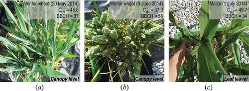
The investigated crop types are winter wheat (Triticum aestivum) and maize (Zea mays). Phenological development stages were classified according to the internationally acknowledged BBCH (Biologische Bundesanstalt, Bundessortenamt und CHemische Industrie) classification system (Meier 2011). During the first measuring day (20 May 2014) the winter wheat canopy was in the late phenological stage of stem elongation (BBCH 37, see Figure 1(a)) and irrigation had been adequately provided in the preceding days. On 9 June 2014, measurements were repeated on the winter wheat test canopy, when phenology already had progressed to the growth of panicles (BBCH 55, see Figure 1(b)). In contrast to the measurements on 20 May, irrigation had not been provided for five days before the second measuring day, despite high mid-summer air temperatures. This was done to create conditions for a heat/water stress experiment. On 1 July 2014, finally a third field experiment was realized, this time on maize. In contrast to the winter wheat canopy measurements, maize was only sampled at leaf level to avoid soil background problems within the recorded spectral signatures due to the early development stage of the maize plants (shoot development, BBCH 34, see Figure 1(c)). No apparent limitations for photosynthesis were present during the maize experiment on 1 July.

Figure 1. Vertical photographs of agricultural crop canopies examined during the 2014 growing season. Phenological status was determined according to the international BBCH scale (Meier 2011) and mean chlorophyll contents (C_chl) were derived using a Konica Minolta SPAD-502Plus device.

2.1. Measurement and analysis of high-resolution spectral signatures

2.1.1. Radiance measurements

High spectral resolution radiance measurements used to determine SIF were acquired using a calibrated ASD FieldSpec^®4 Standard-Res Spectroradiometer, with 3 nm visible and near-infrared (VNIR) resolution at full width half maximum (at 700 nm) and 1.4 nm sampling interval for the spectral region from 350 to 1000 nm. The VNIR detector consists of a 512 element silicon photo-diode array and Noise Equivalent Radiance is specified with 1.0 × 10⁻⁹ W cm⁻² nm⁻¹ sr⁻¹ at 700 nm (Analytical Spectral Devices, Inc.; Boulder, CO).

For canopy measurements the instrument’s fibre optic was attached to a swivelling mount that was elevated approximately 50 cm above the plant’s surface level and adjusted for nadir view targeting always on exactly the same canopy area. Therefore, footprint diameter was approximately 22 cm in consideration of the instrument’s field of view of 25°. The spectral measurements thus covered the entire canopy section where the vertical transects of sunlit and shaded stomatal conductance had been sampled. Leaf-level measurements were conducted using the same methodology, but with a sensor–leaf distance of approximately 9 cm. Solar irradiance measurements were acquired using a highly homogeneously reflecting calibrated Lambertian reference target (Spectralon^®, Labsphere). To avoid errors arising from significant changes in the prevailing atmospheric conditions, the respective measurements above the calibrated reference panel and vegetation samples were taken with maximum time offsets of 60 s. To ensure high-quality spectral data, 10 consecutive spectra were internally averaged as a single spectrum at each acquisition. In general, spectral measurements were taken under 100% cloud-free conditions.

2.1.2. Reflectance-based derivations

Supplementary to SIF and F_fraction, we extracted PRI and curvature performance information from the high-resolution spectral reflectance measurements.

The calculation of the PRI was performed as proposed by Gamon et al. (1990) using the reflectance (R) at 531 nm (R₅₃₁) and the xanthophyll-insensitive band at 570 nm (R₅₇₀) according to Equation (1):

(1) $\mathrm{P}\mathrm{R}\mathrm{I}= \frac{R_{531}- R_{570}}{R_{531}+ R_{570}}.$(1)

Additionally, derivative information was used to account for subtle changes in leaf and canopy reflectance that are induced by chlorophyll infilling within the O₂-A spectral region. Figure 2 illustrates the high sensitivity of the first (a) and second (b) derivative of the canopy reflectance within the O₂-A absorption range. In particular, relative high curvatures are apparent in Figure 2(b) at 760 and 762 nm. They represent the neighbouring values at both sides of the small reflectance peak induced by line infilling by chlorophyll fluorescence at 761 nm.

Figure 2. Exemplary presentation of the first (a) and second (b) derivative of a winter wheat canopy reflectance spectrum (instrument: ASD FieldSpec4 standard, acquisition date: 20 May 2014).

In this study, we investigated the capability of the second derivative of the reflectance at 760 nm (S₇₆₀) to account for fluorescence effects on canopy or leaf reflectance. Since the second derivative of the reflectance (S_λ) represents the derivative of slopes of the reflectance at the wavelength position λ, S₇₆₀ should be specifically sensitive to variations of the small reflectance peak induced by line infilling due to SIF. Calculations of derivatives are performed using finite approximation. The first derivative of the reflectance (F_λ) is estimated by Equation (2) and S_λ is derived from Equation (3):

(2) $F_{\lambda }=\frac{\mathrm{d}R}{\mathrm{d}\lambda }= \frac{R_{\lambda +1}- R_{\lambda }}{\mathrm{\Delta }\lambda },$(2)

(3) $S_{\lambda }=\frac{{\mathrm{d}}^{2}R}{\mathrm{d}{\lambda }^2}=\frac{\mathrm{d}}{\mathrm{d}\lambda }\left(\frac{\mathrm{d}R}{\mathrm{d}\lambda }\right)=\frac{R_{\lambda +2}-2R_{\lambda +1}+R_{\lambda }}{{\left(\mathrm{\Delta }\lambda \right)}^2},$(3)

where $F_{\lambda }$ is the first derivative of the reflectance between wavelength λ and λ + 1; $S_{\lambda }$ is the second derivative of the reflectance between wavelength λ and λ + 2; $R_{\lambda }$, $R_{\lambda +1}$, $R_{\lambda +2}$ is reflectance value at $\lambda$, $\lambda$ +1, $\lambda$ +2; $\mathrm{\Delta }\lambda$ is separation between adjacent bands.

Since derivatives of second order or higher are considered to be relatively insensitive to variations in illumination intensity, as stated by Tsai and Philpot (1998), no normalization was applied to S₇₆₀.

2.1.3. Applying FLD approaches

To quantify SIF emissions from high-resolution field radiance measurements, the well-proven FLD approach (Meroni et al. 2009) was applied. The FLD concept allows separating SIF emissions from the radiation reflected within dark lines of the incident solar radiation, which overlap with the red and far-red spectral region of SIF emissions. This allows quantifying the infilling due to SIF by measuring the absorption line depth of a fluorescing surface in comparison to that in the solar irradiance spectrum, which is not influenced by fluorescence. Prerequisites for applying this method are measurements inside and near the absorption line of both, incident irradiance and target radiance.

We employed the atmospheric absorption band of O₂-A to quantify the infilling effect by SIF, since it is the deepest absorption feature that overlaps with the chlorophyll fluorescence emission spectrum. Two different FLD approaches were applied, i.e. the standard FLD and the 3FLD method (Meroni et al. 2009). The wavelength used to account for the radiance and irradiance fluxes inside the O₂-A absorption feature is 761 nm for both methods, whereas method-dependent differences exist for defining the outside wavelengths on the shoulder regions of the O₂-A line. The standard FLD method only considers the left shoulder region (750–755 nm for this study), whereas the 3FLD methods accounts for both shoulder sides of the O₂-A line (in this study: 750–755 nm and 770–785 nm). Following Meroni et al. (2009), radiance (L) and irradiance (E) values inside the O₂-A line (L_in and E_in) and the previously described FLD-method-dependent values at nearby wavelengths outside the O₂-A line (L_out and E_out) were used to quantify the magnitude of SIF at 761 nm according to Equation (4):

(4) $\mathrm{S}\mathrm{I}\mathrm{F}=\frac{E_{\mathrm{o}\mathrm{u}\mathrm{t}}{L}_{\mathrm{i}\mathrm{n}}-E_{\mathrm{i}\mathrm{n}}{L}_{\mathrm{o}\mathrm{u}\mathrm{t}}}{E_{\mathrm{o}\mathrm{u}\mathrm{t}}-E_{\mathrm{i}\mathrm{n}}}.$(4)

To account for the dependency of fluorescence flux to the amount of absorbed energy potentially available for photosynthesis, adequate normalization is required. The fluorescence yield (ϕ_f) concept is frequently described in the literature (Baker 2008; Demmig and Björkman 1987; Porcar-Castell et al. 2014), where the SIF signal is related to APAR, as written in Equation (5):

(5) ${\varphi }_{\mathrm{f}}=\frac{\mathrm{S}\mathrm{I}\mathrm{F}}{\mathrm{A}\mathrm{P}\mathrm{A}\mathrm{R}}.$(5)

However, the accurate determination of APAR has proved problematic, as APAR is highly affected by the canopy structure and by the illumination geometry (Daumard et al. 2010). In this study, therefore, an easily applicable approach was applied to account for varying illumination conditions. As proposed by Daumard et al. (2010), APAR was replaced by the mean of the target radiation flux in the red spectral subsection (L_655–665) to account for changes in light interception, since chlorophylls strongly absorb in the red spectral region. By this modification the fluorescence fraction (F_fraction) variable, as written in Equation (6), should be highly related to ϕ_f.

(6) $F_{\mathrm{f}\mathrm{r}\mathrm{a}\mathrm{c}\mathrm{t}\mathrm{i}\mathrm{o}\mathrm{n}}= \frac{\mathrm{S}\mathrm{I}\mathrm{F}}{\overline{L_{655-665}}}\times 100.$(6)

However, magnitudes of F_fraction and ϕ_f are not comparable, since the respective reference values used for normalization might considerably differ from each other. For this reason, ϕ_f cannot excel the value of 1, whereas F_fraction can reach much higher numerical values.

2.2. Stomatal conductance measurements

Data on stomatal conductance (g_s) were derived by means of a handheld leaf porometer of the type SC-1 (Decagon Devices, Inc.). Porometry was conducted nearly parallel to the spectral measurements. The SC-1 instrument determines g_s by putting the conductance of a leaf in series with two known conductance elements and by comparing the humidity measurements between them. The measurement range, as stated by the manufacturer, is from 0 to 1000 mmol m⁻² s⁻¹ with an accuracy of 10% (Decagon Devices 2011). According to Pietragalla and Pask (2012) typical values for irrigated samples range between 300 and 700 mmol m⁻² s⁻¹ and for mildly water stressed leaf samples from 80 to 300 mmol m⁻² s⁻¹. Aiming for most accurate measurements of g_s, the SC-1 leaf porometer was calibrated on each measuring day and additionally was recalibrated, if the temperature and humidity conditions changed significantly during the course of the day.

In contrast to leaf area index or chlorophyll content measurements, there is no comprehensive knowledge about g_s canopy level sampling strategies. Therefore, numerous pre-tests were conducted in the context of this study to develop a sampling scheme, which accounts for the variability of g_s within geometrically complex agricultural canopies. Figure 3 shows pre-test results, where a high variability of g_s within a winter wheat canopy is observed. Distinctive differences are apparent between sunlit and shaded leaves as well as between the upper and lower layers of the winter wheat canopy. On average, values of g_s observed on sunlit leaf surfaces are higher by a factor of 2.5 compared to measured values on shaded leaves for the shown example.

Figure 3. Values of g_s (mmol m⁻² s⁻¹) observed in a winter wheat canopy in May 2014. A vertical trend of increasing g_s towards the top layer of the canopy can be observed as well as strong differences between sunlit and shaded areas.

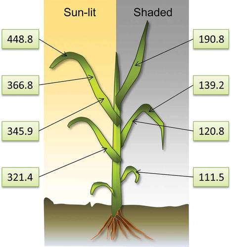
Based on these findings, a sampling strategy was applied, which meets the requirements of a representative selection of sunlit/shaded and upper/lower sample leaves on the one hand and at the same time is applicable in the field with respect to the required time effort on the other. In practice, the percentage of shaded leaf surface was estimated. Ten measurements were then distributed to sunlit and shaded leaves in accordance with this estimation. Thereby, the measurements were conducted following a vertical line starting at the bottom and ending at the top layer of the canopy in order to gauge the average canopy-level g_s. To exclude variations caused by leaf internal variability of g_s, measurements were repeatedly conducted exactly at the same marked leaf sections. However, absolute values of g_s could be biased, since full canopy representation by conducted sample measurements cannot be guaranteed. No conductance measurements were performed on stem material within the investigated canopy. Additionally, SC-1 measurements provide information about leaf temperature, which is valuable information when interpreting time series of g_s in terms of heat stress.

3. Results

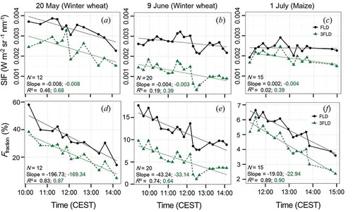
Diurnal variations of SIF and corresponding values of F_fraction are shown in Figure 4. Here, both SIF and F_fraction decrease over time in each time series presented. Differences between F_fraction retrievals are particularly noticeable when comparing the respective daily magnitudes in Figure 4(d–f). Distinct offsets are also evident between FLD and 3FLD retrievals, clearly recognizable by consistently higher FLD-based estimates compared to 3FLD estimates (please also see Section 5). However, in terms of the coefficient of determination (R²), only minor method-dependent differences of diurnal variations in SIF and F_fraction are apparent (0.59 < R² < 0.72 for SIF and 0.93 < R² < 0.99 for F_fraction between FLD and 3 FLD).

Figure 4. Derived time series of SIF (top) and F_fraction (bottom) derived from the FLD (black solid line with circles) and 3FLD (green dashed line with triangles) methods. Corresponding diurnal trends are indicated by solid lines. The first value of slope and R² (black) refers to estimates based on the standard FLD approach and the second (green) on 3FLD derived estimates of SIF and F_fraction.

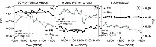
Derived time series of PRI and S₇₆₀ are presented in Figure 5. It is shown that S₇₆₀ decreases during the course of each day, especially during the winter wheat canopy experiment conducted on 20 May (a) and during the maize leaf level experiment conducted on 1 July (c). Significant differences are found between S₇₆₀ and PRI diurnal regimes, since PRI data indicate fairly stable values for all three dates. PRI values close to zero were derived on 20 May (a) and 1 July (c), where no limitations for photosynthetic processes were existent, while PRI remained low (about −0.04) during the heat and water stress experiment on 9 June (b).

Figure 5. Time series of PRI (black) and S₇₆₀ (grey). Corresponding diurnal trends are indicated by solid lines. The first value of slope and R² (black) refers to the PRI and the second (grey) to S₇₆₀.

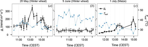
Time series derived for g_s and mean leaf temperatures T_leaf reveal varying physiological conditions for photosynthesis in between the days as shown in Figure 6. On 9 June, canopy mean g_s remained low (<72 mmol m⁻² s⁻¹) with comparably small diurnal variations (b). In the course of this day, maximum T_leaf recorded was 50.2°C with minimum values still above 30.0°C. In contrast, distinct diurnal variations in g_s were observed on 20 May (a) and 1 July (c), with considerably lower T_leaf of 29.3–39.3°C and 25.8–37.3°C, respectively. On 20 May, g_s reaches a clear maximum at 13:20 pm (343 mmol m⁻² s⁻¹) with low values at the beginning and end (108 and 100 mmol m⁻² s⁻¹) of this measurement series (a). In contrast, on 1 July, g_s increased during the measuring period from 18 to 196 mmol m⁻² s⁻¹ (c). It should be noted that the time series shown in Figure 6 covers an extended period of time compared to the time series presented in Figures 4 and 5. This results from the independency of g_s measurements from irradiative conditions (clouds, solar zenith angle). Hence, time series measurements for g_s were partly continued, even when spectral measurements had to be abandoned because of commencing cloud coverage.

Figure 6. Diurnal variations in stomatal conductance (g_s) and T_leaf derived from the SC-1 instrument. Variability of data is indicated by error bars representing one standard deviation.

4. Discussion

Independent from the applied method (FLD and 3FLD), our results indicate that during the courses of the three measuring days the amount of chlorophyll-a excitation energy dissipating as SIF decreased.

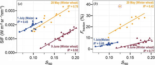
Of particular note is the similarity in the patterns of diurnal variations in S₇₆₀ to those in F_fraction and SIF (Figure 7), with S₇₆₀ largely being able to account for variations of 3FLD-based estimations of both SIF and F_fraction (0.42 ≤ R² ≤ 0.92). The good correspondence between the FLD-based results and S₇₆₀ can be traced back to the very similar calculation basis of both approaches as applied in this study. While the FLD approach directly quantifies the fluorescence infilling in the O₂-A feature at 761 nm, S₇₆₀ measures the infilling effect on the reflectance signal at 760 nm. However, weaker relationships of S₇₆₀ to F_fraction are recognizable on 20 May with R² being 0.42. This comparably weaker correlation is predominantly caused by one specific outlier highlighted in Figure 7(b). This outlier was caused by an alteration of the target radiance between 655 and 665 nm used in the described normalization scheme for F_fraction retrievals in Equation (6). Deviations of this kind can, for example, be traced to wind-induced movements of the leaves and must be expected when measuring canopies under open sky conditions (excluding the outlier highlighted in Figure 7(b) increases R² from 0.42 to 0.81).

Figure 7. Relationships between 3FLD based SIF and F_fraction retrievals to S₇₆₀. The individual measurement days are indicated by different colours.

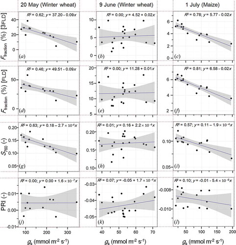
Likewise, striking is the significant relationship between diurnal measurements of g_s to F_fraction and S₇₆₀, which can be detected in our data for the experiments under unstressed conditions on 20 May and 1 July (see Figure 8). On these two days, 3FLD-based estimates of F_fraction could explain 62% (a) and 78% (c) of the variability of g_s, (p = 0.002 and p < 0.001), whereas R² values between FLD-based estimates and g_s are 0.46 (p = 0.015) for 20 May (d) and 0.81 (p < 0.001) for 1 July (f). S₇₆₀ could likewise explain variations of g_s on 20 May (g) and 1 July (i) with R² = 0.63 (p = 0.002) and 0.57 (p < 0.001). In all of these cases, negative slopes indicate inverse relationships of S₇₆₀ and F_fraction to g_s, respectively. In contrast, no correlations at all (R² ≤ 0.07) between F_fraction, S₇₆₀, and PRI to g_s were observed during the heat and water stress experiment on 9 June (e, h, k), where photosynthetic limitations are reflected by constantly low g_s and PRI values during the measurement period. In this specific case, constantly negative PRI values are an indication that the canopy is exposed to excess of light throughout the day and therefore NPQ continuously occurs. By comparison, PRI values close to zero and maximum g_s larger than 195 mmol m⁻² s⁻¹ are indications for more favourable conditions for photosynthesis on the two other days. On these days, PRI values are as constantly as expected, since initiation of NPQ to dissipate excess energy was not necessary in both cases. This also resulted in no variations of the de-epoxidation state of the xanthophyll cycle.

Figure 8. Relationships between 3FLD and FLD derived SIF, S₇₆₀ and PRI to diurnal measurements of g_s. Shaded areas represent the 95% confidence interval. It should be noted that y-axis ranges differ between the three days.

As can be seen from Figure 8(a–f), relationships between g_s and F_fraction turned out to be highly individual among the three measuring days. Possible explanations for this may be found in different states of photochemistry and heat dissipation or might be attributed to different crop types, phenology, viewing angles, or observation levels. In particular, phenological development between day 1 and day 2 (from BBCH 37 to 55) has to be considered when comparing both days, since here the same winter wheat canopy had been investigated. When interpreting the results achieved on 9 June relative to the earlier unstressed date on 20 May it therefore has to be taken into account that effects of crop development might be confounded with fluorescence plant stress response. However, the non-existent relationships between g_s and F_fraction one 9 June apparent in Figure 8(b,e) are very likely attributed to increasing non-photochemical protection in terms of heat dissipation, whereby the interrelation between photochemical light utilization and parameters related to fluorescence quantum yield is disturbed. Results are, therefore, consistent with recent findings from Van der Tol et al. (2014), highlighting the predominance of non-photochemical quenching for dissipation of excess excitation energy.

Nevertheless, the observed high diurnal variability of SIF raises the question of how single satellite observations in weekly or monthly intervals can be utilized for vegetation monitoring and modelling. Utilization of SIF retrievals for sure requires additional knowledge about potential limitations for photosynthesis, e.g. temperature and PRI measurements. This leads to the need for approaches aiming for multi-sensor data assimilation and integrated use of remote-sensing observations for fluorescence and photosynthetic modelling. Recent and promising developments in this context have been achieved in the frame of the SCOPE (Soil-Canopy Observation, Photosynthesis and Energy Balance) model, a coupled leaf physiological and radiative transfer of reflected and emitted radiation model (Van der Tol et al. 2014; van der Tol, Verhoef, and Rosema 2009; Verrelst et al. 2015). Furthermore, in order to make the best possible use of remotely sensed fluorescence data, the interchange between photosynthesis models and satellite observations should be achieved on hourly instead of daily (or even monthly) time steps, like for example realized by Hank, Bach, and Mauser (2015).

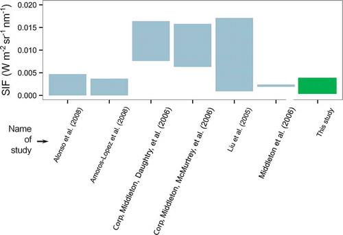
The results presented in this study so far do not allow conclusions about whether the order of magnitude of SIF retrieved from the examined winter wheat canopies and maize leaves lies within a realistic value range. Therefore, the results were compared to the range of SIF variations reported by other studies. Figure 9 gives a selection of experiments providing estimates on SIF quantified in absolute units. To allow comparability to the results of this study, only experiments that were based on the O₂-A absorption line and on measurements of the ASD device were selected. However, different vegetation types, illumination conditions, and experimental designs must still be considered between the different studies combined in Figure 9. Reported values of SIF vary from nearly zero to 0.017 W m⁻² sr⁻¹ nm⁻¹, but with significant differences among the individual studies. The highest values of SIF are reported by Liu et al. (2005) for a diurnal experiment on winter wheat. Very low values are reported by Amoros-Lopez et al. (2008) and Alonso et al. (2008) for leaf level experiments of different species exposed to high light and heat stress. SIF values presented in this article are inclined towards the lower levels of presented literature values.

Figure 9. Display of ranges of reported SIF emission values quantified within the O₂-A absorption band. Only estimates are displayed, which, comparably to this study, are based on ASD FieldSpec measurements. The value range observed in this study is highlighted in green.

5. Conclusions

In this study, diurnal measurements of SIF and g_s were performed to extend and strengthen the current knowledge about SIF variations and their dependency to different environmental conditions and daytimes. The analysis of presented time series has shown that diurnal variations of F_fraction are inversely related to g_s activity during the experiments conducted under unstressed conditions. Within a heat and water stress experiment, however, no correlation between these variables could be observed, which might be attributed to increasing photorespiration during that day. Our results thereby give insights into the complexity of interpreting SIF measurements with respect to vegetation monitoring. Nevertheless, the dependency of SIF to gas exchange rates observed in leaves and canopies under unstressed conditions emphasizes the potential use of SIF observations for vegetation monitoring purposes. Since this study is based on only three days of measurement, results may only be interpreted as a demonstration of possible relationship responses with respect to stressed and unstressed conditions. Exploiting spectral reflectance using the narrow-band spectral index PRI could provide additional information about photo-protective xanthophyll cycle dynamics and therefore allows a better interpretation of SIF measurements. Furthermore, the novel approach of using second derivative reflectance analysis at 760 nm (S₇₆₀) showed promising results for SIF estimations from hyperspectral reflectance measurements on three different days under different environmental conditions. A further analysis of the second derivative of the reflectance in SIF influenced spectral regions on larger field measurement series is necessary to assess the approach and its potential as an alternative for radiance based SIF estimations.

With respect to the choice of FLD methods our study confirms results from Damm et al. (2011), according to which the standard FLD approach may overestimate SIF if compared to the 3FLD method. However, it is important to note that our ASD FieldSpec^®4 Standard-Res Spectroradiometer measurements might overestimate true SIF values due to the relative width of the sensor FWHM and that of the O₂-A absorption line as has been demonstrated by Julitta et al. (2016).

Recently, also more sophisticated SIF retrieval methods have been developed, e.g. spectral fitting techniques (Mazzoni et al. 2012). However, exploiting these approaches requires ultra-high resolution measurements (<0.2 nm), which are seldom available. We believe that current mechanistic process understanding of SIF and of its relationship to photosynthesis-related parameters under different environmental conditions needs to be widened. The presented study, which is based on a less sophisticated but more easily applicable retrieval method, should be understood as one small step into that direction. Continued field data collection efforts, investigating both diurnal and seasonal dynamics, are recommended to enhance our mechanistic understanding of remotely sensed SIF signals, whose availability might rapidly increase with the implementation of satellite-based high spectral resolution and SIF detection capable Earth Observation Systems.

Acknowledgments

This work was supported by the space agency of the German Aerospace Center (DLR) through funding of the German Federal Ministry of Economics and Technology under the grant code 50 EE 0922.

Disclosure statement

No potential conflict of interest was reported by the authors.

Additional information

Funding

This work was supported by the space agency of the German Aerospace Center (DLR) through funding of the German Federal Ministry of Economics and Technology under the grant code [50 EE 0922].

References

- Adams, W. W., and B. Demmig-Adams. 2004. “Chlorophyll Fluorescence as a Tool to Monitor Plant Response to the Environment.” In Chlorophyll a Fluorescence, edited by G. C. Papageorgiou and G. Govindjee, 583–604. Netherlands: Springer.
- Alonso, L., L. Gomez-Chova, J. Vila-Frances, J. Amoros-Lopez, L. Guanter, J. Calpe, and J. Moreno. 2008. “Improved Fraunhofer Line Discrimination Method for Vegetation Fluorescence Quantification.” IEEE Geoscience and Remote Sensing Letters 5 (4): 620–624. doi:10.1109/LGRS.2008.2001180.
- Amoros-Lopez, J., L. Gomez‐Chova, J. Vila‐Frances, L. Alonso, J. Calpe, J. Moreno, and S. del Valle‐Tascon. 2008. “Evaluation of Remote Sensing of Vegetation Fluorescence by the Analysis of Diurnal Cycles.” International Journal of Remote Sensing 29 (17–18): 5423–5436. doi:10.1080/01431160802036391.
- Baker, N. R. 2008. “Chlorophyll Fluorescence: A Probe of Photosynthesis In Vivo.” Annual Review of Plant Biology 59 (1): 89–113. doi:10.1146/annurev.arplant.59.032607.092759.
- Buschmann, C. 1986. “Fluoreszenz-und Wärmeabstrahlung bei Pflanzen.” Die Naturwissenschaften 73 (12): 691–699. doi:10.1007/BF00399235.
- Campbell, P., E. Middleton, L. Corp, and M. Kim. 2008. “Contribution of Chlorophyll Fluorescence to the Apparent Vegetation Reflectance.” Science of the Total Environment 404 (2–3): 433–439. doi:10.1016/j.scitotenv.2007.11.004.
- Corp, L., E. Middleton, C. Daughtry, and P. E. Campbell. 2006. “Solar Induced Fluorescence and Reflectance Sensing Techniques for Monitoring Nitrogen Utilization in Corn.” Paper presented at the Geoscience and Remote Sensing Symposium, 2006. IGARSS 2006. IEEE International Conference, Denver, CO, July 31–August 4.
- Corp, L. A., E. M. Middleton, J. E. McMurtrey, P. K. E. Campbell, and L. M. Butcher. 2006. “Fluorescence Sensing Techniques for Vegetation Assessment.” Applied Optics 45 (5): 1023–1033. doi:10.1364/AO.45.001023.
- Damm, A., A. Erler, W. Hillen, M. Meroni, M. E. Schaepman, W. Verhoef, and U. Rascher. 2011. “Modeling the Impact of Spectral Sensor Configurations on the FLD Retrieval Accuracy of Sun-Induced Chlorophyll Fluorescence.” Remote Sensing of Environment 115 (8): 1882–1892. doi:10.1016/j.rse.2011.03.011.
- Daumard, F., S. Champagne, A. Fournier, Y. Goulas, A. Ounis, J.-F. Hanocq, and I. Moya. 2010. “A Field Platform for Continuous Measurement of Canopy Fluorescence.” IEEE Transactions on Geoscience and Remote Sensing 48 (9): 3358–3368. doi:10.1109/TGRS.2010.2046420.
- Demmig, B., and O. Björkman. 1987. “Comparison of the Effect of Excessive Light on Chlorophyll Fluorescence (77K) and Photon Yield of O2 Evolution in Leaves of Higher Plants.” Planta 171 (2): 171–184. doi:10.1007/BF00391092.
- Devices, D. 2011. Leaf Porometer Operators’s Manual Version 7. Pullman, WA: Decagon Devices.
- Edwards, G. E., and N. R. Baker. 1993. “Can CO2 Assimilation in Maize Leaves Be Predicted Accurately from Chlorophyll Fluorescence Analysis?.” Photosynthesis Research 37 (2): 89–102. doi:10.1007/BF02187468.
- Evain, S., J. Flexas, and I. Moya. 2004. “A New Instrument for Passive Remote Sensing: 2. Measurement of Leaf and Canopy Reflectance Changes at 531 Nm and Their Relationship with Photosynthesis and Chlorophyll Fluorescence.” Remote Sensing of Environment 91 (2): 175–185. doi:10.1016/j.rse.2004.03.012.
- Frankenberg, C., J. B. Fisher, J. Worden, G. Badgley, S. S. Saatchi, J.-E. Lee, G. C. Toon, et al. 2011. “New Global Observations of the Terrestrial Carbon Cycle from GOSAT: Patterns of Plant Fluorescence with Gross Primary Productivity.” Geophysical Research Letters 38: 17. doi:10.1029/2011GL048738.
- Gamon, J., C. Field, W. Bilger, O. Björkman, A. Fredeen, and J. Peñuelas. 1990. “Remote Sensing of the Xanthophyll Cycle and Chlorophyll Fluorescence in Sunflower Leaves and Canopies.” Oecologia 85 (1): 1–7. doi:10.1007/BF00317336.
- Garbulsky, M. F., J. Peñuelas, J. Gamon, Y. Inoue, and I. Filella. 2011. “The Photochemical Reflectance Index (PRI) and the Remote Sensing of Leaf, Canopy and Ecosystem Radiation Use Efficiencies: A Review and Meta-Analysis.” Remote Sensing of Environment 115 (2): 281–297. doi:10.1016/j.rse.2010.08.023.
- Genty, B., J.-M. Briantais, and J. B. V. Da Silva. 1987. “Effects of Drought on Primary Photosynthetic Processes of Cotton Leaves.” Plant Physiology 83 (2): 360–364. doi:10.1104/pp.83.2.360.
- Guan, K., J. A. Berry, Y. Zhang, J. Joiner, L. Guanter, G. Badgley, and D. B. Lobell. 2015. “Improving the Monitoring of Crop Productivity Using Spaceborne Solar-Induced Fluorescence.” Global Change Biology n/a-n/a. doi:10.1111/gcb.13136.
- Guanter, L., C. Frankenberg, A. Dudhia, P. E. Lewis, J. Gómez-Dans, A. Kuze, H. Suto, and R. G. Grainger. 2012. “Retrieval and Global Assessment of Terrestrial Chlorophyll Fluorescence from GOSAT Space Measurements.” Remote Sensing of Environment 121: 236–251. doi:10.1016/j.rse.2012.02.006.
- Hank, T. B., H. Bach, and W. Mauser. 2015. “Using a Remote Sensing-Supported Hydro-Agroecological Model for Field-Scale Simulation of Heterogeneous Crop Growth and Yield: Application for Wheat in Central Europe.” Remote Sensing 7 (4): 3934–3965. doi:10.3390/rs70403934.
- Joiner, J., L. Guanter, R. Lindstrot, M. Voigt, A. P. Vasilkov, E. M. Middleton, K. F. Huemmrich, Y. Yoshida, and C. Frankenberg. 2013. “Global Monitoring of Terrestrial Chlorophyll Fluorescence from Moderate Spectral Resolution Near-Infrared Satellite Measurements: Methodology, Simulations, and Application to GOME-2.” Atmospheric Measurement Techniques Discussions 6 (2): 3883–3930. doi:10.5194/amtd-6-3883-2013.
- Joiner, J., Y. Yoshida, A. Vasilkov, Y. Yoshida, L. A. Corp, and E. M. Middleton. 2011. “First Observations of Global and Seasonal Terrestrial Chlorophyll Fluorescence from Space.” Biogeosciences 8 (3): 637–651. doi:10.5194/bg-8-637-2011.
- Julitta, T., L. Corp, M. Rossini, A. Burkart, S. Cogliati, N. Davies, M. Hom, et al. 2016. “Comparison of Sun-Induced Chlorophyll Fluorescence Estimates Obtained from Four Portable Field Spectroradiometers.” Remote Sensing 8 (2): 122. doi:10.3390/rs8020122.
- Krause, G. H., and E. Weis. 1984. “Chlorophyll Fluorescence as a Tool in Plant Physiology.” Photosynthesis Research 5 (2): 139–157. doi:10.1007/BF00028527.
- Lee, J.-E., C. Frankenberg, C. van der Tol, J. A. Berry, L. Guanter, C. K. Boyce, J. B. Fisher, et al. 2013. “Forest Productivity and Water Stress in Amazonia: Observations from GOSAT Chlorophyll Fluorescence.” Proceedings of the Royal Society of London B: Biological Sciences 280 (1761): 20130171. doi:10.1098/rspb.2013.0171.
- Liu, L., Y. Zhang, J. Wang, and C. Zhao. 2005. “Detecting Solar-Induced Chlorophyll Fluorescence from Field Radiance Spectra Based on the Fraunhofer Line Principle.” IEEE Transactions on Geoscience and Remote Sensing 43 (4): 827–832. doi:10.1109/TGRS.2005.843320.
- Louis, J., A. Ounis, J.-M. Ducruet, S. Evain, T. Laurila, T. Thum, M. Aurela, et al. 2005. “Remote Sensing of Sunlight-Induced Chlorophyll Fluorescence and Reflectance of Scots Pine in the Boreal Forest during Spring Recovery.” Remote Sensing of Environment 96 (1): 37–48. doi:10.1016/j.rse.2005.01.013.
- Malenovky, Z., A. Ac, J. Olejnickova, A. Galle, U. Rascher, and G. Mohammed. 2014. “Knowledge Gap Analysis Assessing Steady-State Chlorophyll Fluorescence as an Indicator of Plant Stress Status.” Paper presented at the proceedings of the 5th international workshop on Remote Sensing of Vegetatin Fluorescence, Paris, 2014 April 22–24.
- Mazzoni, M., M. Meroni, C. Fortunato, R. Colombo, and W. Verhoef. 2012. “Retrieval of Maize Canopy Fluorescence and Reflectance by Spectral Fitting in the O2–A Absorption Band.” Remote Sensing of Environment 124: 72–82. doi:10.1016/j.rse.2012.04.025.
- Meier, U. 2011. Growth Stages of Mono-And Dicotyledonous Plants. BBCH Monograph. 2nd ed. Federal Biological Research Centre for Agriculture and Forestry. http://www.jki.bund.de/fileadmin/dam_uploads/_veroeff/bbch/BBCH-Skala_englisch.pdf
- Meroni, M., and R. Colombo. 2006. “Leaf Level Detection of Solar Induced Chlorophyll Fluorescence by Means of a Subnanometer Resolution Spectroradiometer.” Remote Sensing of Environment 103 (4): 438–448. doi:10.1016/j.rse.2006.03.016.
- Meroni, M., M. Rossini, L. Guanter, L. Alonso, U. Rascher, R. Colombo, and J. Moreno. 2009. “Remote Sensing of Solar-Induced Chlorophyll Fluorescence: Review of Methods and Applications.” Remote Sensing of Environment 113 (10): 2037–2051. doi:10.1016/j.rse.2009.05.003.
- Middleton, E. M., L. Corp, and P. Campbell. 2008. “Comparison of Measurements and Fluormod Simulations for Solar-Induced Chlorophyll Fluorescence and Reflectance of a Corn Crop under Nitrogen Treatments.” International Journal of Remote Sensing 29 (17–18): 5193–5213. doi:10.1080/01431160802036524.
- Middleton, E. M., L. A. Corp, C. S. T. Daughtry, and P. Campbell. 2006. “Chlorophyll Fluorescence Emissions of Vegetation Canopies from High Resolution Field Reflectance Spectra.” Paper presented at the Geoscience and Remote Sensing Symposium, 2006. IGARSS 2006. IEEE International Conference on, Denver, CO, July 31–August 4.
- Ni, Z., Z. Liu, H. Huo, Z.-L. Li, F. Nerry, Q. Wang, and X. Li. 2015. “Early Water Stress Detection Using Leaf-Level Measurements of Chlorophyll Fluorescence and Temperature Data.” Remote Sensing 7 (3): 3232–3249. doi:10.3390/rs70303232.
- Pietragalla, J., and A. Pask. 2012. Physiological Breeding II: A Field Guide to Wheat Phenotyping, edited by A. J. D. Pask, J. Pietragalla, D. M. Mullan, and M. P. Reynolds. Mexico City: CIMMYT.
- Plascyk, J. A., and F. C. Gabriel. 1975. “The Fraunhofer Line Discriminator MKII-An Airborne Instrument for Precise and Standardized Ecological Luminescence Measurement.” IEEE Transactions on Instrumentation and Measurement 24 (4): 306–313. doi:10.1109/TIM.1975.4314448.
- Porcar-Castell, A., E. Tyystjärvi, J. Atherton, C. van der Tol, J. Flexas, E. E. Pfündel, J. Moreno, C. Frankenberg, and J. A. Berry. 2014. “Linking Chlorophyll a Fluorescence to Photosynthesis for Remote Sensing Applications: Mechanisms and Challenges.” Journal of Experimental Botany 65: 4065–4095. doi:10.1093/jxb/eru191.
- Raji, S. N., N. Subhash, V. Ravi, R. Saravanan, C. N. Mohanan, S. Nita, and T. M. Kumar. 2015. “Detection of Mosaic Virus Disease in Cassava Plants by Sunlight-Induced Fluorescence Imaging: A Pilot Study for Proximal Sensing.” International Journal of Remote Sensing 36 (11): 2880–2897. doi:10.1080/01431161.2015.1049382.
- Rascher, U., G. Agati, L. Alonso, G. Cecchi, S. Champagne, R. Colombo, A. Damm, et al. 2009. “CEFLES2: The Remote Sensing Component to Quantify Photosynthetic Efficiency from the Leaf to the Region by Measuring Sun-Induced Fluorescence in the Oxygen Absorption Bands.” Biogeosciences 6 (7): 1181–1198. doi:10.5194/bg-6-1181-2009.
- Richter, K., C. Atzberger, T. B. Hank, and W. Mauser. 2012. “Derivation of Biophysical Variables from Earth Observation Data: Validation and Statistical Measures.” Journal of Applied Remote Sensing 6 (1): 063557-1–063557-23. doi:10.1117/1.JRS.6.063557.
- Santrucek, J., P. Siffel, H. Synkova, V. Konecna, M. Lang, H. Lichtenthaler, C. Schindler, and K. Szabo. 1992. “Photosynthetic Activity and Chlorophyll Fluorescence Parameters in Aurea and Green Forms of Nicotiana Tabacum.” Photosynthetica 27: 529–543.
- Sayed, O. 2003. “Chlorophyll Fluorescence as a Tool in Cereal Crop Research.” Photosynthetica 41 (3): 321–330. doi:10.1023/B:PHOT.0000015454.36367.e2.
- Tsai, F., and W. Philpot. 1998. “Derivative Analysis of Hyperspectral Data.” Remote Sensing of Environment 66 (1): 41–51. doi:10.1016/S0034-4257(98)00032-7.
- Van der Tol, C., J. Berry, P. Campbell, and U. Rascher. 2014. “Models of Fluorescence and Photosynthesis for Interpreting Measurements of Solar-Induced Chlorophyll Fluorescence.” Journal of Geophysical Research: Biogeosciences 119 (12): 2312–2327.
- van der Tol, C., W. Verhoef, and A. Rosema. 2009. “A Model for Chlorophyll Fluorescence and Photosynthesis at Leaf Scale.” Agricultural and Forest Meteorology 149 (1): 96–105. doi:10.1016/j.agrformet.2008.07.007.
- Verrelst, J., J. P. Rivera, C. van der Tol, F. Magnani, G. Mohammed, and J. Moreno. 2015. “Global Sensitivity Analysis of the SCOPE Model: What Drives Simulated Canopy-Leaving Sun-Induced Fluorescence?.” Remote Sensing of Environment 166: 8–21. doi:10.1016/j.rse.2015.06.002.
- Yang, X., J. Tang, J. F. Mustard, J.-E. Lee, M. Rossini, J. Joiner, J. W. Munger, A. Kornfeld, and A. D. Richardson. 2015. “Solar-Induced Chlorophyll Fluorescence that Correlates with Canopy Photosynthesis on Diurnal and Seasonal Scales in a Temperate Deciduous Forest.” Geophysical Research Letters 42 (8): 2977–2987. doi:10.1002/2015GL063201.
- Zarco-Tejada, P. J., J. A. J. Berni, L. Suárez, G. Sepulcre-Cantó, F. Morales, and J. R. Miller. 2009. “Imaging Chlorophyll Fluorescence with an Airborne Narrow-Band Multispectral Camera for Vegetation Stress Detection.” Remote Sensing of Environment 113 (6): 1262–1275. doi:10.1016/j.rse.2009.02.016.
- Zarco-Tejada, P. J., A. Catalina, M. González, and P. Martín. 2013. “Relationships between Net Photosynthesis and Steady-State Chlorophyll Fluorescence Retrieved from Airborne Hyperspectral Imagery.” Remote Sensing of Environment 136: 247–258. doi:10.1016/j.rse.2013.05.011.
- Zarco-Tejada, P. J., V. González-Dugo, and J. A. J. Berni. 2012. “Fluorescence, Temperature and Narrow-Band Indices Acquired from a UAV Platform for Water Stress Detection Using a Micro-Hyperspectral Imager and a Thermal Camera.” Remote Sensing of Environment 117: 322–337. doi:10.1016/j.rse.2011.10.007.
- Zarco-Tejada, P. J., A. Morales, L. Testi, and F. J. Villalobos. 2013. “Spatio-Temporal Patterns of Chlorophyll Fluorescence and Physiological and Structural Indices Acquired from Hyperspectral Imagery as Compared with Carbon Fluxes Measured with Eddy Covariance.” Remote Sensing of Environment 133: 102–115. doi:10.1016/j.rse.2013.02.003.