A simplified high and near-constant contrast approach for the display of VIIRS day/night band imagery

ABSTRACT

The European Organisation for the Exploitation of Meteorological Satellites has developed a simplified high and near-constant contrast approach for the display of Day and Night Band (DNB) data of Suomi National Polar-orbiting Partnership (S-NPP) satellite’s instrument Visible Infrared Imager Radiometer Suite (VIIRS). Simple applications like service monitoring or operational weather forecasting (nowcasting) can thus take direct advantage of the VIIRS DNB Level 1 data without the need for using Level 2 processing, Level 2 data or using ancillary data like look-up tables. This method is based on a fixed ’correction curve’ and simple formulas, and can thus be applied sequentially to single granules as, e.g., received through direct broadcast dissemination systems. Especially the European Nordic Countries need to rely on good contrast imagery for operational weather forecasting during the extended twilight periods from autumn to spring.

1. Introduction

The European Organisation for the Exploitation of Meteorological Satellites (EUMETSAT) disseminates as part of its EUMETSAT Advanced Retransmission Service (EARS) Level 1 (L1) Sensor Data Records (SDR) from the Day and Night Band (DNB) of the Visible Infrared Imager Radiometer Suite (VIIRS) onboard of the Suomi National Polar-orbiting Partnership satellite (EUMETSAT 2016).

The DNB is a panchromatic channel (full width/half maximum response from 500 to 900 nm, 700 nm centre wavelength) (Miller et al. 2013), and due to its high dynamic range (3 × 10^–9 W cm⁻² sr⁻¹ – 2 × 10^–2 W cm⁻² sr⁻¹) (NASA 2014), the instrument is capable of detecting Earth scenes as dim as airglow at night to the brightest daytime solar illumination.

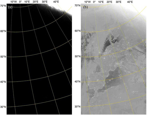
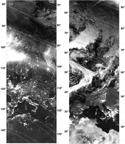
However, for reasons of this wide dynamic range, creating grey-scale images of the captured scenes, e.g. for monitoring purposes or for operational weather forecasting and nowcasting applications, is not possible without correction to the radiances: either sun-illuminated areas or areas around the terminator will be too bright or night-time areas will be too dark. A simplistic correction approach using linear or logarithmic scaling of the radiances delivers unsatisfactory results; see, e.g., Seaman and Miller (2015) and Figure 1(a ) and (b), although logarithmic scaling with manual optimization of range and contrast gives adequate results for case studies over limited areas.

Figure 1. Examples of DNB imagery using (a) a simple linear and (b) a simple logarithmic scaling for a half moon scene over Europe and North Africa collected on 25 August 2016 from 01:26:08Z to 01:38:54Z. Grid lines show the latitudes/longitudes (yellow).

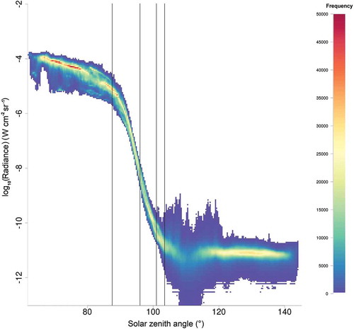
Figure 2 shows an example two-dimensional (2D) histogram of the biased radiances found in a scene (2 August 2016 from 01:51:40Z to 02:18:40Z) as a function of the sun zenith angle. The vertical black reference lines refer to the different regions of the correction curve introduced in the next section. The radiances have been biased by 2.6 × 10^–10 W cm⁻² sr⁻¹ before displaying them due to the existence of negative radiances in the L1 SDR. Please see more on this topic in the next section relating to Equation (13).

Figure 2. 2D histogram of biased radiances as a function of the sun zenith angle for a new-moon scene on 2 August 2016 from 01:51:40Z to 02:18:40Z, 256 × 256 bins. The vertical black reference lines refer to the different regions of the correction curve introduced in the next section.

The National Oceanic and Atmospheric Administration (NOAA) and the National Aeronautics and Space Administration produce Level 2 products (Environmental Data Record, EDR) of the L1 SDRs called Near-Constant Contrast (NCC) (Hillger et al. 2014) which correct for the wide range of radiances through solar/lunar-zenith-angle-dependent gain adjustments. Recently, Liang et al. (2014) documented how NCC imagery can be created for all solar and lunar conditions. While the described method provides good results, it needs specialized post-processing of the L1 SDRs using ancillary optimized look-up tables which are not directly available.

The goal is, thus, to have a simple approach using only the data provided through the L1 SDRs and without the need for ancillary data to create digital imagery with high and near-constant contrast (HNCC) for all illumination conditions at night and around the terminator regions. Especially the European Nordic Countries need to rely on good contrast imagery for operational weather forecast during the extended twilight periods from autumn to spring.

The definition of the VIIRS SDR format by NOAA includes the separation of the data in granules of approximately 85.3 s each. This scheme is also applied by EARS. The proposed approach for the display of VIIRS-DNB data shall work with the same settings for all granules. In that way, it will be transparent if the approach is applied to single granules whose images are then stitched together or applied to a concatenation of granules. This will support the use case scenario of users receiving granules with high timeliness through direct broadcast services and displaying them as soon as they are available.

2. Methods

Based on (Liang et al. 2014) and Figure 2, a simple solar and lunar-zenith-angle-dependent gain adjustment function (‘correction curve’) was developed empirically (see Figure 3).

Figure 3. Zenith-angle-dependent gain factors.

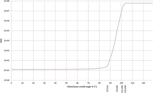
The sun and lunar zenith angle ranges are sub-divided into five regions, and the curve in Figure 3 is defined in five parts:

(1) $G\left(\theta \right)=\left\{\begin{array}{c}\frac{58+\frac{4}{\mathrm{c}\mathrm{o}\mathrm{s}\left(\theta \right)}}{5},\theta \le {87.541}^{\circ }\\ 123{\mathrm{e}}^{1.06\left(\theta -89.589\right)}\left(\frac{{\left(\theta -93\right)}^2}{18}+0.5\right),{87.541}^{\circ }<\theta \le {96.000}^{\circ }\\ 123{\mathrm{e}}^{1.06\left(\theta -89.589\right)},{96.000}^{\circ }<\theta \le {101.000}^{\circ }\\ 123{\mathrm{e}}^{1.06\left(101-89.589\right)}\mathrm{l}{\mathrm{n}}^2\left(\theta -\left(101-\mathrm{e}\right)\right),{101.000}^{\circ }<\theta \le {103.490}^{\circ }\\ 6\times {10}^7,{103.490}^{\circ }<\theta \end{array}\right.$(1)

where G is the gain factor for solar and lunar zenith angle correction and θ is the solar or lunar zenith angle in degrees; e is the Euler number.

The split in 5 zones covers the transition from the low zenith angles with a dominant cos⁻¹ dependency to the more and more refraction dominated situations where the sun (or moon) is nearer to or even below the horizon.

The gain factor G _s for the solar zenith angle θ _s is

(2) $G_{\mathrm{s}}=G\left({\theta }_{\mathrm{s}}\right).$(2)

According to (Allen 1973), the variation $V\left(\phi \right)$ of the apparent magnitude for the moon with its phase angle $\phi$ can be approximated by

(3) $V\left(\phi \right)=0.026\phi +4.0\times {10}^{-9}{\phi }^4,$(3)

and according to (Seidelmann 2006) the moon illumination fraction F _l, $F_{\mathrm{l}}\in \left[0;1\right]$ can be derived from the moon phase angle $\phi$ via

(4) $F_{\mathrm{l}}\left(\phi \right)=0.5\left[1+cos\left(\phi \right)\right].$(4)

Hence,

(5) $\phi \left(F_{\mathrm{l}}\right)=arccos\left(2F_{\mathrm{l}}-1\right),$(5)

and the variation V(F _l) of the apparent magnitude for the moon with its moon illumination fraction F _l is

(6) $V\left(F_{\mathrm{l}}\right)=0.026arccos\left(2F_{\mathrm{l}}-1\right)+4.0\times {10}^{-9}\hspace{0.17em}[arccos\left(2F_{\mathrm{l}}-1\right){]}^4.$(6)

The apparent magnitude m_s of the sun is −26.74 and the mean apparent magnitude m_l,f of the full moon is −12.74.

The apparent magnitude of the moon m _l depending on its moon illumination fraction F _l is

(7) ${\mathrm{m}}_{\mathrm{l}}\left(F_{\mathrm{l}}\right)=V\left(F_{\mathrm{l}}\right)+\hspace{0.17em}{\mathrm{m}}_{\mathrm{l},\mathrm{f}.}$(7)

We define the brightness ratio R _s,l(F _l) of the sun’s brightness b _s and the moon’s brightness b _l(F _l) as

(8) $R_{\mathrm{s},\mathrm{l}}\left(F_{\mathrm{l}}\right)=\frac{b_{\mathrm{s}}}{b_{\mathrm{l}}\left(F_{\mathrm{l}}\right)}.$(8)

Using Pogson’s law (Bishop 2016),

(9) ${\mathrm{m}}_{\mathrm{s}}-{\mathrm{m}}_{\mathrm{l}}\left(F_{\mathrm{l}}\right)=-2.5\mathrm{l}\mathrm{o}{\mathrm{g}}_{10}\left[R_{\mathrm{s},\mathrm{l}}\left(F_{\mathrm{l}}\right)\right]$(9)

we get for the brightness ratio R _s,l(F _l) of the sun and the moon

(10) $R_{\mathrm{s},\mathrm{l}}\left(F_{\mathrm{l}}\right)={10}^{\frac{{\mathrm{m}}_{\mathrm{s}}-m_{\mathrm{l}}\left(F_{\mathrm{l}}\right)}{-2.5}}.$(10)

The gain factor G _l for the lunar zenith angle θ _l and the moon illumination fraction F _l is then

(11) $G_{\mathrm{l}}=R_{\mathrm{s},\mathrm{l}}\left(F_{\mathrm{l}}\right)G\left({\theta }_{\mathrm{l}}\right).$(11)

The total gain factor G _tot applied to the radiances is

(12) $G_{\mathrm{t}\mathrm{o}\mathrm{t}}=\frac{1}{\frac{1}{G_{\mathrm{s}}}+\frac{1}{G_{\mathrm{l}}}}\hspace{0.17em}.$(12)

The radiances L in the DNB are sometimes negative due to the too large clear-sky offsets used in the DNB SDR calibration (NOAA 2015, 25).

To correct for this effect, a systematic bias for the radiances L (Liao et al. 2013, 12712) is introduced to get biased radiances L´:

(13) $L^{\prime }=L+2.6\times {10}^{-10}\mathrm{W}\mathrm{c}{\mathrm{m}}^{-2}\mathrm{s}{\mathrm{r}}^{-1}.$(13)

The normalized radiances L _norm used to display the image are

(14) $L_{\mathrm{n}\mathrm{o}\mathrm{r}\mathrm{m}}=L^{\prime }{G}_{\mathrm{t}\mathrm{o}\mathrm{t}}.$(14)

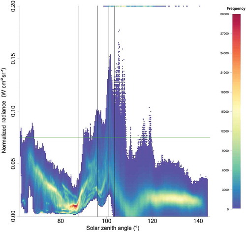
Using Equations (1–2), (6–7), and (10–14), the radiances L of the VIIRS DNB SDR are converted into normalized radiances L _norm. Empirical analysis (see, e.g., Figure 4) showed that limiting the number range of the normalized radiances to [0; 0.075] will produce the best image results in terms of contrast for all illumination conditions. The number range [0; 0.075] is then mapped to the grey-scale pixel value range [0; 255]. Values below 0 are mapped to the grey-scale pixel value 0 (black) and values above 0.075 are mapped to the grey-scale pixel value 255 (white).

Figure 4. 2D histogram of normalized radiances for the new-moon scene shown in Figure 2 (2 August 2016 from 01:51:40Z to 02:18:40Z), 256 × 256 bins. The vertical black reference lines refer to the different regions of the correction curve introduced in Equation (1). The horizontal reference line is the cut-off value of 0.075.

Please note that the applied corrections through the solar and lunar gain factors do not account for the varying sun–earth or earth–moon distances. Additionally, the dependencies on solar and lunar azimuth angles are not considered as those are believed to be negligible except for cases of sun and moon glint off reflective surfaces.

Figure 4 shows the 2D histogram of normalized radiances for the new-moon scene shown in Figure 2 (2 August 2016 from 01:51:40Z to 02:18:40Z). The vertical black reference lines refer to the different regions of the correction curve introduced in Equation (1). The green horizontal reference line is the cut-off value of 0.075. This cut-off filters, e.g., the effect of dominant city lights during night. In that way, the contrast for the desired meteorological and surface features is significantly improved.

3. Results and discussion

Figure 5(a ) shows a concatenated scene of VIIRS DNB imagery created with our simplified HNCC approach over Europe. The data were received via the EARS ground stations at Svalbard, Lannion and Athens on 1 September 2016 (new moon) from 00:44:42Z to 01:13:08Z.

Figure 5. HNCC imagery showing Europe and North Africa (a) in the night-time at new moon (1 September 2016 from 00:44:42Z to 01:13:08Z) and (b) during daytime (1 September 2016 from 12:18:53Z–12:44:28Z). Grid lines show the sun zenith angle (numbers right of images) and the moon zenith angle (numbers left of images) in degrees.

The lower part is night, in the middle upper part it is twilight, and in the upper right part it is daylight. The twilight area is very bright at certain places, created by sun glare on top of the clouds due to the very low sun elevation. This effect cannot be corrected by our simplified approach.

Figure 5(b ) shows nearly the same region roughly 12 h later (12:18:53Z–12:44:28Z). Here, we have daylight in most of the image and twilight in the uppermost right.

The images show as well grid lines for the sun zenith angle (numbers right of images) and the moon zenith angle (numbers left of images).

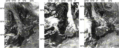
Another example in Figure 6 shows the movement of a weather system from the Atlantic Ocean over western France: (a) shows a scene on 17 August 2016 around 02:20Z (one day before full-moon), (b) roughly the same region on the same day during daylight around 13:50Z, and (c) the same region on 18 August 2016 around 02:00Z (full moon).

Figure 6. Movement of a weather system from the Atlantic Ocean over western France. (a) shows a scene on 17 August 2016 around 02:20Z (one day to full-moon), (b) roughly the same region on the same day during daylight around 13:50Z, and (c) the same region on 18 August 2016 around 02:00Z (full moon). The narrow black horizontal stripe over Great Britain and France in (a) is due to a reception dropout in the Direct Broadcast reception.

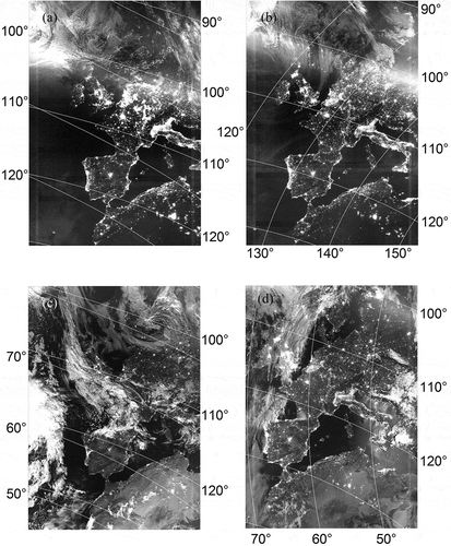
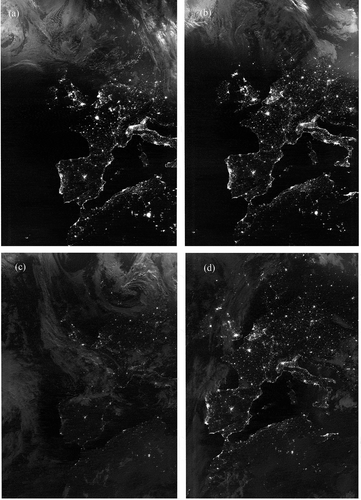
Figure 7 shows in comparison images during (a) new-moon (2 August 2016), (b) quarter-moon waxing (8 August 2016), (c) full-moon (18 August 2016), and (d) half moon waning (25 August 2016) of roughly the same region. Please note that in the quarter-moon scene (b), the moon has not risen above the horizon, yet. Note as well that the full-moon image in Figure 7(c ) is – disregarding city-lights – nearly indistinguishable from the daytime image in Figure 5(b ) in terms of illumination.

Figure 7. HNCC imagery showing Europe and North-West Africa (a) during new-moon (2 August 2016), (b) quarter-moon waxing (8 August 2016), (c) full-moon (18 August 2016), and (d) half moon waning (25 August 2016). Grid lines show the sun zenith angle (numbers right of images) and the moon zenith angle (numbers left or below of images). Note that in the quarter-moon scene (b) the moon has not risen above the horizon, yet.

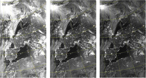
We have analysed which effect it has when using other cut-off values. When lowering the cut-off value, more regions are overexposed and darker features become more visible. When raising the cut-off value, fewer regions are overexposed and darker features become less visible.

Figure 8 shows the corrected half-moon scene of Figure 7(d ) (25 August 2016 from 01:26:08Z to 01:38:54Z) using different cut-off values: (a) 0.060, (b) 0.100 and (c) 0.140. The author is the most satisfied when using 0.075 as the cut-off value as shown in Figure 7(d ). Other users may wish to use a different cut-off value depending on their needs to highlight different features.

Figure 8. Corrected half-moon scene (25 August 2016 from 01:26:08Z to 01:38:54Z) using different cut-off values: (a) 0.060, (b) 0.100 and (c) 0.140.

3.1. Comparison with other approaches

For comparison with other approaches, we have compared the imagery created by the described simplified HNCC approach with imagery created using the operational NOAA NCC Level 2 product (Hillger et al. 2014) and with the ERF dynamic scaling function as described in Seaman and Miller (2015).

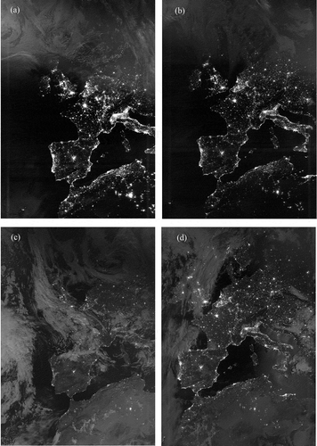
Figure 9 shows the same scenes as displayed in Figure 7 but created from the operational NCC products. The operational NCC product contains pseudo-albedo values between −10 and 1000. Following (Seaman and Miller 2015), and for better comparison, we have as well limited the pseudo-albedo values found in the product to a range from 0 to 2 and scaled those linearly.

Figure 9. Same as in Figure 7 but using NCC images.

Figure 10 shows the same scenes as well but created through the ERF dynamic scaling function as described in Seaman and Miller (2015).

Figure 10. Same as in Figure 7 but using images created through ERF dynamic scaling. Images provided by Dr Curtis Seaman.

For the new moon scene in Figure 7(a ), Figure 9(a), and Figure 10(a), the NCC approach (Figure 9) shows a better contrast in the region between 90° and 100° sun zenith angle than the ERF approach (Figure 10). Our simplified HNCC approach shows even better contrast, but is over-saturated in the upper left part. In the lower left part of the scene (around Madeira), the most cloud details are picked up by our HNCC approach, followed by the ERF approach, while the NCC approach does not show any cloud features.

For the quarter moon scene in Figure 7(b ), Figure 9(b ), and Figure 10(b ), again, the HNCC approach displays the most cloud features in comparison to the other two approaches and shows the highest and most constant contrast across the scene.

For the full moon scene in Figure 7(c ), Figure 9(c ), and Figure 10(c ), the best contrast over the whole scene is present in our simplified HNCC approach. The ERF approach compares better to the NCC approach for features with a sun zenith angle greater than approximately 100°, and the NCC approach compares better to the ERF approach for sun zenith angles smaller than approximately 100°.

For the half moon scene in Figure 7(d ), Figure 9(d ), and Figure 10(d ), the best contrast over the whole scene is again present in our simplified HNCC approach. Cloud features not or hardly visible in the other two approaches can be clearly distinguished in our approach, e.g. around the city of Minsk in Belarus.

3.2. Differences with the near constant contrast (NCC) approach

The presented HNCC approach is based on Liang et al. (2014). Thus, the following paragraphs highlight the differences between the two approaches.

With comparison to the correction curve definition of the operational NOAA NCC Level 2 product (Liang et al. 2014), we have chosen different zenith angle ranges for the piece-wise definition of the correction curve. Note that the split of the correction curve as well into five pieces is purely coincidental. Additionally, the curve beyond θ = 87.541° is not purely exponential, but empirically adapted to better fit the observed changes in radiances with the solar (and lunar) zenith angles: in the second part of the curve-definition (87.541° < θ ≤ 96°), a quadratic dependency with the zenith angle of the exponential definition is introduced, in the fourth part (101° < θ ≤ 103.49°) a dominant logarithmic influence is present, and in the fifth part (103.49° < θ) a constant value is used as no direct dependency of the observed radiances from either solar or lunar zenith angles can be seen.

The differences of the gain values for the solar and lunar components in the HNCC approach are derived from theoretical astronomical considerations, while in the NCC algorithm those were derived through the Moderate Resolution Atmospheric Transmission (MODTRAN) model. MODTRAN was as well used in the NCC approach to calculate the solar and lunar asymmetric reflectance factors, which are dependent on the solar zenith, sensor zenith and solar relative azimuth, and the lunar zenith, sensor zenith, and lunar relative azimuth angles, respectively. The sensor zenith, solar (relative) azimuth, and lunar (relative) azimuth angles are not used in the HNCC approach.

Finally, the NCC algorithm creates pseudo-albedo values rather than scaled or normalized radiances as in the HNCC or ERF approach, and the pseudo-albedo values are mapped using the ground-track Mercator algorithm, while the HNCC does not reproject the data. If needed, the HNCC data can be reprojected by the user for final display of the imagery.

The advantage of the described HNCC approach is to use only the solar and lunar zenith angles as available on a per-pixel basis of the radiance data, and the moon illumination fraction as available once for the scene within the L1 SDR product. No other ancillary data, e.g. look-up tables like in the NCC algorithm, are needed.

This simplistic HNCC approach does not account, though, for sun-glare, sun- or moon-glint, side-illumination of clouds, atmospheric scattering, straylight, or sun or moon eclipses, and does not consider the varying sun-earth or earth–moon distances. As the HNCC approach is more simple than the NCC algorithm, it cannot preserve the original image content of the data as good as in the NCC product. It is, though, well suited for fast visualisation of data as needed by, e.g., operational weather forecasters.

Another drawback of the NCC algorithm as currently available in the Community Satellite Processing Package (CSPP) for users of Direct Broadcast data is that it cannot work directly with the L1 SDR data as disseminated by Direct Broadcast retransmission systems like EARS, as the L2 EDR NCC computation in CSPP requires temporary data created during the SDR generation which are not disseminated to the users.

As shown earlier, the presented approach creates simplified high and near-constant contrast imagery for all types of daytime and night-time illumination.

Users in need of a simple and fast method to display VIIRS DNB imagery without the need for ancillary data or further product processing will benefit from the described approach.

4. Conclusion

We have presented a simplified approach of creating high and near-constant contrast imagery for VIIRS DNB data based solely on information available within the L1 SDR products, namely the sun and lunar zenith angles, and the lunar illumination fraction. The resulting imagery is suitable for simple applications such as service monitoring or operational weather forecast and nowcasting, and it compares favourably with other near constant contrast methods like the operational NCC algorithm or the ERF dynamic scaling approach. No ancillary data, e.g. in the form of lookup tables, is needed. The presented approach is not scene-optimized and as such can be applied to single granules of data for continuous display or to concatenated (aggregated) data.

Acknowledgments

The author would like to thank Dr Curtis Seaman for the provision of ERF imagery used in this article, and Dr Thomas Heinemann, Mr Anders Soerensen, Dr Dieter Klaes, Mr Hans-Peter Roesli, Mrs Ruth Weitzel, and Dr Tim Hewison for their helpful comments and assistance in preparing this article. Additionally, the author would like to thank the anonymous reviewers for their helpful suggestions and comments.

Disclosure statement

No potential conflict of interest was reported by the author.

References

- Allen, C. W. 1973. Astrophysical Quantities , 144. London: Athlone Press.
- Bishop, C. 2016. Astrophysics AQA A-Level Year 2 , 24–25. London: Collins.
- EUMETSAT (European Organisation for the Exploitation of Meteorological Satellites) . 2016. “EARS-VIIRS Service Specification.” http://www.eumetsat.int/website/home/Data/RegionalDataServiceEARS/EARSVIIRS/index.html
- Hillger, D. , C. Seaman , C. Liang , S. Miller , D. Lindsey , and T. Kopp . 2014. “Suomi NPP VIIRS Imagery Evaluation.” Journal of Geophysical Research: Atmospheres 119: 6440–6455. doi:10.1002/2013JD021170.
- Liang, C. K. , S. Mills , B. I. Hauss , and S. D. Miller . 2014. “Improved VIIRS Day/Night Band Imagery with near Constant Contrast.” IEEE Transactions on Geoscience and Remote Sensing 52 (11): 6964–6971. doi:10.1109/TGRS.2014.2306132.
- Liao, L. B. , S. Weiss , S. Mills , and B. Hauss . 2013. “Suomi NPP VIIRS Day-Night Band On-Orbit Performance.” Journal of Geophysical Research: Atmospheres 118: 12705–12718. doi:10.1002/2013JD020475.
- Miller, S. D. , W. Straka III , S. P. Mills , C. D. Elvidge , T. F. Lee , J. Solbrig , A. Walther , A. K. Heidinger , and S. C. Weiss . 2013. “Illuminating the Capabilities of the Suomi National Polar-Orbiting Partnership (NPP) Visible Infrared Imaging Radiometer Suite (VIIRS) Day/Night Band.” Remote Sensing 5 (12): 6717–6766. doi:10.3390/rs5126717.
- NASA (National Aeronautics and Space Administration) . 2014. Joint Polar Satellite System (JPSS) VIIRS Radiometric Calibration Algorithm Theoretical Basis Document (ATBD) . Greenbelt: Goddard Space Flight Center. http://npp.gsfc.nasa.gov/sciencedocs/2015-06/474-00027_ATBD-VIIRS-Radiometric-Calibration_C.pdf
- NOAA (National Oceanic and Atmospheric Administration) . 2015. “Visible Infrared Imaging Radiometer Suite (VIIRS) Imagery Environmental Data Record (EDR) User’s Guide. Version 1.3.” NOAA Technical Report NESDIS 150 . Washington, DC. doi:10.7289/V5/TR-NESDIS-150.
- Seaman, C. J. , and S. D. Miller . 2015. “A Dynamic Scaling Algorithm for the Optimized Digital Display of VIIRS Day/Night Band Imagery.” International Journal of Remote Sensing 36 (7): 1839–1854. doi:10.1080/01431161.2015.1029100.
- Seidelmann, P. K. , ed. 2006. Explanatory Supplement to the Astronomical Almanac , 396. Sausalito, CA: University Science Books.