Quantifying suspended sediment concentration in subglacial sediment plumes discharging from two Svalbard tidewater glaciers using Landsat-8 and in situ measurements

ABSTRACT

Marine-terminating outlet glaciers discharge mass through iceberg calving, submarine melting, and meltwater run-off. While calving can be quantified by in situ and remote-sensing observations, meltwater run-off, the subglacial transport of meltwater, and submarine melting are not well constrained due to inherent difficulties observing the subglacial and proglacial environments at tidewater glaciers. Remote-sensing and in situ measurements of surface sediment plumes, and their suspended sediment concentration (SSC), have been used as a proxy for glacier meltwater run-off. However, this relationship between satellite reflectance and SSC has predominantly been established using land-terminating glaciers. Here, we use two Svalbard tidewater glaciers to establish a well-constrained relationship between Landsat-8 surface reflecance and SSC and argue that it can be used to measure relative meltwater run-off at tidewater glaciers throughout a summer melt season. We find the highest correlation between SSCs and Landsat-8 surface reflectance by using the red + NIR band combination (r² = 0.76). The highest correlation between SSCs and in situ field spectrometer measurements is in the 740–800 nm wavelength range (r² = 0.85), a spectral range not currently measured by Landsat. Additionally, we find that in situ and Landsat-8 measurements for surface reflectance of SSCs are not interchangeable and therefore establish a relationship for each detection method. We then use the Landsat-8 relationship to calculate total surface sediment load, finding a strong correlation between total surface sediment load and a proxy for meltwater run-off (r² ≥ 0.89). Our results establish a new metric to calculate SSCs from Landsat-8 surface reflectance and demonstrate how the SSC of subglacial sediment plumes can be used to monitor relative seasonal meltwater discharge at tidewater glaciers.

1. Introduction and motivation

Glaciers and ice sheets cover approximately 730,000 km² of Earth’s surface and have the combined potential to raise global sea level by about 66 m (Vaughan et al. 2013). While tidewater glaciers only constitute 38.0% of worldwide glaciers by area, they are currently the lead contributor to sea level rise (about 76.5% of the annual mass budget; Gardner et al. 2013). Over the last decade, tidewater glaciers in Greenland have more than doubled in speed (Rignot et al. 2011; Shepherd et al. 2012), with tidewater glaciers in the rest of the Arctic and in Antarctica also incurring increases in ice loss (Kohler et al. 2007; Nuth et al. 2007; Kääb 2008; van den Broeke et al. 2009; Jacob et al. 2012; Shepherd et al. 2012; Enderlin et al. 2014). A central component to predicting tidewater glacier behaviour is understanding the influence of meltwater on glacier dynamics (Straneo et al. 2013) and quantifying the amount and timing of meltwater moving through the glacier system. Determining the amount of meltwater discharge will enable better constraints on atmosphere–ice–ocean models and more accurate assessments of glacier health and prediction of future sea level rise (Church and White 2006). However, measurements of meltwater discharge are logistically challenging at tidewater glaciers as the meltwater enters the ocean well below the surface (as opposed to land-terminating glaciers where meltwater discharges into proglacial rivers), and once the water exits the subglacial environment, it entrains ocean water as it rises buoyantly towards the surface. Additionally, the unstable nature of calving glacier termini makes this region hazardous for scientists and instruments alike. Therefore, using remote sensing to observe meltwater discharge is optimal in these numerous inaccessible locations.

Previous studies have used a combination of remote-sensing and in situ measurements to relate measured meltwater run-off with the behaviour of sediment plumes at both land-terminating (Dowdeswell and Cromack 1991; Chu et al. 2009) and tidewater glaciers (Chu et al. 2012; Hudson et al. 2014). Sediment plumes originate from subglacially transported meltwater that has collected glacially eroded fine-grained sediment along the way (Hallet, Hunter, and Bogen 1996; Hubbard and Nienow 1997). This sediment-rich meltwater then exits out the proglacial river towards the sea at land-terminating glaciers or rises buoyantly in the ocean at tidewater glaciers. The sediment plume is visible on the ocean surface if (1) there is sufficient sediment to transport, (2) there is enough water to transport the sediment, and (3) the meltwater plume doesn’t equilibrate before the surface (at tidewater glaciers). Previous work has used satellite and in situ surface reflectance to delineate plume boundaries, and measure plume shape and size to compare against meltwater discharge (Chu et al. 2009; Tedstone and Arnold 2012; Hudson et al. 2014).

Surface reflectance, or the amount of light reflecting off the surface water of a sediment plume, is a function of the sediment size, shape, concentration, and material type, including both mineral and biological components (van de Hulst 1957; Baker and Lavelle 1984). This study focuses on the suspended sediment concentration (SSC) of subglacial meltwater plumes; we therefore chose wavelengths optimal for detecting minerals. In less turbid waters, the wavelength can be restricted to visible bands (Binding, Bowers, and Mitchelson-Jacob 2005) as early studies were successful using the MODIS (Moderate Resolution Imaging Spectroradiometer) red band (620–670 nm, 250 m) to calculate SSC (Miller and McKee 2004; Chu et al. 2009; McGrath et al. 2010; Chu et al. 2012; Tedstone and Arnold 2012). As turbidity increases and sediment concentrations reach values >80 mg l⁻¹, the surface reflectance saturates (e.g. Chu et al. 2009), and the accuracy of determining SSC from surface reflectance decreases. Doxaran et al. (2002) showed reflectance in the 700–900 nm (NIR) range was approximately zero for SSC values less than 50 mg l⁻¹ but increased as SSC grew; therefore, the use of the NIR band is ideal in extremely turbid waters with high sediment concentrations. In combining the red and NIR bands, as in Hudson et al. (2014) (used MODIS: 620–670 + 841–876 nm, 250 m), we can extend the sensitivity of the algorithm to include higher SSC values before encountering reflectance saturation. While all Landsat-8 band combinations and ratios were initially considered, statistical analysis showed the combination of red + NIR led to the most robust correlations with SSC over the range of SSC values measured in this study.

Relationships between the surface SSC, surface reflectance, plume geometry, and meltwater discharge have been predominantly established using plumes originating from land-terminating glaciers. When these relationships are applied to plumes from tidewater glaciers, the results do not match observations; the SSC is much lower and the plume is less extensive than projected with the corresponding estimated glacier discharge (Chu et al. 2012; Tedstone and Arnold 2012). Sediment plumes at tidewater glaciers experience additional phenomena not present at land-terminating glaciers or estuaries, including fjord circulation, tides, submarine exit locations, and additional freshwater input (glacier submarine melt), likely diluting SSC values. Lower SSC values also mean that a majority of the sediment plume is below an established reflectance detection threshold; therefore, any measurements of plume length or area would be underestimates. However, sediment plumes remain an indicator of subglacially transported meltwater and capture meltwater discharge, thereby integrating poorly constrained processes of meltwater refreezing and water storage (McGrath et al. 2010). Sediment plumes have been used as a proxy for meltwater run-off at land-terminating glaciers (Gurnell and Warburton 1990; Chu et al. 2009; McGrath et al. 2010) and can be used at tidewater glaciers if a new metric can be established to quantify sediment in plumes at tidewater margins.

Calculating the mass of sediment in a sediment plume, rather than the previously employed geometric characteristics (plume length and area), may be a more useful measurement in tidewater glacier settings. However, a relationship between SSC and higher spatial resolution remote-sensing data (<250 m) is needed in order to remotely monitor subglacial plumes particularly in smaller fjords. In this study, we employ methods of ground-truthing previously used at land-terminating glaciers (Chu et al. 2009; Hudson et al. 2014) at two accessible and representative Arctic tidewater glaciers, Kronebreen and Tunabreen, in Svalbard. We compare measured SSC values with in situ and Landsat-8 Operational Land Imager (OLI) surface reflectance values to determine a relationship between SSC and spectral reflectance. We use this relationship, along with meteorological data, to establish and test a method of observing and quantifying relative meltwater discharge at tidewater glaciers over a melt season. Our detection method relies on the presence of a visible sediment plume at the terminus; therefore, it is unlikely that meaningful results can be obtained at locations where a subglacial plume is not a consistent feature or the ice–ocean interface is obstructed by a mélange. We also use our in situ spectra to identify an ideal wavelength range for future sediment plume observations.

2. Methods

2.1. Study location

The archipelago of Svalbard contains many small tidewater glaciers. We used two easily accessible tidewater glaciers (in close proximity to towns, science stations and airports), Kronebreen and Tunabreen, as our study locations (Figure 1(a)). We collected in situ data twice during the 2015 melt season: 2–4 May at Kronebreen (in Kongsfjorden) early in the melt season, and 10–14 August at Tunabreen (in Templefjorden) during the height of the melt season. Kronebreen (78.88°N, 12.53°E), a small (44 km²) grounded tidewater glacier in northwestern Spitsbergen, Svalbard (Figure 1(b)), is about 3 km wide and 100 m thick at the terminus; it drains into Kongsfjorden and is fed by the Isachsenfonna and Holtedahlfonna ice fields. Kronebreen is one of the fastest flowing glaciers in Svalbard, likely due to its large catchment basin (Liestøl 1988). This driver leads to Kronebreen behaving similarly to the larger outlet glaciers in Greenland (cf. Helheim, Jakobshavn, Kangerdlugssuaq glaciers; Howat et al. 2011) with large swings between summer and winter velocities (1.5–2.0 and 3.0–4.0 m day⁻¹, respectively; Hagen et al. 2003; Luckman et al. 2015). Tunabreen (78.45°N, 17.39°E), a grounded tidewater glacier fed by the Filchnerfonna and Lomonosovfonna ice caps in central Spitsbergen, Svalbard (Figure 1(c)), is the largest glacier (163 km²) draining into Templefjorden, and is about 2.6 km wide and about 70 m thick at the terminus (König et al. 2013). The flow regime is slightly different from Kronebreen in that Tunabreen is a surge-type glacier with about a 40 year cycle of alternating periods of rapid flow in the active phase (average 1.8–2.5 m day⁻¹, lasting about 2–3 years; Flink et al. 2015) and slower flow in the quiescent phase (measured 0.2–1 m day⁻¹, lasting about 35–40 years; Luckman et al. 2015). During fieldwork, Tunabreen was in a quiescent phase, having last surged from 2002 to 2005.

Figure 1. Location map of the two Svalbard tidewater glaciers (a) in this study: Kronebreen (b) and Tunabreen (c). Circles represent individual sample locations, with the colour corresponding to the day of sample collection on 2 and 4 May at Kronebreen (green and salmon), and 10, 13, and 14 August at Tunabreen (fuchsia, orange, and yellow, respectively). The red triangles indicate identified subglacial plume discharge locations. Background fjord images are masked Landsat-8 surface reflectance images collected on 2 May 2015 (b) and 14 August 2015 (c).

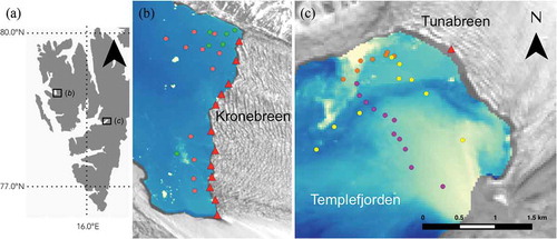
Both Kronebreen and Tunabreen are ideal locations to study sediment plumes because the fjord depths at their termini are relatively shallow (<60 m and about 40 m, respectively; Trusel et al. 2010; Flink et al. 2015). This shallow depth allows minimal time for a subglacially released meltwater plume to entrain enough ambient ocean water to equilibrate before reaching the surface, which has been observed in deep Greenlandic fjords (cf. Straneo et al. 2011; Xu et al. 2013; Chauché et al. 2014), and could be problematic for this study. Additionally, Kronebreen and Tunabreen’s termini are largely mélange- and sea ice-free May–August and have fairly consistent sediment plumes visible at the fjord surface. Previous work looking at submarine melt and calving processes (Luckman et al. 2015) has shown that the behaviour of these two glaciers may be typical of medium-sized glaciers terminating in fjords experiencing a seasonal incursion of warm water. Therefore, we suspect, they may also have typical meltwater discharge behaviour and be representative of many high-latitude Arctic glaciers.

2.2. SSC sampling

We collected surface water samples at 44 sample locations (Figure 1), using four 250 ml water bottles at each of the 17 sampling locations in Kongsfjorden, and two 1000 ml water bottles at each of the 27 sampling locations in Templefjorden. We created duplicate samples for each site by first measuring the volume of each water sample, and then running half of the total water collected through a Suction Buchner filter configuration with a vacuum hand pump (two 250 ml samples from Kongsfjorden and one 1000 ml sample from Templefjorden per filter). Each filter (45 mm diameter, 47 μm cellulose filter) was weighed before and after filtration on a 1.00 × 10⁻³ g precision balance. The SSC was calculated by dividing the mass of sediment (difference in pre- and post-filter weight, mg) by the volume of water (l). The two measurements of SSC for each location were then averaged to get one SSC value at each sample location.

We collected water over 5 days, in two different fjords, at 100 m intervals along transects running parallel and perpendicular to the two tidewater glacier termini (Figure 1). Sampling locations include both inside and outside of plumes, regions free of floating ice, and temporally covering periods of high and low glacier run-off during the 2015 summer melt season. We sampled Kongsfjorden on the mornings of 2 and 4 May (days 222 and 224) and Templefjorden on the afternoons of 10, 13, and 14 of August (days 222, 225, and 226, respectively).

2.3. In situ surface reflectance

At every water-sampling location, we also measured fjord spectral reflectance using an Ocean Optics Jaz spectrometer, with a fibre-optic cable. We calibrated the spectrometer at each site using a LabSphere high-reflectance white Lambertian panel and then made three to four repeated spectral measurements with the tip of the fibre-optic cable suspended pointing downward, approximately 1 cm below the water surface on the sunlit side of the boat. This ensured that the measurements of upwelling spectral radiance were not affected by specular reflection or the boat’s shadow. During processing, we averaged together the reflectance profiles for each location to create one reflectance profile for each sample location. After reviewing the profiles for obvious blunders, we applied the Landsat-8 weighting to the field spectra profiles creating reflectance values in simulated Landsat-8 bands.

2.4. Landsat-8 surface reflectance

To investigate the relationship between measured SSC and plume reflectance in satellite imagery, we used imagery from the Landsat-8 OLI Level-1 surface reflectance product. The surface reflectance product applies a correction to the satellite-derived top of atmosphere reflectance values to remove the scattering and absorbing of atmospheric gases and aerosols, resulting in the reflectance that would be measured at the ground level without the presence of an atmosphere (Vermote et al. 2016). The algorithm used to eliminate atmospheric effects and create the Landsat-8 OLI surface reflectance product uses atmospheric and aerosol data input from the Landsat-8 coastal aerosol band, as well as MODIS and Visible Infrared Imaging Radiometer Suite. The success of the algorithm, in comparison to previous Landsat sensors (Landsat 7/ETM+ and Landsat 5/TM), is enhanced by the Landsat-8 design with narrow bands located at wavelengths that are less subject to atmospheric absorption (Vermote et al. 2016).

To best establish a relationship between measured SSC and plume reflectance, we used Landsat-8 surface reflectance images coinciding to the closest dates of our field measurements; we used images collected on 2 May 2015 and 4 May 2015 (days 122 and 124) for comparison with the corresponding Kongsfjorden field data, and the image collected on 10 August 2015 (day 222) for comparison with all of the Templefjorden data (days 222, 225, and 226). Landsat-8 has a 16 days repeat orbit; however, at the high latitude of these study sites (about 78°N), repeat satellite coverage is between 2 and 4 days. While not as high of temporal resolution as MODIS (previously used by Chu et al. 2009; McGrath et al. 2010; Chu et al. 2012; Tedstone and Arnold 2012; Hudson et al. 2014; Schild, Hawley, and Morriss 2016), we chose to use the Landsat-8 imagery because its higher spatial resolution (30 m compared to MODIS 250 or 500 m) better resolves the smaller glaciers and fjords of our study sites.

2.5. Comparing in situ and satellite sampling methods

To validate the Landsat-8 surface reflectance product, we compare reflectance values at our sampling locations (Figure 2) using the field spectral reflectance data in the simulated Landsat-8 red (640–670 nm) and NIR (850–880 nm) bands. The slope of the best-fit lines between in situ and remotely collected surface reflectance for red is 1.12 (95.0% confidence interval 0.89–1.34) and 1.04 for red + NIR (95.0% confidence interval 0.83–1.25). The y intercept for red is −6.30 (95.0% confidence interval −9.96 to −2.78) and −8.39 for red + NIR (95.0% confidence interval −12.79 to −3.99). This non-zero intercept, in spite of the slope being statistically indistinguishable from one, indicates that in situ surface reflectance and Landsat-8 surface reflectance are not interchangeable. A difference between in situ and Landsat-8 surface reflectance is expected; while the Landsat-8 surface reflectance product removes atmospheric attenuation, these measurements still include radiance from specular reflection off the water surface, whereas the in situ measurements, collected just below the water surface, do not. We attribute the offset between the two measurements primarily to the inclusion of radiance from specular reflection in the Landsat-8 product and not the in situ measurements. We note that even if we had collected in situ measurements just above the water surface, thus including specular reflectance off the water, the Landsat-8 and in situ measurements would still not be comparable because the slopes of the waves and the angle of the sensors would be different, leading to a highly variable specular component.

Figure 2. Comparison between Landsat-8 surface reflectance product and in situ field spectrometer reflectance measurements for the red (red diamonds) and red + NIR (black diamonds) spectral ranges at all 44 sample locations. Measure of scatter between the points and the corresponding coloured best-fit line shows the correlation between Landsat-8 surface reflectance product and in situ measurements (r² value of 0.70).

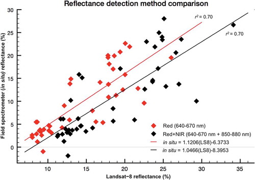
Additionally, we calculated the root mean square error (RMSE) between Landsat-8 and in situ measurements of surface reflectance. We found a RMSE in Landsat-8 red reflectance to be 3.4%, and a RMSE in Landsat-8 red + NIR reflectance to be 8.9%. Although the satellite and in situ reflectance values are generally similar, we chose to separate the reflectance values of these two collection methods in all further analysis due to the offset. For clarity, we distinguish between the field spectrometer reflectance values and the Landsat-8 reflectance values by identifying the collection method and associated colour (e.g. in situ red band, Landsat-8 red + NIR band) even though both reference the wavelength range and weighting of the Landsat-8 sensor.

2.6. Calculating surface sediment load

Previous plume metrics used to study meltwater discharge, namely plume area and plume length (Dowdeswell and Cromack 1991), have a fairly good relationship with meltwater run-off at land-terminating glaciers (Chu et al. 2009; McGrath et al. 2010) but do not display the same relationship at tidewater glaciers (Chu et al. 2012; Tedstone and Arnold 2012). This is likely due to the plume itself being influenced by fjord stratification, circulation, and depth. Therefore, we established and tested an alternative metric, total surface suspended sediment load, to observe relative meltwater discharge throughout the 2015 Kronebreen and Tunabreen melt seasons. This provides insights on meltwater transit time, glacier melt response rates, and fjord residence time.

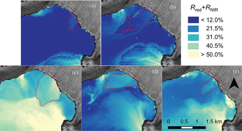
To calculate the total surface sediment load, we first delineate the area of the plume using a reflectance threshold of 12.0% in the red + NIR band for all cloud-and ice-free Landsat-8 imagery of Kongsfjorden and Templefjorden for the 2015 summer melt season (Figure 3, red lines). We were bounded early in the melt season by the presence of winter sea ice at the terminus (Tunabreen) or high solar zenith angles (Kronebreen) and bounded late in the season by high solar zenith angles making the Landsat-8 surface reflectance product unavailable. In instances where the entire fjord has reflectance values greater than 12.0%, we set the plume extent as the minimum reflectance between the subglacial plume, and the terrestrial run-off plumes (e.g. Figure 3(c)–(e), days 213–229). We then calculated the sediment mass for each pixel (mg), by first calculating the SSC of each pixel (mg l⁻¹) based on the Landsat-8 red + NIR reflectance relationship (established in Section 3.1) and then multiplying by the volume of water in that pixel (l). We calculated the volume of surface water by multiplying the pixel area (30 m × 30 m) by a depth of 0.20 m, the height of our bottle used for water sample collection, and therefore the maximum depth of water used to establish the in situ SSC measurement. Lastly, we summed all of the sediment load values inside of the established sediment plume area, arriving at what we refer to as the total surface sediment load (kg).

Figure 3. The five Landsat-8 red + NIR surface reflectance images used from Tunabreen (location map, Figure 1(a)), spanning the summer 2015 melt season, showing the subglacial plume discharge location (red triangle), and subglacial sediment plume boundaries (solid red line). These five images from days 187 (a), 190 (b), 213 (c), 226 (d), and 229 (e) are collected between 3 and 23 days apart and highlight the dynamic nature of sediment plumes.

2.7. Meltwater

In lieu of attempting to quantify meltwater run-off, we use positive degree days (PDDs) as a proxy for meltwater availability at Kronebreen and Tunabreen (Hock 2003; Bartholomew et al. 2010; Chu et al. 2012; Schild and Hamilton 2013). We calculate the daily PDD values using the average daily temperature measurements collected from automatic weather station at Ny-Ålesund (78.92°N, 11.93°E, 8 masl), 15 km west of Kronebreen, and Pyramiden (78.65°N, 16.35°E, 20 masl), 32 km north of Tunabreen. Following the methods of Schild and Hamilton (2013), the daily average temperature after the onset of melt is defined as the PDD value for each day. To take into account lags in the hydraulic system introduced by finite transit time of meltwater through the glacier system and potential subglacial storage, we construct a ‘lag index’ using accumulated PDDs. This index is the cumulative sum of the PDDs in the 6 days prior to that day, or the date of image acquisition.

3. Results

3.1. Surface reflectance and SSC

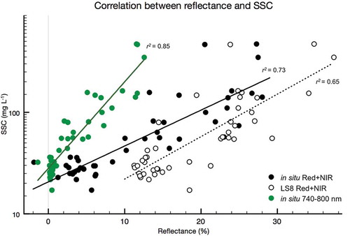
Using the Landsat-8 surface reflectance product, and the 44 in situ measurements of surface reflectance and SSC, we established empirical relationships between Landsat-8 surface reflectance and in situ surface reflectance (red and red + NIR bands) with measured SSCs (Figure 4). The model with the highest correlation related the field spectrometer in the red + NIR range and SSC, with an r² value of 0.73 (Table 1). In all cases, models based on in situ reflectance were better predictors of SSC than were the models based on the Landsat-8 reflectance in the same wavelength range (Table 1).

Table 1. Derived equations relating surface reflectance in red and red + NIR wavelengths to SSC at both tidewater glaciers (TWG) and land-terminating glaciers (LTG) in Svalbard and Greenland.

Row	Collection method	SSC range (mg l^−1)	Number of samples	Glacier type, number	SSC (mg)	r^2
1	Landsat-8	0–450	44	2 TWG		0.56
2	Landsat-8	0–450	44	2 TWG		0.65
3	In situ	0–450	44	2 TWG		0.63
4	In situ	0–450	44	2 TWG		0.73
5	Landsat-8	0–200	41	2 TWG		0.55
6	Landsat-8	0–200	41	2 TWG		0.61
7	In situ	0–200	41	2 TWG		0.69
8	In situ	0–200	41	2 TWG		0.75
9	Chu et al. (2009) In situ	0–500	22	1 LTG		0.90
10	Chu et al. (2012) In situ	0–500	25	1 LTG, 1 TWG		0.85
11	Hudson et al. (2014) MODIS	1.20–716	143	3 LTG		0.84

Columns indicate the sensor used to collect the reflectance measurements, the range of SSC values, the number of samples collected, the number of glacier locations and type of glaciers in each calculation, the reflectance equation, and corresponding r² values (columns 2–7, respectively). Rows 1–8 show relationships established in this study, rows 9–11 show the equations derived in other field and remote-sensing studies. It is important to note that Chu et al. (2009), Chu et al. (2012), and Hudson et al. (2014) used the MODIS-equivalent red and NIR wavelength ranges for their calculations, which differs slightly from the Landsat-8 wavelength ranges for the same colours.

Figure 4. Landsat-8 surface reflectance values (open circles) and in situ field spectrometer reflectance measurements (solid circles) against SSC measurements for all 44 sample locations. The lines represent the best-fit between reflectance and SSC for SSCs in the 0–450 mg l⁻¹ range (all 44 samples) and 0–200 mg l⁻¹ range (41 samples) and for in situ and satellite reflectance sampling methods, in the red band range (left) and red + NIR band range (right). Legends correspond to both plots.

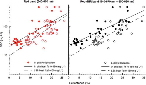
While we were successful in collecting a range of SSC values below 200 mg l⁻¹, there was a gap with no samples between 200 and 300 mg l⁻¹, and only three samples were above 300 mg l⁻¹. To test whether these high SSC values artificially enhanced the r² value, we fit a linear model to a subset of our original data set, including only samples with SSC < 200 mg l⁻¹. While the r² values for all four models are comparable (Table 1), the models limited to the lower range of SSC data have slightly higher r² values than their full data set counterparts, suggesting that in the absence of more robust data at higher SSC values, the models limited to the lower range are preferred.

3.2. Total surface sediment load and meltwater run-off

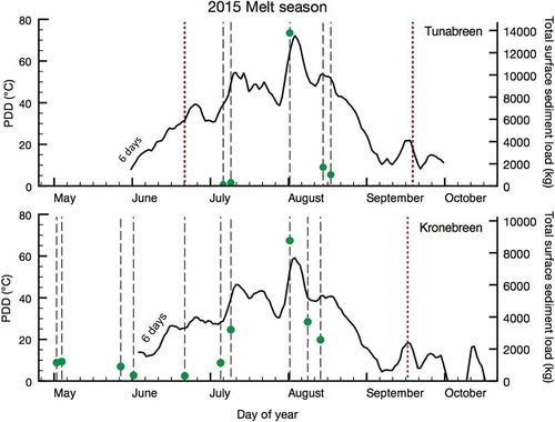
For the 2015 melt season, we were able to use 10 Landsat-8 images at Kronebreen and five images at Tunabreen (Figure 3) to calculate the total surface sediment load (Table 2). The combined 15 images were collected between 2 and 23 days apart, and the variability in plume size, shape, length, and sediment concentration is visible (Figure 3), as well as the subglacial discharge locations (one at Kronebreen, 12 at Tunabreen, Figure 1, red triangles). Of the 10 Kronebreen images, four occurred before the onset of melt and were therefore removed from comparisons between total surface sediment load and accumulated PDDs. We find high correlations between total surface sediment load and accumulated PDDs at both Kronebreen (r² = 0.89, p < 0.005) and Tunabreen (r² = 0.94, p < 0.006, Table 2). Additionally, when considering the temporal distribution of the Landsat-8 images within the melt season (Figure 5, dashed lines), the highest total surface sediment load at both Kronebreen (day 213) and Tunabreen (day 213) coincides with the peak of the melt season.

Table 2. Plume area (m²), calculated surface sediment load (kg), and constructed 6 days PDD value (°C) for each ice- and cloud-free image during the summer 2015 melt season at Kronebreen and Tunabreen glaciers.

DOY	Glacier	Plume area (m^2)	Surface sediment load (kg)	6 days PDD (°C)	r^2 (p-value)
122	Kronebreen	1289,700	1151.60	–	–
124	Kronebreen	1649,700	1216.96	–	–
147	Kronebreen	140,400	904.97	–	–
152	Kronebreen	22,500	354.34	–	–
172	Kronebreen	407,700	318.88	25.40	0.89 (p < 5 × 10^−^3)
186	Kronebreen	1102,500	1134.12	28.30
190	Kronebreen	1394,100	3203.07	39.70
213	Kronebreen	6617,700	8765.42	53.10
220	Kronebreen	3326,400	3695.43	40.00
225	Kronebreen	2628,000	2573.81	40.80
187	Tunabreen	180,000	112.54	39.10	0.94 (p < 6 × 10^−^3)
190	Tunabreen	537,300	290.88	49.50
213	Tunabreen	841,500	13,774.97	64.50
226	Tunabreen	558,900	1682.94	53.60
229	Tunabreen	322,200	1009.50	51.60

The correlation between surface sediment load and constructed 6 days PPD values (r² value) as well as significance (p-value) are shown for Kronebreen and Tunabreen glaciers. Each calculation includes only points with both a surface sediment load value and a constructed 6 days PDD value.

Figure 5. Plot showing the constructed 6 days PDD sum prior to the data point (solid black line) over the 2015 melt season at Tunabreen (top) and Kronebreen (bottom), with the dashed black lines indicating the days of Landsat-8 imagery, and the red dotted lines indicating the start and end of the plume viewing period; the start being the first image with an ice-free terminus and the end being the first image with a solar zenith angle too high to calculate surface reflectance. The total surface sediment load for each of the Landsat-8 images is shown as green dots.

4. Discussion

4.1. Total surface sediment load

While the empirical relationship between SSC and surface reflectance will vary based upon the satellite sensor and band width (e.g. Table 1), sediment plumes remain an indication of meltwater discharge. We argue that using total surface sediment load is a useful metric for estimating meltwater discharge at tidewater glaciers. The spatial variability of plumes, as well as the difference in the relationship between total surface sediment load and constructed PDDs in the two field locations (Figure 5), highlights the importance of fjord geometry, ocean stratification, sediment supply, and plume dynamics in different fjord systems. These factors affect the size, depth, and concentration of a sediment plume and necessitate the development of site-specific relationships, potentially even season-specific relationships, between total surface sediment load and meltwater discharge (variability also noted in McGrath et al. 2010; Tedstone and Arnold 2012; Hudson et al. 2014). While these calculations of total surface sediment load do not give the full sediment load across all depths, nor a direct measurement of meltwater discharge, the change in total surface sediment load could indicate discharge events or periods of time with increased or decreased meltwater run-off for individual drainage basins.

The presence of a plume in the four early season images at Kronebreen likely indicates the presence of over winter subglacial storage as suggested in other glacier systems (Rennermalm et al. 2013; Schild, Hawley, and Morriss 2016). As the melt season progresses, the total surface sediment load follows the calculated 6 days PDD sum with low values early in the melt season, a peak during a large melt period, and then decreases later in the season. At land-terminating glaciers, this late-season sediment decrease has been attributed to the exhaustion of available sediment, not a decrease in meltwater run-off (Schneider and Bronge 1996; Chu et al. 2009; McGrath et al. 2010). However, tidewater glaciers generally have higher velocities than similarly sized land-terminating glaciers and therefore higher bedrock erosion rates, so sediment exhaustion may not be a large concern for end of season at tidewater glaciers.

4.2. Identifying an optimal wavelength range to determine SSCs

In comparing Landsat-8 bands with our field spectrometer profiles, we note a wavelength range (670–850 nm) between the red and NIR bands, presently not covered by the Landsat-8 OLI (Figure 6). To determine an optimal ‘band,’ we divide this wavelength range (670–850 nm) into 10 nm segments and then combine groups of segments to create new ‘bands’ until finding the wavelength range with the highest correlation to SSC. The highest r² value in our study (0.85) occurs with the wavelength range of 740–800 nm (Figure 7). As noted earlier, the r² values for the Landsat-8 reflectance and SSC relationship were all lower than the field spectrometer and SSC relationship (Tables 1 and 2), so we predict that the correlation value for a hypothetical satellite-derived product in this same wavelength range would not be as high as for our field spectrometer but would be higher than the correlations with currently available Landsat-8 spectral bands.

Figure 6. Average spectral profile (purple line) collected in a subglacial plume at Templefjorden. Filled curves represent the Landsat-8 spectral range and weighting function for the blue, green, red, and NIR bands (from left to right), while the dashed line represents the optimal range for SSC detection (740–800 nm), and the bracket indicating the wavelength gap between the red and NIR bands.

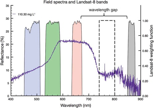
Figure 7. SSC versus surface reflectance in 740–800 nm (green circles, 740–800 nm) plotted along side the models (from Figure 4) with the highest r² value relationships collected from the field spectrometer (red + NIR, black circles) and the Landsat-8 surface reflectance product (red + NIR, open circles). We recommend the spectral range 740–800 nm be considered for inclusion in the next space mission.

To validate this optimal range, we would need satellite imagery over our field location, collected concurrently to our field measurements, in the 740–800 nm wavelength range. Presently, only three operational NASA sensors include part of this range, MODIS band 15 (743–753 nm, 1000 m), Earth Observing 1 (EO-1) Advanced Land Imager (ALI) band 4 (775–805 nm, 30 m), and EO-1 Hyperion bands 39–44 (742.20–793.13 nm, 30 m). Unfortunately, the imagery from these sensors is either not of high enough spatial resolution to resolve SSC changes in smaller fjords (MODIS band 15), was not tasked to cover the field locations during sampling (EO-1 ALI band 4), or the orbital inclination was too low to cover Svalbard and was not operational during sampling (EO-1 Hyperion). Additionally, the EO-1 satellite is scheduled to be decommissioned at the end of the 2016 calendar year, making any efforts for simultaneous EO-1 satellite and ground measurements after this time impossible. Validating the use of this intermediate spectral range for remote estimation of SSC in plumes discharged from tidewater glaciers could be a task for future airborne hyperspectral missions.

5. Conclusions

Tidewater glaciers account for only 35.0% of glaciers worldwide but are contributing about 76.5% to global sea level rise (Gardner et al. 2013). Presently, about half of the mass loss contributing to sea level rise is through the discharge of icebergs, and half through submarine melting and meltwater run-off (van den Broeke et al. 2009; Rignot et al. 2011). However, these tidewater glacier regions are challenging to study in situ; therefore, we need to establish a method to quantify and monitor discharge at these difficult to access glaciers. We used high-resolution (30 m) remote sensing to establish empirical relationships among the Landsat-8 OLI surface reflectance product, in situ field surface reflectance, and in situ measurements of SSC. We found that for the red and red + NIR spectral ranges, r² values were higher when comparing in situ field surface reflectance with SSC than satellite-derived surface reflectance with SSC. This difference in reflectance values based on the collection method demonstrates empirical relationships cannot be used interchangeably.

We used the in situ field spectrometer measurements and SSCs to establish an optimal spectral range (740–800 nm) for observing changes in SSC at tidewater glaciers. Presently, most moderate- or high-resolution satellite systems do not cover this range with high enough spatial resolution or image availability to resolve smaller fjords (<3 km). We recommend that this spectral range be included on future terrestrial Earth-observing satellite missions to support future research on these difficult but important tidewater glacier locations.

Additionally, we used the Landsat-8 red + NIR and SSC relationship (Figure 4, right; Table 1) to identify the total surface sediment load of subglacial sediment plumes across 15 images covering the 2015 melt seasons at Tunabreen and Kronebreen, and found a high correlation (r² ≥ 0.89) between total surface sediment load and meltwater availability (using PDDs) at tidewater glaciers (Figure 5). This strong correlation suggests that we can use total surface sediment load as a measurement of relative meltwater run-off at tidewater glaciers. While this preliminary method does not result in absolute discharge quantities, it enables analysis of relative changes in meltwater run-off at tidewater glaciers with surface expressions of sediment plumes.

Acknowledgements

We would like to thank the NSF IGERT and the NSF GK-12 awards (Awards DGE-0801490 and DGE-0947790, respectively) for training grants to fund KMS; the American Alpine Club, The Geological Society of America, the Dartmouth Earth Sciences Department, the ConocoPhillips-Ludin Northern Area Program (under the CRIOS project), and NASA (Award NNX10AG22G) for their financial support to conduct the fieldwork; UNIS and KingsBay for field logistic support. We would also like to thank all those that loaned field equipment: Steve Arcone, Jack Kohler, Xiahong Feng, Erich Osterberg; those that assisted in data collection: Penny How, Katrin Lindbäk, Ankit Pramanik, and Christian Zolley; the scientific editor for this manuscript, Prof. Arthur Cracknell, and the two anonymous referees who provided helpful and insightful suggestions.

Disclosure statement

No potential conflict of interest was reported by the authors.

Additional information

Funding

This work was supported by National Science Foundation IGERT award: [Grant Number DGE-0801490]; National Science Foundation GK-12 award: [Grant Number DGE-0947790]; NASA supplement award: [Grant Number NNX10AG22G]; American Alpine Club under their Research Grant; Geological Society of America under their Research Grant; the ConocoPhillips-Ludin Northern Area Program under the CRIOS project (Calving Rates and Impact on Sea Level); and Dartmouth Earth Sciences Department.

References

- Baker, E. T., and J. W. Lavelle. 1984. “The Effect of Particle-Size on the Light Attenuation Coefficient of Natural Suspensions.” Journal of Geophysical Research-Oceans 89 (Nc5): 8197–8203. doi:10.1029/Jc089ic05p08197.
- Bartholomew, I., P. Nienow, D. Mair, A. Hubbard, M. A. King, and A. Sole. 2010. “Seasonal Evolution of Subglacial Drainage and Acceleration in a Greenland Outlet Glacier.” Nature Geoscience 3 (6): 408–411. doi:10.1038/ngeo863.
- Binding, C. E., D. G. Bowers, and E. G. Mitchelson-Jacob. 2005. “Estimating Suspended Sediment Concentrations from Ocean Colour Measurements in Moderately Turbid Waters; the Impact of Variable Particle Scattering Properties.” Remote Sensing of Environment 94 (3): 373–383. doi:10.1016/j.rse.2004.11.002.
- Chauché, N., A. Hubbard, J. C. Gascard, J. E. Box, R. Bates, M. Koppes, A. Sole, P. Christoffersen, and H. Patton. 2014. “Ice-Ocean Interaction and Calving Front Morphology at Two West Greenland Tidewater Outlet Glaciers.” The Cryosphere 8 (4): 1457–1468. doi:10.5194/tc-8-1457-2014.
- Chu, V. W., L. C. Smith, A. K. Rennermalm, R. R. Forster, and J. E. Box. 2012. “Hydrologic Controls on Coastal Suspended Sediment Plumes around the Greenland Ice Sheet.” The Cryosphere 6 (1): 1–19. doi:10.5194/tc-6-1-2012.
- Chu, V. W., L. C. Smith, A. K. Rennermalm, R. R. Forster, J. E. Box, and N. Reeh. 2009. “Sediment Plume Response to Surface Melting and Supraglacial Lake Drainages on the Greenland Ice Sheet.” Journal of Glaciology 55 (194): 1072–1082. doi:10.3189/002214309790794904.
- Church, J. A., and N. J. White. 2006. “A 20th Century Acceleration in Global Sea-Level Rise.” Geophysical Research Letters 33 (L01602): 4. doi:10.1029/2005GL024826.
- Dowdeswell, J. A., and M. Cromack. 1991. “Behavior of a Glacier-Derived Suspended Sediment Plume in a Small Arctic Inlet.” Journal of Geology 99 (1): 111–123. doi:10.1086/629477.
- Doxaran, D., J. M. Froidefond, S. Lavender, and P. Castaing. 2002. “Spectral Signature of Highly Turbid Waters - Application with SPOT Data to Quantify Suspended Particulate Matter Concentrations.” Remote Sensing of Environment 81 (1): 149–161. doi:10.1016/S0034-4257(01)00341-8.
- Enderlin, E. M., I. M. Howat, S. Jeong, M. J. Noh, J. H. van Angelen, and M. R. van den broeke. 2014. “An Improved Mass Budget for the Greenland Ice Sheet.” Geophysical Research Letters 41 (3): 866–872. doi:10.1002/2013gl059010.
- Flink, A. M., R. Noormets, N. Kirchner, D. I. Benn, A. Luckman, and H. Lovell. 2015. “The Evolution of a Submarine Landform Record following Recent and Multiple Surges of Tunabreen Glacier, Svalbard.” Quaternary Science Reviews 108: 37–50. doi:10.1016/j.quascirev.2014.11.006.
- Gardner, A. S., G. Moholdt, J. G. Cogley, B. Wouters, A. A. Arendt, J. Wahr, E. Berthier, et al. 2013. “A Reconciled Estimate of Glacier Contributions to Sea Level Rise: 2003 to 2009.” Science 340 (6134): 852–857. doi:10.1126/science.1234532.
- Gurnell, A. M., and J. Warburton. 1990. “The Significance of Suspended Sediment Pulses for Estimating Suspended Sediment Load and Identifying Suspended Sediment Sources in Alpine Glacier Basins.” Hydrology of Mountainous Regions 1: 463–470.
- Hagen, J. O., K. Melvold, F. Pinglot, and J. A. Dowdeswell. 2003. “On the Net Mass Balance of the Glaciers and Ice Caps in Svalbard, Norwegian Arctic.” Arctic Antarctic and Alpine Research 35 (2): 264–270. doi:10.1657/1523-0430(2003)035[0264:OTNMBO]2.0.CO;2.
- Hallet, B., L. Hunter, and J. Bogen. 1996. “Rates of Erosion and Sediment Evacuation by Glaciers: A Review of Field Data and Their Implications.” Global and Planetary Change 12 (1–4): 213–235. doi:10.1016/0921-8181(95)00021-6.
- Hock, R. 2003. “Temperature Index Melt Modelling in Mountain Areas.” Journal of Hydrology 282 (1–4): 104–115. doi:10.1016/s0022-1694(03)00257-9.
- Howat, I. M., Y. Ahn, I. Joughin, M. R. van den Broeke, J. T. M. Lenaerts, and B. Smith. 2011. “Mass Balance of Greenland’s Three Largest Outlet Glaciers, 2000-2010.” Geophysical Research Letters 38. doi:10.1029/2011gl047565.
- Hubbard, B., and P. Nienow. 1997. “Alpine Subglacial Hydrology.” Quaternary Science Reviews 16 (9): 939–955. doi:10.1016/S0277-3791(97)00031-0.
- Hudson, B., I. Overeem, D. McGrath, J. P. M. Syvitski, A. Mikkelsen, and B. Hasholt. 2014. “MODIS Observed Increase in Duration and Spatial Extent of Sediment Plumes in Greenland Fjords.” The Cryosphere 8: 1161–1176. doi:10.5194/tc-8-1161-2014.
- Jacob, T., J. Wahr, W. T. Pfeffer, and S. Swenson. 2012. “Recent Contributions of Glaciers and Ice Caps to Sea Level Rise.” Nature 482 (7386): 514–518. doi:10.1038/nature10847.
- Kääb, A. 2008. “Glacier Volume Changes Using ASTER Satellite Stereo and ICESat GLAS Laser Altimetry. A Test Study on Edgeoya, Eastern Svalbard.” IEEE Transactions on Geoscience and Remote Sensing 46 (10): 2823–2830. doi:10.1109/tgrs.2008.2000627.
- Kohler, J., T. D. James, T. Murray, C. Nuth, O. Brandt, N. E. Barrand, H. F. Aas, and A. Luckman. 2007. “Acceleration in Thinning Rate on Western Svalbard Glaciers.” Geophysical Research Letters 34 (18): 5. doi:10.1029/2007GL030681.
- König, M., C. Nuth, J. Kohler, G. Moholdt, and R. Pettersson. 2013. “A Digital Glacier Database for Svalbard.” In Global Land Ice Measurements from Space, edited by J. S. Kargel, G. J. Leonard, M. P. Bishop, A. Kaab, and B. H. Raup, 229–239. Berlin: Praxis-Springer.
- Liestøl, O. 1988. “The Glaciers in the Kongsfjorden Area, Spitsbergen.” Norsk Geografisk Tidsskrift - Norwegian Journal of Geography 42 (4): 231–238. doi:10.1080/00291958808552205.
- Luckman, A., D. I. Benn, F. Cottier, S. L. Bevan, F. Nilsen, and M. E. Inall. 2015. “Calving Rates at Tidewater Glaciers Vary Strongly with Ocean Temperature.” Nature Communications 6: 8566–8572. doi:10.1038/ncomms9566.
- McGrath, D., K. Steffen, I. Overeem, S. H. Mernild, B. Hasholt, and M. van den Broeke. 2010. “Sediment Plumes as a Proxy for Local Ice-Sheet Runoff in Kangerlussuaq Fjord, West Greenland.” Journal of Glaciology 56 (199): 813–821. doi:10.3189/002214310794457227.
- Miller, R. L., and B. A. McKee. 2004. “Using MODIS Terra 250 M Imagery to Map Concentrations of Total Suspended Matter in Coastal Waters.” Remote Sensing of Environment 93 (1–2): 259–266. doi:10.1016/j.rse.2004.07.012.
- Nuth, C., J. Kohler, H. F. Aas, O. Brandt, and J. O. Hagen. 2007. “Glacier Geometry and Elevation Changes on Svalbard (1936-90): A Baseline Dataset.” Annals of Glaciology 46 (1): 106–116. doi:10.3189/172756407782871440.
- Rennermalm, A. K., L. C. Smith, V. W. Chu, J. E. Box, R. R. Forster, M. R. van den Broeke, D. Van As, and S. E. Moustafa. 2013. “Evidence of Meltwater Retention within the Greenland Ice Sheet.” The Cryosphere 7 (5): 1433–1445. doi:10.5194/tc-7-1433-2013.
- Rignot, E., I. Velicogna, M. R. van den Broeke, A. Monaghan, and J. T. M. Lenaerts. 2011. “Acceleration of the Contribution of the Greenland and Antarctic Ice Sheets to Sea Level Rise.” Geophysical Research Letters 38 (5): 5. doi:10.1029/2011gl046583.
- Schild, K. M., and G. S. Hamilton. 2013. “Seasonal Variations of Outlet Glacier Terminus Position in Greenland.” Journal of Glaciology 59 (216): 759–770. doi:10.3189/2013JoG12J238.
- Schild, K. M., R. L. Hawley, and B. F. Morriss. 2016. “Subglacial Hydrology at Rink Isbræ, West Greenland Inferred from Sediment Plume Appearance.” Annals of Glaciology 57 (72): 118–127. doi:10.1017/aog.2016.1.
- Schneider, T., and C. Bronge. 1996. “Suspended Sediment Transport in the Storglaciaren Drainage Basin.” Geografiska Annaler Series a-Physical Geography 78A (2–3): 155–161. doi:10.2307/520977.
- Shepherd, A., E. R. Ivins, A. Geruo, V. R. Barletta, M. J. Bentley, S. Bettadpur, K. H. Briggs, et al. 2012. “A Reconciled Estimate of Ice-Sheet Mass Balance.” Science 338 (6111): 1183–1189. doi:10.1126/Science.1228102.
- Straneo, F., R. G. Curry, D. A. Sutherland, G. S. Hamilton, C. Cenedese, K. Vage, and L. A. Stearns. 2011. “Impact of Fjord Dynamics and Glacial Runoff on the Circulation near Helheim Glacier.” Nature Geoscience 4 (5): 322–327. doi:10.1038/ngeo1109.
- Straneo, F., P. Heimbach, O. Sergienko, G. Hamilton, G. Catania, S. Griffies, R. Hallberg, et al. 2013. “Challenges to Understanding the Dynamic Response of Greenland’s Marine Terminating Glaciers to Oceanic and Atmospheric Forcing.” Bulletin of the American Meteorological Society 94 (8): 1131–1144. doi:10.1175/bams-d-12-00100.1.
- Tedstone, A. J., and N. S. Arnold. 2012. “Automated Remote Sensing of Sediment Plumes for Identification of Runoff from the Greenland Ice Sheet.” Journal of Glaciology 58 (210): 699–712. doi:10.3189/2012JoG11J204.
- Trusel, L. D., R. D. Powell, R. M. Cumpston, and J. Brigham-Grette. 2010. “Modern Glaciomarine Processes and Potential Future Behaviour of Kronebreen and Kongsvegen Polythermal Tidewater Glaciers, Kongsfjorden, Svalbard.” In Fjord Systems and Archives, edited by J. A. Howe, W. E. N. Austin, M. Forwick, and M. Paetzel. London: Geological Society.
- van de Hulst, H. C. 1957. Light Scattering by Small Particles. New York: Wiley.
- van den Broeke, M., J. Bamber, J. Ettema, E. Rignot, E. Schrama, W. J. van de Berg, E. van Meijgaard, I. Velicogna, and B. Wouters. 2009. “Partitioning Recent Greenland Mass Loss.” Science 326 (5955): 984–986. doi:10.1126/science.1178176.
- Vaughan, D. G., J. C. Comiso, I. Allison, J. Carrasco, G. Kaser, R. Kwok, P. Mote, et al. 2013. “Observations: Cryosphere.” Climate Change 2103: 317–382.
- Vermote, E., C. Justice, M. Claverie, and B. Franch. 2016. “Preliminary Analysis of the Performance of the Landsat 8/OLI Land Surface Reflectance Product.” Remote Sensing of Environment 185: 46–56. doi:10.1016/j.rse.2016.04.008.
- Xu, Y., E. Rignot, I. Fenty, D. Menemenlis, and M. M. Flexas. 2013. “Subaqueous Melting of Store Glacier, West Greenland from Three-Dimensional, High-Resolution Numerical Modeling and Ocean Observations.” Geophysical Research Letters 40 (17): 4648–4653. doi:10.1002/Grl.50825.