Synthetic retrieval of hourly net ecosystem exchange using the neural network model with combined MI and GOCI geostationary sensor datasets and ground-based measurements

ABSTRACT

Net ecosystem carbon dioxide (CO₂) exchange (NEE) is a key parameter for understanding the terrestrial plant ecosystems, but it is difficult to monitor or predict over large areas at fine temporal resolutions. In this research, we estimated the hourly NEE using a combination of the integrated neural network (NN) model with geostationary satellite imagery to overcome the limitations of existing daily polar orbiting satellite-derived carbon flux products. Two sets of satellite imageries (i.e. the meteorological imager (MI) and geostationary ocean colour imager (GOCI) aboard communication, ocean, and meteorological satellite (COMS)) and CO₂ flux data derived from eddy covariance measurements were used to verify the feasibility of applying hourly geostationary satellite imagery with an NN-based approach for estimating NEE at high temporal resolutions. For the NN model, the optimum neuronal architecture was established using an NN with one hidden layer that was trained using the Levenberg–Marquardt back propagation algorithm. The hourly NEE values estimated in test period from the NN model using the combined COMS MI and GOCI imagery and ground measurements as model inputs were compared with the eddy covariance NEE values from the measurement tower, which yielded reliable statistical agreement. The hourly NEE results from the NN model based on COMS MI and GOCI imagery and ground measurement data had the highest accuracy (RMSE = 2.026 μmol m⁻² s⁻², R = 0.975), while the root mean square error (RMSE) and the regression coefficient (R) generated by the NN model based on satellite imagery as the sole input variable were relatively lower (RMSE = 3.230 μmol m⁻² s⁻², R = 0.952). Although the simulations for the satellite-only NEE were showed as lower accuracy than the NN model that included all input variables, the hourly variations in NEE also appeared to describe its daily growth and development pattern well, indicating the possibility of deriving hourly-based products from the proposed NN model using geostationary satellite data as inputs.

1. Introduction

Net ecosystem carbon dioxide (CO₂) exchange (NEE) is considered a key element of the terrestrial biosphere that affects climate system dynamics by controlling land–atmosphere CO₂ fluxes (Canadell et al. 2007; Shim et al. 2014). Traditionally, tower-based eddy covariance measurements have been applied to estimate changes in NEE (Baldocchi et al. 2001; Baldocchi 2003). However, tower-based observations of surface–atmosphere CO₂ exchange can present major challenges (Baldocchi et al. 2001). For instance, it may be difficult to accurately estimate CO₂ fluxes between the terrestrial surface and atmosphere without first understanding complicated micrometeorological interactions. It should be noted that estimating NEE from eddy covariance (NEE_EC) relies on a number of assumptions (e.g. flat, homogeneous terrain and well-mixed atmospheric conditions). The eddy covariance method is most applicable over flat terrain, where the environmental conditions are steady, and the underlying vegetation extends upwind for an extended distance (Baldocchi 2003). If these requirements are violated, the eddy covariance method for estimating NEE can result in significant systematic errors (Baldocchi, Hincks, and Meyers 1988; Foken and Wichura 1996; Massman and Lee 2002). The uncertainties associated with NEE are expected to further increase when the values are integrated over time to produce daily and annual fluctuations (Moncrieff, Malhi, and Leuning 1996). From the perspective of providing information on potential changes in NEE over spatial areas (e.g. agricultural farms or other regions where an understanding of CO₂ exchange is necessary), tower-based NEE measurements have additional inherent limitations. For example, it may be impractical to acquire NEE using the measurement-based approach over large regions where it is difficult to set up the measurement apparatus (Göckede et al. 2008), and alternative methods for estimating NEE over such regions must be explored.

As an alternative to tower-based NEE estimations, a number of studies have applied satellite-based methods to estimate atmospheric carbon cycles (Shim et al. 2014; Tang et al. 2012). Most of these studies have adopted polar-orbiting Moderate Resolution Imaging Spectroradiometer (MODIS) sensors with eddy variance data to spatially estimate carbon flux values, offering, for example, reasonably accurate estimations of net primary productivity and gross primary productivity (GPP) (Justice et al. 2002; Shim et al. 2014). MODIS GPP data span a total of 36 spectral bands, providing very good spatial coverage. However, carbon flux products estimated from MODIS are typically either acquired at daily temporal resolutions or interpolated from a representative daytime value, as MODIS aboard the Terra and Aqua satellites only records observations twice a day in mid-latitude regions. Furthermore, although Wallner (2015) used the geostationary Meteosat Second Generation’s Spinning Enhanced Visible and Infrared Imager (MSG SEVIRI) satellites to calculate GPP, the temporal resolution of the GPP was over a daily time horizon because their algorithm was based on MODIS GPP product methods. Notwithstanding this necessity, modelling the diurnal cycle of NEE values over a vegetation area can provide crucial information for detailed interpretation of the carbon flux exchange between the atmosphere and terrestrial ecosystems.

The technical purpose of this study was to validate the feasibility of obtaining high temporal resolution NEE estimations in a synthetic manner using a neural network (NN) approach in combination with hourly geostationary satellite radiometer data and ground NEE measurements over a selected mixed forest area. It is technically meaningful to estimate hourly NEE products using NN modelling, as such work has yet to be performed in this study region. In terms of the NEE estimation algorithm, the NN method has proved more effective than traditional statistical techniques (e.g. linear regression models) for its ability to incorporate remote-sensing data (Kaminsky, Barad, and Brown 1997; Şahin, Kaya, and Uyar 2013; Yeom and Han 2010). In general, NN models are useful for predictions in areas with nonlinear system modelling and control (Chen and Billings 1992; Wu, Chau, and Li 2009) because they can extract patterns and data attributes from input variables related to changes in the objective variable. In terms of the input data necessary to yield a high temporal resolution, two distinctive geostationary sensors onboard the Communication, Ocean and Meteorological Satellite (COMS) (i.e. meteorological imager (MI) and geostationary ocean colour imager (GOCI)) were used to monitor the carbon flux activity of vegetation over a 24-h period using spectral bands sensitive to the status of vegetation growth and the meteorological environment of the canopy layer. The combined geostationary satellite data provide hourly reflectance and brightness temperature data, offering a greater potential to provide input data to simulate high temporal resolution NEE values compared to polar-orbiting satellites (e.g. MODIS) (Tang et al. 2012).

This study has evaluated the feasibility of using hourly geostationary satellite imagery based on NN modelling to estimate high temporal resolution NEE on Jeju Island, South Korea. This study had three purposes: (1) to apply MI and GOCI geostationary multi-purpose satellite input data to simulate NEE using an NN model trained with the Levenberg–Marquardt backpropagation (LM-BP) algorithm; (2) to validate the model simulations with tower-based flux measurements in an experimental forest on Jeju Island, South Korea; and (3) to evaluate the NN model performance using key statistical metrics by comparing the NEE estimated from combined satellite imagery with ground measurements during both daytime and night-time.

2. Materials and methods

2.1. Satellite data

The data derived from the MI and GOCI sensors onboard the COMS, Korea’s first geostationary multi-purpose satellite, were used as key input values for the NN model simulations to estimate NEE. Table 1 provides detailed information on the GOCI and MI sensors. GOCI includes eight solar spectral bands that perform observations approximately eight times during the daytime (9 a.m. to 4 p.m.). Meanwhile, MI is equipped with visible and infrared (IR) channels; all channels can be used during the daytime (sunrise to sunset), but only the IR channel can be used at night. For complex NEE estimations during the daytime, when active vegetation growth occurs due to photosynthesis, it is important to use as much satellite observation information as possible. In particular, it is important to make maximum use of solar channels, especially the GOCI channels, because solar spectral channels can indirectly observe vegetation growth characteristics. Therefore, in this study, we separated the daytime (light dependent) and night-time (light independent) information based on the criterion of whether the GOCI satellite could make observations. The daytime was defined as 9 a.m. to 4 p.m., during which time both the MI satellite data and the GOCI optical channels could be fully used, and the remainder of the time was defined as night-time. In reality, daytime includes the time from 5 p.m. until sunset, as well as sunrise until 8 a.m.; however, according to the definition used in this study, the former period was incorrectly defined as night-time. Therefore, for the daytime period not included in the GOCI observation time, NEE was calculated using only the MI visible channel and IR channels. We assumed that these calculations based on limited MI satellite data could provide reasonable NEE estimations, as photosynthesis activity around sunrise and sunset is relatively lower than that at noon.

Table 1. Detailed characteristics of the COMS MI and GOCI sensors, which collected the data used as input variables for the NN model.

Satellite sensor (Orbit type)	Wavelength (nm)	Spatial resolution
MI	Visible: 550–800 shortwave infrared: 3500–4000 Water vapor: 6500–7000 Infrared 1: 10,300–11,300 Infrared 2: 11,500–15,500	1000 m (4000 m) at nadir visible (infrared)
GOCI	Band1 402–422 Band2 433–453 Band3 480–500 Band4 545–565 Band5 650–670 Band6 675–685 Band7 735–755 Band8 845–885	500 m in the South Korea region

2.2. Study area and flux measurements

Eddy covariance measurement data were adopted for the NN model because they are the most suitable for NEE estimations, with high temporal resolution and low uncertainty. The flux measurement tower is located in the Jeju Experimental Forest on Jeju Island, South Korea (33°19ʹ5.04ʺN, 126°34ʹ5.01ʺE; see yellow rectangle in Figure 1). In this study area, the average tree height was about 13.70 m and the vegetation type is dominated by mixed forest vegetation of Carpinus tschonoskii, Quercus serrata, Pinus densiflora, and Sasa quelpaertensis, according to the National Institute of Forest Science of Korea. The study area experiences a moderate marine climate, with an annual mean temperature of about 16.20°C, annual precipitation of about 1,850.80 mm, and humidity of 70.70%.

Figure 1. Location of the CO₂ flux tower site (marked with white rectangle) for the eddy covariance measurements on Mt. Halla, Jeju Island, South Korea (Image source from Daum map service through QGIS).

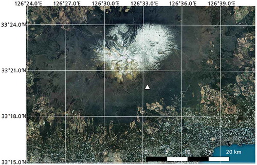
The eddy covariance system consisting of a three-dimensional sonic anemometer and open-path CO₂/H₂O gas analyzer (EC155, Campbell Scientific, USA) and net radiometer (CNR4, Kipp&Zonne, The Netherlands) were installed at a height of 27.00 m and 24.00 m on the flux measurement tower, respectively. These fast-response instruments were operated at a sampling rate of 20 Hz, and the raw data were processed in 30-min intervals. The wind component coordinates were rotated and the density fluctuation correction method was applied to the sonic temperature with the outlier detection and gap filling method (McMillen 1988; Webb, Pearman, and Leuning 1980; Hong et al. 2008; Hong et al. 2009; Hong and Kim 2011). The study period (LTC) during which time hourly CO₂ flux measurements were acquired using the eddy covariance method was selected as 9 May to 19 June 2014.

Parameters related to land surface energy exchange are highly associated with NEE because surface vegetation affects both processes. Thus, the respective temporal data (i.e. month, day, and time) from the ground measurements (i.e. sensible heat flux (W m⁻²), latent heat flux (W m⁻²), net radiation (W m⁻²), and Bowen ratio (ratio of sensible heat to latent heat)) at the flux tower were used as input variables in the NN model, because they provided a broad range of predictive features for the NEE estimation.

2.3. NN model development

To develop a predictive model for NEE from neural network (NEE_NN), two input data sets were designed to separately simulate daytime (light dependent) and night-time (light independent) NEE using the same NN model structure as described in Section 2.1. For the daytime estimations of NEE, we employed the combined MI and GOCI data. For the night-time estimations, only the IR channels of MI were available as inputs for the NN model. In addition, although night-time was defined as the time from 5 p.m. until 8 a.m. due to a lack of GOCI data, it was possible to calculate the NEE from 5 p.m. until sunset and sunrise until 8 a.m. using the MI visible channel and IR channels, because photosynthesis activity in the late afternoon or early morning is lower than that at noon.

In this study, a multilayer feedforward NN with LM-BP algorithm was used to model NEE. LM-BP, which is a second-order nonlinear optimization technique, is usually faster and more reliable than other BP variants (Bertsekas and Tsitsiklis 1996; Masters 1995) and is used to overcome the drawbacks of conventional BP, including slowness and local convergence. In addition, the LM-BP training algorithm is a popular algorithm that provides a numerical solution to the estimation problem by minimizing the sum of the nonlinear least square errors between the observed and predicted outputs in an iterative manner (Levenberg 1944; Marquardt 1963). Since there is no definite and explicit method for selecting the optimal parameters for the prescribed model, a primary issue in training the NN model was to obtain a set of optimally generalized NN for the new training sequence, which applied the defined network to test the validation data in the training set. In this study, we considered different model architectures with iteratively varying hidden neurons. To determine the appropriate number of hidden nodes in the model’s hidden layer, a trial and error method was adopted by changing the number of hidden layer nodes from 1 to 30 in increments of 1. After iteratively tuning the neuronal structure, an early stopping approach (STA) was incorporated with LM-BP to avoid overfitting the NN training and enhance the generalizability of the model (Coulibaly, Anctil, and Bobée 2000).

In our study, we separated the entire data set into three mutually exclusive subsets (training (50%), validation (25%), and testing (25%) sets) and adopted the holdout cross-validation approach. In other words, at least half of the data set was used to train the NN model and determine the most suitable network weights and biases. Next, a suitable model validation data set was established comprising about one-quarter of the entire input data to evaluate the network performance and determine the stop time of the training phase. Once the error of the validation data set started to increase, the NN training was stopped to protect the NN network from overfitting the model input data. Estimating the generalization error by cross-validation with a holdout set allowed us to compare the solutions to determine the stopping phase when the validation error was effectively at a minimum (Coulibaly, Anctil, and Bobée 2000). Finally, the testing set that employed the remainder of the available input data was used to test the effectiveness of the early stopping criterion and evaluate the NN model based on a data set not used in either the training or the validation phase (Prechelt 1998). We separated the matchup data set into three parts based on times within the whole study period to show the hourly variation in the NN-based NEE within the test data set. The test data set period was from 4:00 p.m. 16 May to 10:00 a.m. 23 May (LTC), and remaining data from the study period were used for the training and validation data sets.

Although the holdout cross-validation approach used in this study offers substantial advantages in terms of its efficiency and simplicity, and the proportion of the partitioned data subsets were not strictly restricted (compared to methods that restrict the subsets), it should be acknowledged that improper data splitting can affect the quality of the final predictive model. Therefore, follow-up studies should consider other data splitting approaches such as K-fold cross-validation and leave-one-out cross-validation, as well as statistical techniques such as random sampling, trial and error, purposeful sampling, and convenience sampling, which offer their own merits and constraints (Bowden, Maier, and Dandy 2002; 2005; Reitermanova 2010; Zhang and Berardi 2001).

3. Results

3.1. Sensitivity of the input variables for the NN model

To establish a versatile predictive model for NEE estimation, we performed a sensitivity test by inputting different combinations of variables from the satellite imagery and ground measurement data to determine the optimal input variables for the NN model. The sensitivity test was divided into separate daytime (Figure 2) and night-time (Figure 3) tests based on the time of the GOCI observations.

Figure 2. Scatter plots of net ecosystem carbon dioxide (CO₂) exchange (NEE) derived from eddy covariance measurements compared with the results of the neural network (NN) model estimations based on combined satellite imagery with ground measurements during daytime. (a) Bowen ratio, (b) net solar radiation, Rn, (c) Bowen Ratio and Rn, (d) Meteorological Imager, MI channel, (e) Geostationary Ocean Color Imager, GOCI, (f) MI and GOCI, (g) MI, GOCI, Bowen Ratio, and Rn, (h) MI, GOCI, Sensible heat and Latent and Rn. The black line is the reference line. Bowen, Rn, Sensible, and Latent represent the Bowen ratio, net radiation, sensible heat, and latent heat flux, respectively.

Figure 3. Scatter plots of net ecosystem carbon dioxide (CO₂) exchange (NEE) derived from eddy covariance measurements compared with the results of the neural network (NN) model estimations based on combined satellite imagery with ground measurements during night-time. (a) Bowen ratio, (b) net solar radiation, Rn, (c) Bowen Ratio and Rn, (d) Meteorological Imager, MI channel, (e) Geostationary Ocean Color Imager, GOCI, (f) MI and GOCI, (g) MI, GOCI, Bowen Ratio, and Rn, (h) MI, GOCI, Sensible heat and Latent and Rn. The black line is the reference line. Bowen, Rn, Sensible, and Latent represent the Bowen ratio, net radiation, sensible heat, and latent heat flux, respectively.

Figure 2 shows the scatter plots of the NEE estimated using eddy covariance and the NN method using various input variables, such as the time of observation, data from the GOCI and MI channels, and ground measurements (e.g. sensible heat, latent heat, Bowen ratio, and net radiation). Net radiation, sensible heat, latent heat, and the Bowen ratio were somewhat correlated with NEE (Figure 2(a)–(c)) because the terrestrial–atmosphere exchange of CO₂, water, and energy is critically related to plant physiological processes. The highest accuracy was obtained for the model that included all of the input variables (i.e. MI, GOCI, sensible heat, latent heat, and net radiation), where the R = 0.886 and the RMSE = 3.081 μmol m⁻² s⁻² (Figure 2(h)). This shows that the most accurate simulation of NEE can be achieved using a number of input variables, as expected, since the changes in NEE can be mapped more precisely from the data patterns and attributes of these inputs.

Irrespective of these results, examining only the satellite-based NEE simulations with MI and GOCI input data for the prescribed NN model for spatialization (or enhancing the coverage area) (Figure 2(f)) yielded fairly accurate results. Despite its slightly lower correlation coefficient compared to the NN model based on all inputs (Figure 2(h)), the satellite-based NEE estimation exhibited reasonably accurate agreement (RMSE = 3.672 μmol m⁻² s⁻²) with the NEE determined from the eddy covariance measurements (Figure 2(d)–(f)). For example, NEE values less than 0 μmol m⁻² s⁻² in the daytime eddy covariance measurements, caused by larger canopy photosynthesis than canopy and soil respiration, were estimated as less than zero by the NN model.

The results of the simulated NEE values for the night-time period were consistent with the daytime simulations in terms of the NN model performance metrics. The NN model that included all input variables had the highest accuracy (RMSE = 2.078 μmol m⁻² s⁻²) (Figure 3(f)). In addition, the results of the NN model that included only the MI satellite-based data showed reasonable statistical agreement with the measured values (RMSE = 3.208 μmol m⁻² s⁻²) (Figure 3(d)). At night, respiratory activity of the mixed forest is dominant, with positive NEE values. However, in the scatter plots of the night-time analysis (Figure 3), negative NEE (i.e. CO₂ uptake) values unexpectedly occurred due to the discrepancy between the night and daytimes defined by the GOCI satellite and the real local sunset and sunrise times. For example, daytime carbon uptake from 5 p.m. until sunset and from sunrise until 8 a.m. was categorized as occurring during night-time based on the GOCI satellite observations. At night, which includes late afternoon and early morning, respiration by soil microorganisms and plants dominates, and there is minimal photosynthetic activity (Falge et al. 2002). Thus, the main environmental factor controlling night-time NEE is temperature, particularly soil temperature. This may be a relatively simpler relationship than the major factors that drive daytime NEE. However, the correlations between the measured and estimated NEE did not differ substantially between daytime and night-time.

We determined the final structure of the NN model inputs after careful examination of the sensitivity test. The first criterion for the selection was the accuracy of the estimated NEE from model using various input variables. The second criterion for the selection of the optimum model was based on the potential of the NN model for spatialization (i.e. increased coverage) with the most suitable input variables. Therefore, only the satellite imagery-based inputs for model simulations were used to estimate the temporal NEE over selected mixed forest sites where measurements were challenging to undertake.

3.2. Reducing data dimensionality with principal component analysis

Before applying the final NN simulation model with the combined MI and GOCI imagery and ground measurements as input variables, we normalized the input variables, mainly because the anomalously high or low magnitudes of the input values may not reflect their relative importance in determining the simulated outputs (Jang and Viau 2004). The eigenvectors of the principal component analysis (PCA) from the normalized input data were used to determine the variable dimensions and reduce the multicollinearity of the data set. Reducing data dimensionality is useful for efficiently simulating the model and designing the structure of an NN model. In this study, we applied the PCA technique using the normalized MI, GOCI, and ground measurements to determine an orthogonal system with the minimum dimensions ordered by the magnitude of their variance (Green 1978; Yeom and Han 2010). In addition, NN models based on PCAs are useful for mitigating sensitivity and enhancing the NN prediction capabilities (Balas, Koc, and Tur 2010). Thus, we performed the dimensionality reduction with the PCA in two parts: the first part included all input variables and the second part used only the satellite data for the daytime and night-time periods.

Figure 4 plots the eigenvalues and cumulative percentage of eigenvalues according to the principal component number. Figure 4(a,b) shows the results for only the combined satellite MI and GOCI data used for the NEE simulation for the daytime (a) and night-time (b) periods. Figure 4(c,d) shows the results of all of input variables, including ground-based measurements, used for the NEE simulation with the NN model for the daytime (c) and night-time (d) periods.

Figure 4. Plots of the eigenvalues (in closed dots) and cumulative percentage eigenvalues (in opened dots) according to the principal component number for the daytime (left panels) and night-time (right panels) for: (a, b): combined satellites Meteorological Imager (MI) and Geostationary Ocean Color Imager (GOCI) input data, (c, d): All variables including the ground-based measurements. Each vertical dashed line represents the final principal component number that satisfies the cumulative percentage of eigenvalues of at least 99%.

In this study, a cumulative percentage of eigenvalues of about 99% was adopted as the most appropriate criterion for determining the final data dimensions to reduce redundancy and select the most informative principal components for the developed NN model without discarding any important information in the original data set (Yeom and Han 2010).

3.3. Simulating hourly net ecosystem CO₂ exchange with satellite data

A major objective of this research was to test the preciseness of the NN model for its predictive capability of hourly NEE estimations using combined satellite data, particularly from the perspective of overcoming the temporal resolution of existing daily polar-orbiting satellite-derived carbon flux products. Figure 5 shows the diurnal cycle of the NEE estimations from the eddy covariance relative to the NEE estimation from the NN model with satellite and ground measurement data over a period of 8 days (16–23 May).

Figure 5. Temporal variations in NEE based on the NN simulation model from the test data set (16–23 May) using (a) satellite data (MI and GOCI) as the input variables and (b) all inputs including ground measurements. The red dots represent daytime NEE, and the blue dots represent night-time NEE. The seven light grey areas from 5 p.m. until 8 a.m. represent the night-time period.

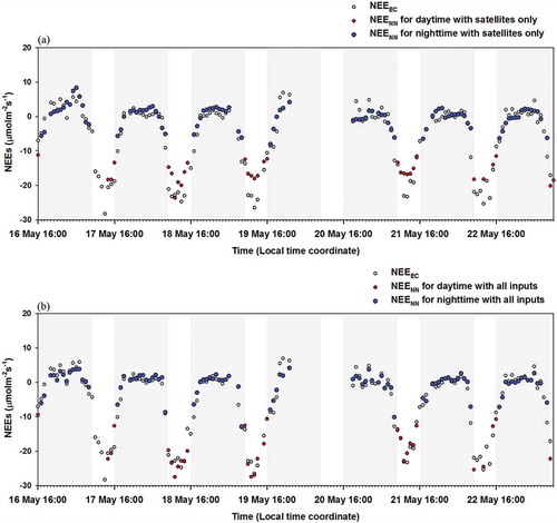
Figure 5(a) shows the results for the satellite only-based NEE simulations, and Figure 5(b) shows the results for all input variables during the daytime and night-time periods. The hourly variations in NEE from the NN model exhibited similar trends to the eddy covariance-based NEE determined from the tower measurements. Overall, including all input variables in the NEE simulation yielded better results (RMSE = 2.026 μmol m⁻² s⁻², R = 0.975) (Figure 5(b)) compared with the NEE values determined from satellite data alone (RMSE = 3.230 μmol m⁻² s⁻², R = 0.952) (Figure 5(a)). When the simulations for the satellite-only NEE were compared, there was significant temporal agreement in the resulting carbon cycles, indicating the possibility of deriving hourly based products and spatialization from the proposed NN model using MI and GOCI data as inputs.

In the case of the daytime period using the satellite data alone as the input variable (Figure 5(a)), the temporal variations in NEE from the eddy covariance measurements matched well, despite some degree of scatter. The scatter was probably due to the difficulty in simulating the complicated carbon flux processes between the fixed forest and atmosphere. In fact, the hourly variations in NEE appeared to describe its daily growth and development pattern well, indicating that the highest carbon intake by plants from the atmosphere occurred around midday, which has the greatest solar energy capacity for vegetation processes. Similarly, around noon, there was a marked decrease in the carbon sink pattern (Figure 5). Some NEE information was missing during the daytime despite simulating the hourly NEE data from satellite information. This was caused by cloud effects, because satellites cannot observe surface properties through clouds using optical sensors.

The hourly NEE profiles from the NN model during the night-time period were more similar to the measured values than were those during the daytime because there was much less plant respiration activity at night. Consistent with the results shown in the scatter plots, most NEE values were located above the zero line, indicative of plant respiration. It should be noted that the NEE patterns were described well from 5 p.m. until sunset and from sunrise until 8 a.m., despite the absence of information from the GOCI visible channel due to the relatively low photosynthesis activity.

4. Discussion

The present study has validated the feasibility of synthetically deriving high temporal resolution NEE estimations using an NN approach in which hourly geostationary satellite data and ground measurements over a selected mixed forest area were validated, and it showed statistically significant results. NN-based model training is often performed with the intent of obtaining a network with optical generalization performance to yield an output when given inputs that were not included in the training set (Coulibaly, Anctil, and Bobée 2000). In this study, we applied holdout cross-validation (i.e. a single data set split into training, validation, and testing sets) rather than k-fold cross-validation. K-fold cross-validation is another robust method that has been suggested to enhance the generalizability of NN modelling. For example, Cutler et al. (2007) performed an integrated fivefold cross-validation process to assess the accuracy, stability, and reliability and generalization ability of the model. In addition, Zhu et al. (2015) showed that BP NN modelling with k-fold cross-validation yielded accurate estimations of unevenly aged and dense mangrove forest biomass.

In this study, we have adopted the LM-BP with STA for the generalization performance of an NN model. Based on previous studies (Coulibaly, Anctil, and Bobée 2000; Jang and Viau 2004; Lauer and Bloch 2006; Prechelt 1998), STA has showed reasonable results to enhance generalization by reducing overfitting. It is difficult to determine the most efficient methods for the generalization of NN simulations; therefore, the question of how effective the abovementioned approaches are for the generalization of other NN algorithms, other error functions, and other data products remains unanswered. It was beyond the scope of this research to address these questions; however, they should be investigated in future work.

Although this study demonstrated the potential for integrating NN models with geostationary satellite data over spatial regions where flux measurements may not be possible, a number of constraints remain for applying the model over hourly temporal resolutions with geostationary satellite data. First, spatialization of the NN-based NEE is a primary challenge for all researchers. According to Yeom et al. (2015), spatialization depends on the amount of data that can be obtained for the input parameters to reflect spatial characteristics for the estimation of NEE by NN modelling. According to our results, using satellite imagery alone as the input parameters of NN modelling would be effective for estimating hourly NEE, but less accurate compared to the use of all input parameters, indicating that biophysical input parameters such as sensible heat, latent heat flux, net radiation, and the Bowen ratio should be estimated using satellite imagery to produce NEE estimations that reflect spatial characteristics. However, geostationary satellites, and especially the MI and GOCI sensors, have limitations in their channels compared with polar orbiting satellites equipped with various channels (e.g. MODIS sensor), indicating that additional studies are required to estimate reliable biophysical parameters with restricted satellite channel information. Follow-up studies should examine the security of the ancillary data that reflect the spatial environment for the spatialization of NN-based NEE simulations. In addition, if it is necessary to use a specified short period of measurements to validate the model, it may be challenging to aggregate the data into seasonal and yearly cycles to perform long-term simulations of NEE. However, given the reasonable fidelity of hourly NEE values, it may be possible to consistently and independently estimate monthly and yearly carbon flux timescales when acquiring long-term data over various land types.

It should be noted that the micro-variations in NEE (i.e. carbon exchange of vegetation during day and night) are more sensitive to weather conditions such as temperature, wind, water, solar radiance, and cloud cover than are daily NEE products, indicating that hourly NEE would be more challenging to study. From a statistical perspective, within 1 year, a daily NEE data set would comprise a total of 365 data points that could be compared with ground flux tower measurements. By comparison, even though this study collected data over only 42 days, 1985 data points were available, representing a significant sample number for the matchup data set. In addition, it is not easy to obtain reliable long-term eddy covariance measurement data for NN model training, as the instruments require regular maintenance; furthermore, various requirements, such as terrain gradient condition, wind conditions, and forest land type conditions, must be carefully considered, and preliminary measurements are needed to estimate reasonable CO₂ flux of the tower over at least 1–2 years. Finally, in this study, we considered the flux measurements to be the true values, but eddy covariance measurements have their own error sources due to parameterization of the complex biophysical processes that act to moderate changes in eddy covariance fluxes. The inherent errors within the measured eddy covariance data, which can be propagated into NN-based NEE values, must be carefully considered in follow-up research.

5. Conclusions

This research has demonstrated the feasibility of integrating NN modelling with combined geostationary satellite data to represent NEE at a high temporal resolution. We produced hourly NEE over a study region on Jeju Island, South Korea. This is the first study to produce hourly NEE data using an NN method based on satellite data. The satellite data integrated into the NN model were collected by the MI and GOCI sensors onboard the COMS. There was reasonable agreement between the diurnal cycles of eddy covariance NEE derived from flux tower measurements and the values from the NN simulation model. This was particularly true when comparing the temporal variations, in which the hourly pattern of NEE from the NN simulation model based on the combined satellite data was described well by the tower flux measurements, which showed subtle carbon sinks (during the daytime) and emissions (during the night-time) depending on the solar zenith angle.

This work has demonstrated the potential utility of NN-based approaches for simulating NEE and identified a number of improvements that should be made to this model. Future research should ensure that the limited COMS MI and GOCI channel specifications are replaced with advanced high temporal resolution geostationary satellite data, such as those from Himawari-8/9, GEO-KOMPSAT-2A, and GEO-KOMPSAT-2B. These satellites will be equipped with state-of-the-art sensors and provide improved spectral bands with higher temporal resolutions that will enable an improved understanding of complicated CO₂ exchange processes. Finally, the methods provided in this study can be applied in follow-up studies to address a number of modelling problems using various land-cover types that have relatively long input data sets for the prescribed NN mode.

Acknowledgments

We thank the Korean Instituted of Ocean Science & Technology (KIOST) for providing GOCI data. This study was supported by Korea Aerospace Research Institute (FR17720). This work was also funded by the Korea Meteorological Administration Research and Development Program under Grant KMIPA 2015-5041 and the Long-term Ecological Research under Changing Global Environment from National Institute of Forest Science, the Research and Development for KMA Weather, Climate, and Earth System Services (NIMS-2016-3100). Finally, we thank all three reviewers and the journal Editor whose comments have improved the clarity of our article.

Disclosure statement

No potential conflict of interest was reported by the authors.

Additional information

Funding

This work was supported by the Korea Aerospace Research Institute [FR17720]; the Korea Meteorological Administration Research and Development Program [Grant KMIPA 2015-5041]; and the Long-term Ecological Research under Changing Global Environment from National Institute of Forest Science; the Research and Development for KMA Weather, Climate, and Earth System Services [NIMS-2016-3100].

References

- Balas, C. E., M. L. Koc, and R. Tur. 2010. “Artificial Neural Networks Based on Principal Component Analysis, Fuzzy Systems and Fuzzy Neural Networks for Preliminary Design of Rubble Mound Breakwaters.” Applications Ocean Researcher 32: 425–433. doi:10.1016/j.apor.2010.09.005.
- Baldocchi, D. 2003. “Assessing the Eddy Covariance Technique for Evaluating Carbon Dioxide Exchange Rates of Ecosystems: Past, Present and Future.” Global Change Biologic 9: 479–492. doi:10.1046/j.1365-2486.2003.00629.x.
- Baldocchi, D., E. Falge, L. Gu, R. Olson, R. Hollinger, S. Running, P. Anthoni, et al. 2001. “FLUXNET: A New Tool to Study the Temporal and Spatial Variability of Ecosystem-Scale Carbon Dioxide, Water Vapor, and Energy Flux Densities.” Bulletin American Meteorol Social 82: 2415–2434. doi:10.1175/1520-0477(2001)082<2415:FANTTS>2.3.CO;2.
- Baldocchi, D., B. B. Hincks, and T. P. Meyers. 1988. “Measuring Biosphere-Atmosphere Exchanges of Biologically Related Gases with Micrometeorological Methods.” Ecology 69: 1331–1340. doi:10.2307/1941631.
- Bertsekas, D. P., and J. N. Tsitsiklis. 1996. Neuro-Dynamic Programing. Belmont, MA: Athena Scientific.
- Bowden, G. J., G. C. Dandy, and H. R. Maier. 2005. “Input Determination for Neural Network Models in Water Resources Application. Part1-Background and Methodology.” Journal of Hydrology 301: 75–92. doi:10.1016/j.jhydrol.2004.06.021.
- Bowden, G. J., H. R. Maier, and G. C. Dandy. 2002. “Optimal Division of Data for Neural Network Models in Water Resources Applications.” Water Resources Research 38: 1–11. doi:10.1029/2001WR000266.
- Canadell, J. G., C. Le Quere, M. R. Raupach, C. B. Field, E. T. Buitenhuis, P. Ciais, T. J. Conway, N. P. Gillett, R. A. Houghton, and G. Marland. 2007. “Contributions to Accelerating Atmospheric CO2 Growth from Economic Activity, Carbon Intensity, and Efficiency of Natural Sinks.” Proceedings in National Academy of Sciences, USA 104: 18866–18870. doi:10.1073/pnas.0702737104.
- Chen, S., and S. A. Billings. 1992. “Neural Networks for Nonlinear Dynamic System Modeling and Identification.” International Journal Control 56: 319–346. doi:10.1080/00207179208934317.
- Coulibaly, P., F. Anctil, and B. Bobée. 2000. “Daily Reservoir Inflow Forecasting Using Artificial Neural Networks with Stopped Training Approach.” Journal of Hydrology 230: 244–257. doi:10.1016/S0022-1694(00)00214-6.
- Cutler, D. R., T. C. Edwards, K. H. Beard, B. A. Cutler, K. T. Hess, J. Gibson, and J. J. Lawler. 2007. “Random Forests for Classification in Ecology.” Ecology 88: 2783–2792. doi:10.1890/07-0539.1.
- Falge, E., J. Tenhunen, D. Baldocchi, M. Aubinet, P. Bakwin, P. Berbigier, C. Bernhofer, et al. 2002. “Phase and Amplitude of Ecosystem Carbon Release and Uptake Potential as Derived from FLUXNET Measurements.” Agricultural Forest Meteorol 113: 75–95. doi:10.1016/S0168-1923(02)00103-X.
- Foken, T., and B. Wichura. 1996. “Tools for Quality Assessment of Surface-Based Flux Measurements.” Agricultural and Forest Meteorology 78: 83–105. doi:10.1016/0168-1923(95)02248-1.
- Göckede, M., T. Foken, M. Aubinet, M. Aurela, J. Banza, C. Bernhofer, J. M. Bonnefond, et al. 2008. “Quality Control of CarboEurope Flux Data – Part 1: Coupling Footprint Analyses with Flux Data Quality Assessment to Evaluate Sites in Forest Ecosystems.” Biogeosciences 5: 433–450. doi:10.5194/bg-5-433-2008.
- Green, P. E. 1978. Analyzing Multivariate Data. London: Dryden Press, 519–520.
- Hong, J., and J. Kim. 2011. “Impact of the Asian Monsoon Climate on Ecosystem Carbon and Water Exchanges: A Wavelet Analysis and Its Ecosystem Modeling Implication.” Global Change Biologic 17: 1900–1916. doi:10.1111/j.1365-2486.2010.02337.x.
- Hong, J., J. Kim, D. H. Lee, and J. H. Lim. 2008. “Estimation of the Storage and Advection Effects on H2O and CO2 Exchanges in a Hilly KoFlux Forest Catchment.” Water Researcher Research 44: W01426. doi:10.1029/2007WR006408.
- Hong, J., H. Kwon, J. Lim, Y. Byun, J. Lee, and J. Kim. 2009. “Standardization of KoFlux Eddy-Covariance Data Processing.” Korean Journal Agricultural Forest Meteor 11: 19–26.
- Jang, J. D., and A. A. Viau. 2004. “Neural Network Estimation of Air Temperature from AVHRR Data.” International Journal Rem Sens 25: 4541–4554. doi:10.1080/01431160310001657533.
- Justice, C. O., J. R. G. Townshend, E. F. Vermote, E. Masuoka, R. E. Wolfe, N. Saleous, D. P. Roy, and J. T. Morisette. 2002. “An Overview of MODIS Land Data Processing and Product Status.” Remote Sensing of Environment 83: 3–15. doi:10.1016/S0034-4257(02)00084-6.
- Kaminsky, E. J., H. Barad, and W. Brown. 1997. “Textural Neural Network and Version Space Classifiers for Remote Sensing.” International Journal of Remote Sensing 18: 741–762. doi:10.1080/014311697218737.
- Lauer, F., and G. Bloch. 2006. “Ho-Kashyap Classifier with Early Stopping for Regularization.” Pattern Recogn Letters 27: 1037–1044. doi:10.1016/j.patrec.2005.12.009.
- Levenberg, K. 1944. “A Method for the Solution of Certain Problems in Least Squares.” Quarterly Applications Mathematical 2: 164–168. doi:10.1090/qam/10666.
- Marquardt, D. 1963. “An Algorithm for Least-Squares Estimation of Nonlinear Parameters.” Journal Social Indust Applications Mathematical 11: 431–441. doi:10.1137/0111030.
- Massman, W., and X. Lee. 2002. “Eddy Covariance Flux Corrections and Uncertainties in Long-Term Studies of Carbon and Energy Exchanges.” Agricultural Forest Meteorology 113: 121–144. doi:10.1016/S0168-1923(02)00105-3.
- Masters, T. 1995. Advanced Algorithms for Neural Networks: A C++ Sourcebook. New York: Wiley.
- McMillen, R. T. 1988. “An Eddy Correlation Technique with Extended Applicability to Non-Simple Terrain.” Boundary-Layer Meteorology. 43: 231–245. doi:10.1007/BF00128405.
- Moncrieff, J., Y. Malhi, and R. Leuning. 1996. “The Propagation of Errors in Long-Term Measurements of Land–Atmosphere Fluxes of Carbon and Water.” Global Change Biologic 2: 231–240. doi:10.1111/j.1365-2486.1996.tb00075.x.
- Prechelt, L. 1998. “Automatic Early Stopping Using Cross Validation: Quantifying the Criteria.” Neural Network 11: 761–767. doi:10.1016/S0893-6080(98)00010-0.
- Reitermanova, Z. 2010. “Data Splitting.” WDS’s 10 Proceedings of Contributed Papers Part 1: 31–36.
- Şahin, M., Y. Kaya, and M. Uyar. 2013. “Comparison of ANN and MLR Models for Estimating Solar Radiation in Turkey Using NOAA/AVHRR Data.” Advances in Space Research 51: 891–904. doi:10.1016/j.asr.2012.10.010.
- Shim, C., J. Hong, J. Hong, Y. Kim, M. Kang, B. M. Thakuri, Y. Kim, and J. Chun. 2014. “Evaluation of MODIS GPP over a Complex Ecosystem in East Asia: A Case Study at Gwangneung Flux Tower in Korea.” Advancement Space Researcher 54: 2296–2308. doi:10.1016/j.asr.2014.08.031.
- Tang, X., Z. Wang, D. Liu, K. Song, M. Jia, Z. Dong, J. W. Munger, et al. 2012. “Estimating the Net Ecosystem Exchange for the Major Forests in the Northern United States by Integrating MODIS and AmeriFlux Data”. Agricultural Forest Meteorology 156: 75–84. doi:10.1016/j.agrformet.2012.01.003.
- Wallner, G. 2015. “Estimating and evaluating GPP in the Sahel using MSG/SEVIRI and MODIS satellite data.” Student thesis series INES, 352.
- Webb, E. K., G. I. Pearman, and R. Leuning. 1980. “Correction of the Flux Measurements for Density Effects Due to Heat and Water Vapour Transfer.” Quarterly Journal Roy Meteorol Social 106: 85–100. doi:10.1002/qj.49710644707.
- Wu, C. L., K. W. Chau, and Y. S. Li. 2009. “Methods to Improve Neural Network Performance in Daily Flows Prediction.” Journal of Hydrology 372: 80–93. doi:10.1016/j.jhydrol.2009.03.038.
- Yeom, J. M., and K. S. Han. 2010. “Improved Estimation of Surface Solar Insolation Using a Neural Network and MTSAT-1R Data.” Computation Geoscience 36: 590–597. doi:10.1016/j.cageo.2009.08.012.
- Yeom, J. M., C. S. Lee, S. J. Park, J. H. Ryu, J. J. Kim, H. C. Kim, and K. S. Han. 2015. “Evapotranspiration in Korea Estimated by Application of a Neural Network to Satellite Images.” Remote Sens Letters 6: 429–438. doi:10.1080/2150704X.2015.1041169.
- Zhang, G. P., and V. L. Berardi. 2001. “Time Series Forecasting with Neural Network Ensembles: An Application for Exchange Rate Prediction.” Journal Operational Researcher Social 52: 652–664. doi:10.1057/palgrave.jors.2601133.
- Zhu, Y., L. Liu, S. Wang, and H. Liu. 2015. “Retrieval of Mangrove Aboveground Biomass at the Individual Species Level with WorldView-2 Images.” Remote Sensing 7: 12192–12214. doi:10.3390/rs70912192.