Examination of space-based bulk atmospheric temperatures used in climate research

ABSTRACT

The Intergovernmental Panel on Climate Change Assessment Report 5 (IPCC AR5, 2013) discussed bulk atmospheric temperatures as indicators of climate variability and change. We examine four satellite datasets producing bulk tropospheric temperatures, based on microwave sounding units (MSUs), all updated since IPCC AR5. All datasets produce high correlations of anomalies versus independent observations from radiosondes (balloons), but differ somewhat in the metric of most interest, the linear trend beginning in 1979. The trend is an indicator of the response of the climate system to rising greenhouse gas concentrations and other forcings, and so is critical to understanding the climate. The satellite results indicate a range of near-global (+0.07 to +0.13°C decade⁻¹) and tropical (+0.08 to +0.17°C decade⁻¹) trends (1979–2016), and suggestions are presented to account for these differences. We show evidence that MSUs on National Oceanic and Atmospheric Administration’s satellites (NOAA-12 and −14, 1990–2001+) contain spurious warming, especially noticeable in three of the four satellite datasets.

Comparisons with radiosonde datasets independently adjusted for inhomogeneities and Reanalyses suggest the actual tropical (20°S-20°N) trend is +0.10 ± 0.03°C decade⁻¹. This tropical result is over a factor of two less than the trend projected from the average of the IPCC climate model simulations for this same period (+0.27°C decade⁻¹).

1. Introduction

The study of human-induced climate change depends to a considerable extent on the observations of the Earth system that attempt to characterize the change over time of many aspects of the climate. In particular, accurately documenting the planet’s bulk atmospheric temperature is key because this response variable is directly tied to the accumulation of heat in the Earth system, being in contact with the oceans (which dominate heat accumulation) and thus is an indicator of the climate response to extra greenhouse gases. With increasing concentrations of greenhouse gases, the rate at which the heat accumulates becomes an indicator of the sensitivity of the climate to the forcing, (i.e. the magnitude of temperature response vs. the magnitude of the extra forcing.)

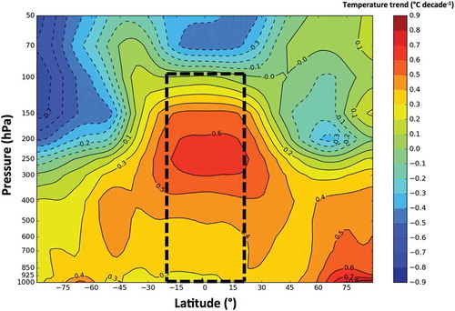
The bulk atmosphere, specifically the troposphere (the air from the surface to the stratosphere, or about 85% by mass), is an especially informative layer because it is anticipated to show the most pronounced bulk temperature response to greenhouse forcing (Christy and McNider 2017). In Figure 1 we show the vertical and latitudinal atmospheric temperature trend from a computer simulation of 1979–2016 to demonstrate this feature, common to climate model simulations, in which the upper air throughout the troposphere will generally warm more rapidly than the surface for the tropics and mid-latitudes (for other model results see Christy and McNider 2017). Because of the mass involved in the bulk troposphere, monitoring its average temperature provides a more representative answer to the question of how much heat is accumulating in the atmospheric climate system than would surface measurements.

Figure 1. Latitude – Altitude cross-section of 38-year temperature trends (°C decade⁻¹) from the Canadian Climate Model Run 3. The tropical tropospheric section is in the outlined box.

There is a relatively large body of literature related to the construction of tropospheric temperature datasets and how they are applied to issues of climate variability and change (e.g. Christy and McNider 2017; Santer et al. 2017; Hartmann et al. 2013; citations therein). The key points of uncertainty in these papers deal with the confidence one may have regarding the various construction techniques of the products, particularly how they impact the resulting trend magnitudes. This is important because as new versions of the datasets are produced, trend magnitudes have changed markedly, for example the central estimate of the global trend of the mid-troposphere in Remote Sensing System’s increased 60% from +0.078 to +0.125°C decade⁻¹, between consecutive versions 3.3 and 4.0 (Mears and Wentz 2016). Lower trends would suggest relatively modest sensitivity of the climate system to extra greenhouse gas forcing, while higher trends would support greater sensitivity. Thus, the trend magnitudes are critical, for example, to understanding the response of the climate system to enhanced forcing. In this paper, our focus will be on the credibility of the datasets and associated trends, suggesting reasons for their differences and offering a best estimate based on multiple, independent efforts.

The satellite-monitored layer for this study is commonly referred as the mid-troposphere (T_MT) because the peak of energy received by the satellite originates in the mid to upper troposphere with the main weighting function (96% of the signal) going from the surface to 70 hPa. Some stratospheric influence occurs, where trends are negative, especially outside the tropics, thus trends of T_MT will be slightly lower than trends of the troposphere alone.

In this study we shall examine the satellite, radiosonde and reanalyses datasets to assess their similarities and differences for the purpose of understanding how the global bulk-atmospheric temperature has fluctuated. We shall look at global comparisons of 564 stations of the Integrated Global Radiosonde Archive (IGRA) dataset as well as sub-sections (with number of stations in parentheses) as follows: 30°S-30°N (135, to accommodate one of the datasets), Australian radiosondes (34) and those produced for the United States by the VIZ Manufacturing Company (US VIZ) radiosondes (32). These latter two subsets have been studied extensively in the past, including by Christy, Spencer, and Norris (2011), hereafter C11, and will provide continuity with those studies. The reader is encouraged to access C11 for much of the background that will be briefly discussed herein.

We shall also examine T_MT as produced from homogenized radiosonde datasets and Reanalyses in the physically-coherent deep tropics (20°S-20°N). From this analysis, we shall briefly examine these tropical results by comparing them with 102 climate model simulations utilized in the Intergovernmental Panel on Climate Change Assessment Report 5 (IPCC AR5, Flato et al. 2013) and made available through the Koninklijk Nederlands Meteorologisch Instituut (KNMI) Climate Explorer (van Oldenbrogh 2016).

2. Satellite microwave and radiosonde observations of the bulk atmosphere

Since late 1978, the United States included microwave sounding units (MSUs) on board their polar-orbiting operational weather observation satellites. With the launch of the National Oceanic and Atmospheric Administration’s NOAA-15 spacecraft in 1998, a new instrument, the Advanced MSU (AMSU) began service that has continued to be placed into orbit by succeeding U.S. NOAA and National Aeronautics Space Administration (NASA) missions as well as those of the European Space Agency. For the layer discussed here (roughly the surface to 70 hPa), the radiometer on the MSU channel 2 and AMSU channel 5 measures the intensity of emissions, which is directly proportional to temperature, from atmospheric oxygen near the 53.7 GHz band (Spencer and Christy 1990). Data that have been utilized to generate the satellite time series have been provided from nine spacecraft that have carried the MSU (1979–2001+, the University of Alabama in Huntsville (UAH) ceases to use the last MSU in mid-2001, others through 2004) and six AMSU (1998-present). These spacecraft have been launched roughly every two or three years and usually have a multi-year overlap with previously-launched, on-orbit spacecraft so that intersatellite biases may be calculated and removed, producing a single time series.

Products from four groups who generate bulk atmospheric temperatures from satellites are available from which we are able to provide a substantial update to our previous work (C11). All datasets have been revised and are available as monthly gridded anomalies in new versions referred to as UAHv6.0, Spencer, Christy, and Braswell 2017), Remote Sensing Systems v4.0 (RSSv4.0, Mears and Wentz 2016), NOAAv4.0 (Zou and Wang 2011 plus website updates) and a new dataset, University of Washington v1.0 (UWv1.0, Po-Chedly, Thorsen, and Fu 2015). The datasets provide monthly gridded T_MT anomalies on a 2.5 degree near-global grid (85°S-85°N), though UW processes 30°S-30°N only.

Each group builds the datasets in different ways to account for (a) small calibration drifts once on orbit, (b) radiometer response fluctuations due to variable solar insolation on the instrument, (c) non-climatic temperature variations that occur when the spacecraft drifts east or west from a fixed local crossing time at the equator (diurnal drift), (d) intersatellite biases, and (e) loss of altitude due to frictional drag from the thin atmosphere. The publications cited above for the various satellite datasets delve into the details of how each group has decided to account for these influences and should be referred to if the reader has further interest.

The key metric that shows the greatest divergence among the satellite datasets is the linear trend over the period examined here (1979–2016), ranging among the datasets to as much as 50% from a central estimate in the tropics for example (see later). As noted in the introduction, the trend is a critical parameter to aid in understanding how the global, bulk atmosphere is responding to the extra forcing brought about by increasing concentrations of greenhouse gases. As such, we shall focus more on the trend as the metric of discussion because (a) it reveals the greatest discrepancies and (b) it is critical to the science issue of human-induced climate change.

A new update of a major radiosonde dataset from NOAA, IGRA v.2 or ‘IGRA’ with data through mid-2016, will be used as a source for independent comparisons (Durre and Yin 2011). Key updates to the IGRA dataset are (1) inclusion of data not found in IGRA v.1, (2) more convenient organization and formatting, (3) inclusion of derived parameters and (4) updates in station metadata. Most of the analysis below will utilize the period 1979–2015, but in a few cases will use 1979–2016 recognizing that the stations used here from IGRA, though containing the peak warm temperatures of early 2016, end in June 2016.

Unlike the satellite data that provide near-global coverage from a single instrument per satellite, IGRA radiosonde stations are scattered around the globe with greatest coverage over the northern midlatitude continents. Most stations release their balloons either once or twice a day (00 and/or 12 Coordinated Time Universal or UTC). From these daily data, microwave brightness temperatures are calculated and monthly averages are generated for each station. Ten days of data in the month are required for a monthly average to be calculated for each of the observation times. In many cases, only one of the release times (00 or 12 UTC) exceeded the days-per-month threshold, so several stations provided only one release time for their time series. If sufficient data were available from the two release times, the data were merged into a single time series after accounting for diurnal biases and differences in mean annual cycles. Otherwise, the time series consisted of data from only one release time. In all comparisons below, if a month were missing in the radiosonde data, it was set to missing in the satellite data so there would be no aliasing of means or annual cycles between the two data sources.

IGRA stations were accepted if at least 240 monthly observations were available (of the 450 possible in the Jan 1979 to Jun 2016 period.) Then, a final quality check was performed. If the monthly correlation of anomalies between the unadjusted station data and the satellite data at the corresponding gridpoint exceeded 0.70, the station was accepted for the comparison studies to follow. In general, correlations versus satellites for stations with fairly systematic data collection, but even with changes in instrumentation, were on average around 0.90, with many above 0.95. Of the 620 stations with 240 months of data, 56 failed this correlation test due to significantly erratic time series.

The IGRA station-by-station, (usually) twice-daily radiosonde data (temperature and humidity) on all reporting levels are vertically interpolated to 61 prescribed pressure levels for the calculation of the satellite temperature through a radiative transfer model based on Ellingson and Fouquart (1991, defining the pressure levels used) and Rosenkranz (1993) for the function code. These are then averaged into monthly values from which a mean annual cycle and anomalies are calculated. These are equivalent to the satellite-observed T_MT anomalies for direct comparison with the satellite temperatures at the station/grid-point (2.5°x2.5°) level.

2.1. Comparison methodology and adjustment procedure

We will show below both the direct comparison of IGRA vs. the satellite time series without any adjustment to any dataset as well as results using adjusted IGRA data. The non-adjusted result is the most independent of the comparisons to be shown which means that the differences in the time series may be due to radiosonde and/or satellite problems. Unfortunately radiosondes have undergone events which impact the time series, i.e. changes (improvements) in software, instrumentation, and factors such as cord length between the balloon and the instrument box. These changes are generally detectible as a shift in the time series (examples will be shown later). Unlike surface temperature stations that may suffer from slow temperature drifts due to gradual changes in the immediate surroundings for which adjustment is extremely difficult, radiosonde time series usually are composed of homogeneous segments at the endpoints of which are sudden shifts as a change is instituted (e.g. Christy et al. 2006; Christy, Norris, and McNider 2009; Haimberger 2007; Zhang and Seidel 2011). As a result, we are able to ‘detect’ a radiosonde change by examining the time series of differences between the radiosonde and satellite.

When a significant shift in the difference-time-series is detected (by the simple statistical test of the difference of two segments of 24-months in length on either side of the potential shift) we then adjust the radiosonde to match the satellite at that shift point. In the sections below we shall use a t-test value of 3.0 to detect and adjust for a shift (C11). Each satellite will be utilized to generate the shift points according to its own time series, thus ‘IGRA ADJ’ will be specific for each satellite dataset. Satellite time series will not be adjusted in anyway.

This adjustment procedure does not guarantee that the adjusted IGRA station time series is more correct. It is entirely possible that a detected shift may result from an issue with the satellite, for example when a new satellite is merged into the time series, there may be a shift introduced, especially on a regional scale. We are assuming that most of the shifts detected are indeed IGRA station issues but recognize that when such a shift is applied as a correction to the radiosonde, we are forcing an improvement in the agreement between the radiosonde and satellite in a contrived way. Because the satellites have varying methodologies of construction (UAH is especially different than the other three) this will provide more than one test of the radiosonde breaks.

A unique aspect of this study is the idea that each satellite dataset may be thought of as an independent ‘reference dataset’ relative to the radiosondes. By using identical methods to ‘correct’ radiosondes with differing satellite datasets, we will have multiple results for which common and disparate results may be forthcoming. For example, as will be shown later, there is a common result among all satellite datasets regarding trends vs. radiosondes in the 1990s which gives us confidence in its veracity.

2.2. Averaging

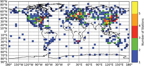
We shall present results in which the comparison data have been averaged for multi-station means. We gather the stations into 5° latitude x 5° longitude grid boxes, merge the anomalies of the stations (accounting for biases) and generate a single time series based on all stations in the grid box. However, recall that each individual station is adjusted relative to its corresponding 2.5° x 2.5° satellite gridbox time series before being placed into the 5° x 5° gridbox. For the global and sectional averages we then average the 5° latitude x 5° longitude time series into 5° latitude by 30° longitude grid boxes and compute the area-weighted global/sectional mean from there. We found that several grid boxes in populated regions contained 4 or 5 stations, so giving each of these the same weight as an isolated island station does not properly account for spatial characteristics of a large-region average (Figure 2). Hence the gridding process will have the advantage of providing a quantity that greatly reduces spatial inconsistencies.

Figure 2. Map of radiosonde locations on a 5° x 5° degree grid with number of stations indicated by color.

3. Results

3.1. Near-global results

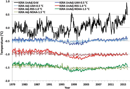
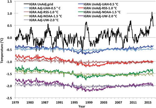
In the following we will show several metrics of comparison between IGRA and the satellite datasets with the goal of synthesizing what is discovered into an estimate of the true bulk atmospheric trends and offer evidence-based suggestions as to why the datasets differ. We begin with the global time series of the unadjusted IGRA data and subtract from that the equivalent satellite time series both unadjusted and with adjustments to IGRA (Figure 3). There were 564 IGRA stations which met the requirements for inclusion. In the top time series of Figure 3, IGRA UnAdj T_MT demonstrates the significant influence of El Nino/Southern Oscillation events with warm phases in 1983, 1987, 1990, 2005, 2007, 2010 and major ENSOs in 1997–98 and 2015–16. The differences between each satellite dataset and unadjusted and adjusted IGRA stations are shown as well.

Figure 3. Top: Time series of the unadjusted near-global anomalies of the IGRA radiosonde data (black). Thick Blue (UAH), Red (RSS) and Green (NOAA) time series are the differences (unadjusted IGRA minus satellite). Thin time series are the adjusted IGRA station data minus satellite time series.

To quantify the obvious differences between IGRA and the satellite datasets in Figure 3 we shall display statistical information in the following three figures. In Figure 4 we show the standard deviation of the difference-time series for unadjusted and adjusted IGRA station data. It is evident that the adjustment procedure has performed as anticipated and has considerably reduced the magnitude of the differences in all datasets. In the unadjusted and adjusted results, we see UAH produces the smallest differences, though in the adjusted results, RSS is only slightly greater.

Figure 4. Standard deviation (°C) of the monthly difference time series in Figure 3.

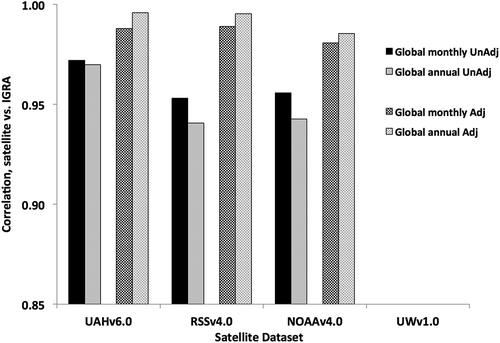
In an associated statistic, we show the correlations of IGRA, both monthly and annually, versus the various satellite time series in Figure 5. Here again, as anticipated, we find improved correlations in the adjusted data, with some above 0.99. However, recall that our adjustment procedure forces the IGRA stations to align with the satellite data at places where shifts are detected, but even so, the agreement is remarkable. We again remind the reader that we are demonstrating only relative agreement between time series since none of the products examined here may be considered to be an absolute reference standard. By way of approximation, using the Fisher r-to-z transformation for 100 degrees of freedom, differences are generally statistically different from one another for value above 0.9 if the lower value is of a magnitude smaller than the difference between the higher value and 1.0. So, for example, two correlations of 0.98 and 0.95 are statistically different since the difference between 0.98 and 0.95 is greater than the difference between 1.00 and 0.98. In Figure 5, the various correlations approach significant difference relative to UAH, but do not reach it. That UAH demonstrates higher levels of agreement with IGRA may simply be due to unrelated but common errors in both, though we shall offer some explanations below.

Figure 5. Monthly and annual correlation of global anomalies between the unadjusted and adjusted IGRA time series and that of the satellites.

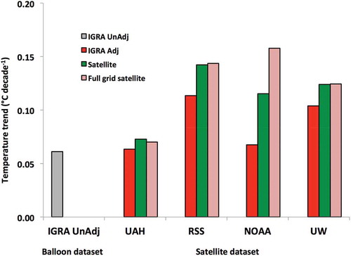
The third statistical metric, and physically most important, is the linear trend, and is displayed in Figure 6. We include the satellite trend that is calculated from the full (complete) satellite grid for the section (near-global here) to compare with those which are calculated from satellite grids in which IGRA stations exist. The general result here is that the full grid trends, which include more oceanic area, tend to be lower than the partial IGRA grid except for NOAA whose relative trends over oceans are more positive than that indicated by UAH and RSS (see later).

Figure 6. Linear trend (°C decade⁻¹) of the various global time series for 1979–2015. The ‘Full grid satellite’ trend is the trend of the satellite data at all grids (i.e. complete coverage), whereas ‘satellite’ is the trend based on IGRA station grids only (i.e. partial coverage).

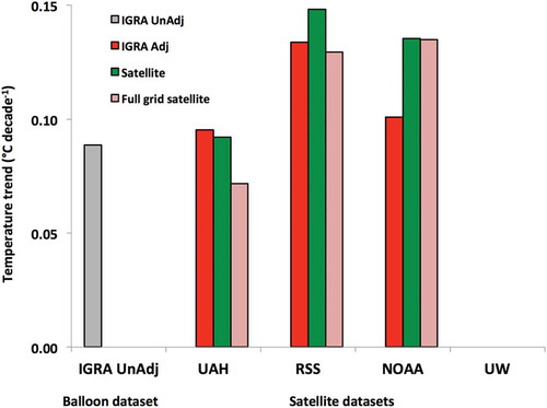
The unadjusted IGRA time series indicate closest agreement with UAH and thus little overall change is generated when adjusted even though the IGRA stations were individually adjusted, some considerably. RSS and NOAA satellite trends are much more positive than the unadjusted IGRA trend and so their adjusted IGRA time series become more positive, though for NOAA, the adjusted trend is within +0.01°C decade⁻¹ of UAH.

The difference-times-series (Figure 3) reveal useful information. Common to all unadjusted difference time series (thicker time series) is a relative warming in the satellite data vs. IGRA for the period 1990–2000. This is followed by a similar, though of lesser magnitude (except UAH), relative satellite cooling from 2003 to around 2006. We show the magnitudes of these differences in Table 1 in which we have computed the differences between relatively stable periods. UAH data reveal the least amount of relative warming between the first two periods and the most relative cooling between the second two periods in nearly all cases.

Table 1. Relative segment differences (°C) in the satellite comparison with unadjusted and adjusted IGRA data for globe and 30°S-30°N section. Periods are (1) 1979–1990, (2) 2000–2003 and (3) 2006–2015. Thus ‘(2)-(1)’ indicates the average of 2000–2003 minus the average of 1979–1990. The first value for UAH is +0.116°C meaning UAH warmed +0.116°C more than IGRA UnAdj between the two periods 1979–1990 and 2000–2003. The adjustments are unrestricted, i.e. the satellite alone determines all breakpoints based only on the breakpoint detection scheme.

	GL (°C)		30°S-N (°C)			GL (°C)		30°S-N (°C)
UnAdj	(2)-(1)	(3)-(2)	(2)-(1)	(3)-(2)	Adjusted	(2)-(1)	(3)-(2)	(2)-(1)	(3)-(2)
UAH	+0.116	−0.114	+0.144	−0.121		+0.017	−0.025	+0.031	−0.005
RSS	+0.248	−0.111	+0.294	−0.108		+0.056	−0.019	+0.067	+0.010
NOAA	+0.204	−0.101	+0.211	−0.092		+0.087	+0.003	+0.114	+0.011
UW			+0.318	−0.187				+0.084	−0.033

As can be seen in the ‘Adjusted’ results of Figure 3 and Table 1, the shift-point adjustment procedure eliminates most of the two main discrepancies, though it is applied to each radiosonde independently. Even so, the first drift in the difference time series in 1990s retains some magnitude (Table 1) in the adjusted data, especially for the non-UAH datasets. As will be discussed later, this drift is hypothesized to be a consequence of spurious warming in the NOAA-12 and −14 processed satellite data and not spurious cooling in the IGRA radiosondes.

3.2. 30°S – 30°N

With the 30°S-30°N latitude band we now bring in UW data into the comparison study where for this region there are 135 stations to examine. In Figure 7 we show the low-latitude time series as described in Figure 3 and which depicts similar features – the relative warming of satellites from about 1990–2000 and relative cooling 2000–2006. More obvious here is the various amounts of relative cooling from the satellites in post-2011 unadjusted IGRA data, least for RSS and most for NOAA. These differences are eliminated in the adjusted data.

Figure 7. As in Figure 3 above but for stations in 30°S-30°N and now includes UW (purple).

The magnitude of the correlation of the anomalies (Figure 8) is highest for UAH, though in the adjusted-IGRA data, UAH, RSS and UW are statistically indistinguishable. Figure 9 displays the trends for this latitude section and as was true in the case of global average, the IGRA-adjusted NOAA and UAH (red) values are very similar to the IGRA-unadjusted. RSS and UW introduce more significant shifts to IGRA, adding approximately +0.05°C decade⁻¹ to the unadjusted value. The adjusted IGRA trends for all satellites are less positive than those of the satellite to which they have been tuned, which may be explained by residual relative drifts in the satellite data during periods when there are no breakpoints to detect (C11). One additional observation to note is, as mentioned earlier, that NOAA’s trend of the ‘full grid’ (pink) is much more positive than its trend calculated from only the IGRA grids (green) while the other three datasets are virtually the same (within ±0.003°C decade⁻¹). This essentially indicates more positive trends over the ocean than land in NOAA and is a peculiarity not found in any of the other datasets.

Figure 8. Correlations with IGRA values as in Figure 5 above but for 30°S-30°N and now includes UW.

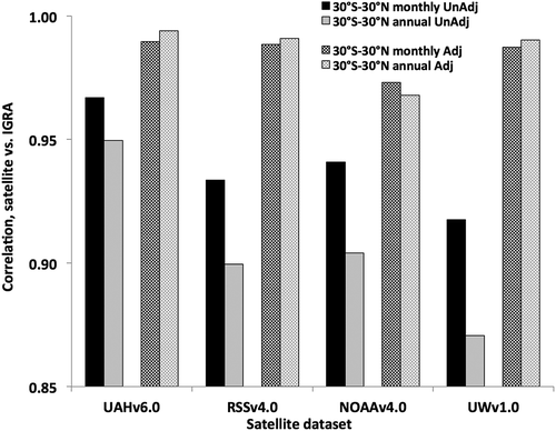
Figure 9. As above in Figure 6 but for 30°S-30°N.

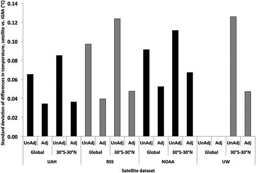
In support of the information in Table 1 we show in Figure 10 the relative difference over the periods between satellites and homogenized radiosonde datasets provided by different institutions (satellite values were calculated from grids containing radiosonde data). The result is clear that RSS, NOAA and UW experience significant warming relative to the homogenized radiosonde datasets and reanalyses between 1990 and 2000. This is further and substantial evidence that the satellite time series are characterized by spurious warming in the 1990s. [We note again the peculiarity of the oceanic warming in the NOAA dataset in that the relative differences between NOAA and the homogenized radiosonde datasets appears less than that of RSS and UW (Figure 10 left three comparisons) whereas it is greater for the reanalyses comparison. This is so because NOAA’s high warming rate over the oceans is not captured in the grid-matched homogenized radiosonde comparisons whereas the Reanalyses are full-grid in the datasets, and thus include the oceans.]

Figure 10. Magnitude of the relative difference between two periods for the respective satellite datasets (colored bars) and the respective radiosonde-based datasets (i.e. positive value indicates satellite warmed more than the radiosonde-based data between defined periods.).

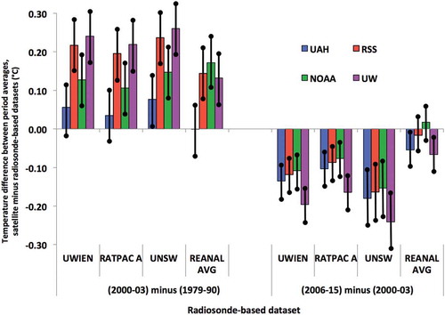
Figure 10 also supports the idea that the homogenized radiosonde datasets (as shown below for Australian and VIZ stations) are likely characterized by spurious warming after 2000. We see close agreement between the satellite datasets and the Reanalyses for the differences between the latter two periods ((2006–2015) minus (2000–2003)) yet significant differences for all satellite datasets vs. the homogenized radiosonde datasets. While not definitive, these results and those below suggest spurious post-2000 warming in the radiosondes (that is largely eliminated in our adjustment process, see Table 1 far right column.)

3.3. Australia stations

In this and the following section (3.4 U.S. VIZ) we look more closely at the comparisons between radiosondes and satellites because there is a body of research that includes considerable meta-data regarding the instrumentation and software of the radiosonde observations for these two nations each of which has wide geographical coverage (tropics to polar latitudes) with one in each hemisphere. With such information, we will have the opportunity to make hypotheses about potential satellite problems. We begin with Australian radiosondes for which we have clear evidence of positive shifts due to instrumentation changes (Christy and Norris 2009, C11). These changes were not simultaneous across the network, so we continue to utilize the single-station adjustment procedure as used above, i.e. allowing each satellite dataset to detect the shifts. In this comparison, we have reduced the longitudinal dimension to 10° while retaining the 5° latitudinal spacing. There were 34 stations in the sample that met the criteria for all of Australia-controlled stations and 18 for the region north of 30°S for UW comparisons.

For the 34-station network, all three of the correlations of the adjusted IGRA data were between 0.98 and 0.99 for annual anomalies (not shown). Unadjusted annual correlations were 0.915, 0.916, and 0.865 for UAH, RSS and NOAA respectively. For the 18-station network in the low latitudes (north of 30°S), the four satellite datasets produced annual correlations of unadjusted (adjusted) IGRA data of 0.891 (0.984), 0.916 (0.972), 0.889 (0.976) and 0.847 (0.957) for UAH, RSS, NOAA and UW respectively.

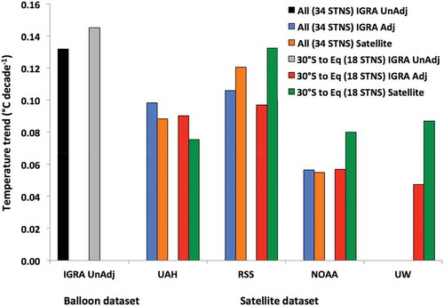
Of most interest is the information on trends shown in Figure 11. As expected from previous research (Christy and Norris 2009), the unadjusted Australian data (black and gray) indicate more positive trends than any dataset. We note that when UAH and RSS are used to adjust the radiosondes the resultant time series have very similar trends, within 0.01°C decade⁻¹ of each other in both cases (blue and red). Adjustments applied utilizing NOAA and UW for breakpoint detection produce very similar magnitudes with each other and are more substantial, i.e. producing a less positive adjusted trend than when using UAH and RSS. NOAA’s satellite trend for the 34-stations is considerably less than UAH and RSS (orange), hence when applying adjustments, will produce a less positive result.

Figure 11. Trends (°C decade⁻¹) for the various time series using Australian stations only.

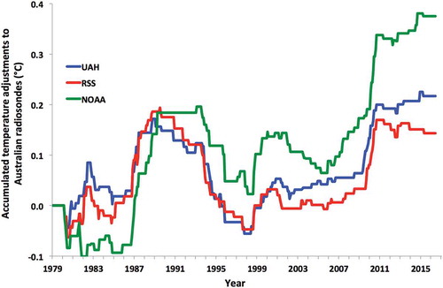
In an attempt to understand Figure 11, we show the net accumulation of the breakpoints detected by each satellite for the 25 Australia stations with > 400 months reporting in Figure 12. The three main features are the detection of (a) a radiosonde warming shift in the late 1980s, (b) a gradual radiosonde cooling period in the 1990s, and (c) a radiosonde warming shift in late 2009 and early 2010 (confirmed by comparisons with the European Centre for Medium-range Weather Forecasts analyses, L. Haimberger personal communication). UAH and RSS are highly consistent in their detection rates and magnitudes, with their time series correlating at +0.93. NOAA is less consistent, correlating with UAH and RSS at +0.79 and +0.73 respectively. The trends of the accumulated adjustments are +0.03, +0.02 and +0.10°C decade⁻¹ for UAH, RSS and NOAA respectively. The detection of a gradual radiosonde cooling trend in the 1990s is evidence of spurious warming in the satellites during the 1990s, as discussed below, as there were essentially no changes in the instrumentation between 1991 and 2000. In other words, the satellites appear to detect breakpoints more or less randomly due to their spurious warming rather than to spurious cooling in the radiosondes. That NOAA detects fewer of these in the period appears to be related to the lower correlation of NOAA vs. radiosondes so that the significance level is not achieved as often to apply a breakpoint shift adjustment.

Figure 12. Net accumulation of breakpoint magnitudes (°C) for 25 Australia stations with > 400 months of data. This may be interpreted as an index of the relative difference between the raw Australian data and the satellites, showing a relative warming vs. the satellites.

3.4. U.S. VIZ stations

A decision was made in NOAA’s weather observing strategy before the 1980s to set aside several radiosonde stations for which, as much as possible, a consistent set of instruments and software would be maintained so as to create climate data records suitable for long-term studies. These stations utilized the VIZ radiosonde, but as improvements were naturally forthcoming through the years, these stations indeed adopted new instrumentation from the same manufacturer but with as much backward compatibility as possible (Christy and Norris 2006). Unlike the Australia network, changes to the VIZ network were usually near-simultaneous and thus easily spotted using the composite time series when checking for shifts (see examples in C11). As with the Australian study we shall bin the data into 10° longitude x 5° latitude cells.

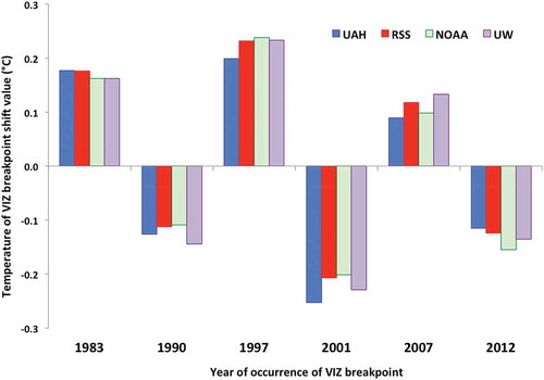
Christy and Norris (2006) identified four shifts due to instrument or software changes between 1979 and 2004, occurring in (a) mid-1983, (b) end-1989, (c) mid-1997 and (d) end-2001. To this list, with data to mid-2016 now, the comparison against all satellite datasets indicate two additional, significant shift points (a) 2007 (when the instruments switched to Global Positioning System (GPS) tracking) and (b) late 2012 (cause unknown as metadata not updated through this date). There is a possibility that introducing the data from the Meteorological Operational (METOP) spacecraft launched by the European Organization for the Exploitation of Meteorological Satellites in 2012 (METOP-B) may have caused a spurious shift in the satellite data. However, UAH performed the test with and without METOP-B, yet detected the shift with as much significance as the other satellite datasets both ways, so it is unlikely that the addition of METOP-B (i.e. a satellite issue) caused the shift.

In this analysis we shall apply corrections only at these six shift points, the value of which will be determined by each satellite dataset. This is a more restrictive test than previous tests because with the earlier tests, all shift-points were accommodated without any knowledge of which dataset, IGRA or satellite, might have created the error. In this test, we are essentially certain that the IGRA data requires adjustment and we shall not allow other shift-points to be applied, assuming they are likely due to satellite problems. As such, this test will have the potential of identifying problems with the satellites more directly. We shall again divide the analysis into two groupings (1) all 32 stations for UAH, RSS and NOAA, and (2) 12 stations within the 30°S-30°N band to allow direct comparison of all satellite datasets with UW.

In Figure 13 we show the adjustments applied to the composited VIZ stations as determined by the satellite data (for low latitudes). Generally speaking the individual shift-point values are slightly more positive for RSS and NOAA than UAH and UW, but overall are quite consistent among the satellite datasets. It is interesting to note that the accumulation of these adjustments is −0.03, +0.08, +0.03 and +0.02 for UAH, RSS, NOAA and UW which is consistent with the less positive trend of UAH and the higher trend of RSS.

Figure 13. Values of the shift magnitude (°C) added to the 12 tropical/subtropical IGRA VIZ radiosondes from the indicated time forward.

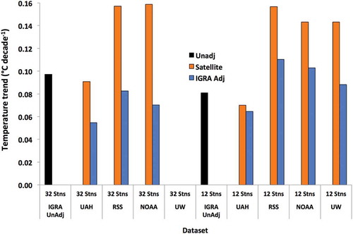
The correlations of monthly and annual anomalies are shown in Figure 14 for adjusted (pink and red) and unadjusted (black and gray) IGRA data. In all cases, UAH data demonstrate higher levels of agreement and UW the lowest with RSS and NOAA producing similar values. As noted earlier, the Fisher z-to-r transformation indicates the monthly correlations of RSS, NOAA and UW are near or just significantly less than UAH for all results. The trend magnitudes are shown in Figure 15. In all cases the adjusted trend (blue) of the 32-station composite is less than the unadjusted radiosonde trend (orange.) We note that the more positive trend values of the satellites (less so in UAH) indicates relative trend differences during periods without radiosonde changes, in particular as shown below, the period of the 1990s.

Figure 14. Correlations of monthly and annual anomalies, unadjusted and adjusted between US VIZ stations and the four satellite datasets, Jan 1979 – Jun 2016.

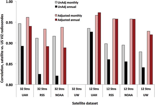
Figure 15. Trend magnitudes (°C decade⁻¹) utilizing the US VIZ radiosonde stations as adjustment data for 1979–2015.

We focus now on an issue raised in previous research (C11) that suggested the MSUs during the 1990’s exhibited a spurious warming drift that was unexplained and (mostly) untreated by the satellite dataset providers. In Figure 16 we show the annual anomaly time series of the IGRA data for low-latitude US VIZ stations with the difference time series (IGRA-adjusted minus satellite) below. As the mean of all of the radiosonde minus satellite time series indicates, the largest departure from a flat difference series is the relative warming of the satellites between 1990 and 2000. There appear to be two other smaller differences, a slight relative satellite cooling in the early 1980s and after 2000.

Figure 16. Time series of the composite of annual anomalies of IGRA US VIZ and the difference (°C) versus the four satellite datasets for the 12 low-latitude stations.

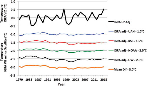
We shall return to this topic in the discussion section, but here provide statistical results. Taking only data from VIZ radiosondes for which no instrument or software changes were applied (Jan 1990 to Jun 1997), we find the satellites warm relative to radiosondes with a significant magnitude when comparing the 48 months before and after this period (mean satellite shift of +0.13°C.) After including the correction for the Jul 1997 VIZ shift (due to change from VIZ–B to VIZ-B2 instrumentation), the mean satellite shift for the period Jan 1990 to Dec 2000, was +0.18°C. Thus the evidence is strong that NOAA-12 and −14’s MSUs were characterized by a spurious warming drift, as also seen in the independent set of Australian radiosonde analysis above. We note that this feature is also present in the global and tropical time series (Figure 3, 7), which involves the full IGRA dataset with numerous radiosonde stations. We note too that for the longer period tested, the magnitude of the relative drifts were smallest for UAH, especially in the low latitude stations and likely due to the unique way UAH merged this section of the time series (see later). Given these results, we estimate the actual global (full grid, Figure 6) T_MT trend to be +0.10 ± 0.03°C decade⁻¹, i.e. a value slightly less positive than satellite datasets on average indicate.

3.5. Other tropical T_MT datasets (20°S-20°N)

Before moving to a synthesis and analysis of the results above we include one more test involving homogenized radiosonde and reanalyses datasets. These datasets in various ways seek to remove temporal inhomogeneities independently from any process performed in this paper. For simplicity we will consider annual anomalies of the deep tropics (20°S-20°N) for which Figure 1 indicates is a region of significant response to generic forcing of the troposphere of any kind with upper air warming faster than the surface. In terms of magnitude, when comparing surface and T_MT warming rates since 1979, the theory, as indicated by model simulations, reveals that the rate of warming in the T_MT layer is an amplification of the surface warming rate by a factor of 1.4 (Christy 2017.)

There are four homogenized radiosonde and three Reanalyses datasets described in Christy (2017) and listed in Table 2. The radiosonde datasets represent the homogenization processes of the associated authors in which adjustments are calculated and applied in different ways to the individual station records. The reanalyses represent an assimilation of all available data, including radiosonde and microwave satellite data used here, into a global general circulation model. (We note that University of Wien (UWien) radiosonde datasets are indirectly interdependent with European Reanalysis European Centre for Medium Range Forecasts Reanalyses-Interim (ERA-I) reanalyses, (Haimberger 2007) The assimilation process aids in identifying and then accounting for spurious changes in the various observing systems. It is clear that each of the radiosonde and reanalyses are independently constructed.

Table 2. Datasets utilized in the comparison of tropical (20°S-20°N) T_MT statistics.

Dataset	Type	Source Citation
IGRA Grid UnAdjusted	Radiosonde	Durre and Yin, 2011 and this paper
IGRA Grid Adjusted	Radiosonde	Durre and Yin, 2011 and this paper
UWien	Radiosonde	Average of RAOBCORE and RICH
RAOBCOREv1.5	Radiosonde	Haimberger, Tavolato, and Sperka 2012
RICHv1.5	Radiosonde	Haimberger, Tavolato, and Sperka 2012
NOAA/RATPAC-A2	Radiosonde	Free et al. 2005
UNSW	Radiosonde	Sherwood and Nishant 2015
ERA-I	Reanalyses	Dee et al. 2011
JRA-55	Reanalyses	Kobayashi et al. 2015
MERRA-2	Reanalyses	Bosilovich et al. 2017

IGRA: Integrated Global Radiosonde Archive.

UWien: University of Wien.

RAOBCORE: RAdiosonde OBservation COrrection using Reanalyses.

RICH: Radiosonde Innovation Composite Homogenization.

RATPAC: Radiosonde Atmospheric Temperature Products for Assessing Climate.

UNSW: University of New South Wales.

ERA-I: European Centre for Medium-Range Weather Forecasts, Reanalysis – Interim.

JRA-55: Japanese 55-year Reanalyses.

MERRA-2: Modern-Era Retrospective-Analysis for Research and Applications v. 2.

We next examine the central estimate of the trend metric for these products (Figure 17). IGRA trends are calculated through June 2016 (the end of the IGRA-2 dataset) which included the peak warming in Feb 2016 from the El Niño event. [Note that for IGRA-Adj we include a bracket to show the range of the adjusted trends from the four satellite products (+0.056 to +0.124°C decade⁻¹).] The IGRA UnAdj trend is clearly lower than the others, though only slightly, and indicates that the net impact of adjustment procedures is to increase the trend. This is due in part to a common improvement to many (not all) of the radiosonde instrument packages through the years in which shielding of the direct sunlight, which had caused excessively warm temperatures in the upper troposphere and stratosphere in the early years in some models, was made more effective (e.g. Sherwood and Nishant 2015). Because T_MT has a portion of its signal from the upper troposphere and lower stratosphere, such an improvement would increase the trend relative to no adjustment applied.

Figure 17. The central estimate of the trend magnitudes (°C decade⁻¹) for T_MT, 20°S-20°N for several datasets described in Table 2. The IGRA Adj range represents the low to high values as adjusted by the four satellite datasets.

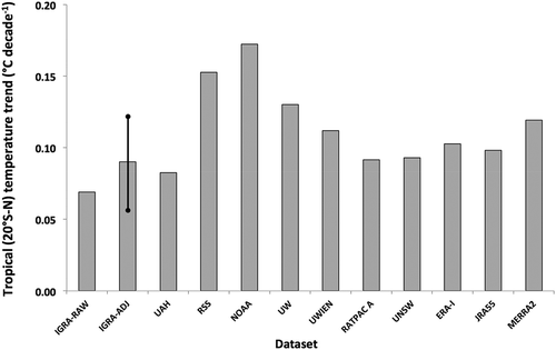
The results of Figure 17 indicate that the trend of the products not exclusively based on satellite data (and without IGRA UnAdj) cluster around +0.10°C decade⁻¹. Indeed, the trend calculated by generating a time series of the annual average of anomalies using the 8 products (counting the mean of IGRA-Adj as one of the samples) is +0.103°C decade⁻¹ with a standard deviation among the trends of 0.0109°C. Determining the error bounds is not straight-forward, but though we know each product was independently constructed, the use of common data likely removes some degrees of freedom (d.o.f.). With that in mind we select a t-test value calculated for 5 d.o.f. providing a confidence interval of ±0.028°C decade⁻¹, or a spread of +0.075 to +0.131°C decade⁻¹. Such a range marginally captures UAH on the low side (+0.082) and UW on the high end (+0.130). Note that the range of the IGRA-adjusted trends from the four satellites is very similar to this. Thus, (naively) applying the statistical results here we conclude that the central estimates of RSS (+0.153) and NOAA (+0.172°C decade⁻¹) are significantly different from the T_MT trends calculated by major international efforts. We say ‘naively’ because we cannot reject a hypothesis that the results from this diverse set of data providers who use a diverse set of methods may all be affected by common spurious cooling problems.

We tested the 20°S-20°N trends of each satellite time series against the average of the homogenized radiosonde datasets (UWien, Radiosonde Atmopsheric Temperaure Produces for Assessing Climate or RATPAC, University of New South Wales or UNSW) and the average of the reanalyses (ERA-I, Japanese 55-year Reanalyses or JRA-55 and Modern-Era Retrospective analysis for Research and Applications version 2 or MERRA-2) in Table 3. Trend differences between radiosondes and reanalyses are due to the subsampled grid for the homogenized radiosonde datasets. The trend of the satellite datasets may be thought of as the central estimate of the time series around which errors are distributed. We find that the difference trend for time series beginning in 1979 and ending in 2005 (covering the period of hypothesized satellite warming – see Table 1) is significantly more positive than that of either of the composite comparisons for RSS, NOAA and UW.

Table 3. Trend magnitudes and 95% confidence intervals of the time series of the differences between the satellite datasets (SAT) and the average of the homogenized radiosonde datasets (RAOB: UWien, RATPAC-A2, UNSW) and the average of the Reanalyses (REAN: ERA-I, JRA-55, MERRA-2). (Personal Communication, R. McKitrick.) The period is 1979–2005 (capturing the period using MSU instruments) and the geographic extent is 20°S-20°N (see Figure 10). Units are °C decade⁻¹ with bold values indicating the central estimate of the satellite trend is significantly more positive than the comparison dataset.

1979–2005	Trend SAT minus RAOB (°C decade^−1)	Trend SAT minus REAN (°C decade^−1)
UAH	+0.045 ± 0.066	−0.008 ± 0.039
RSS	+0.116 ± 0.070	+0.066 ± 0.049
NOAA	+0.111 ± 0.069	+0.091 ± 0.053
UW	+0.117 ± 0.069	+0.064 ± 0.040

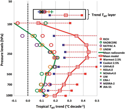
We conclude this section with an important comparison of the products shown here with the output of the IPCC AR5 climate models (from the Climate Model Intercomparison Project 5 or CMIP-5, Flato et al. 2013) using Representative Concentration Pathway 4.5. These simulations were forced with estimates of the actual forcing due to volcanic aerosols, greenhouse gasses, etc. through 2006 then estimates of these forcings thereafter, so were anticipated to reproduce fairly closely the global and tropical-scale temperature changes to this point. There were 102 simulations available which were grouped into 32 time series according to institution and model type. Simulations from institutions that provided multiple simulations were averaged for a single time series, so the results and statistics are based on a sample of 32 model time series. The satellite temperatures were calculated from temperatures at 17 pressure levels of model output using a static weighting function identical to that used for the homogenized radiosonde time series.

We show the results in Figure 18 for the metric of most interest, the trend over the period 1979–2016. The vertical pressure-level trends form the main part of the diagram and in the upper box is the single value of the T_MT trend for the various datasets discussed above. The main result here is the high value of trends in the simulations (average for T_MT is +0.27 ± 0.11°C decade⁻¹) is significantly above the estimates from observations (+0.10 ± 0.03°C decade⁻¹).

Figure 18. Trend magnitudes (°C decade⁻¹) from radiosonde and CMIP-5 climate model simulations over the period 1979–2016. In the upper box are the trend magnitudes of the T_MT layer as calculated by the various datasets defined in Table 2 and in this paper.

4. Discussion

We now discuss our results and offer some suggestions to explain the differences among the satellite datasets and provide estimates of the bulk atmospheric temperature trends. We begin with a key result that affects all satellite data to some extent.

4.1. Satellite warming in the 1990s

We have shown substantial evidence to support the hypothesis that the satellite datasets experienced spurious warming during the period that began with NOAA-12 and ended with NOAA-14 (1990–2001+) that could not be explained by the processes already addressed. The evidence is seen in (a) the full IGRA comparisons in both global and low-latitude regions, (b) the more controlled analysis using the US VIZ and the Australian radiosondes separately (both global and low-latitude) and (c) the comparison with Reanalyses and independently-constructed, homogenized radiosonde datasets. The impact is least obvious in UAH data and most in UW (Tables 1, 4) – e.g. note from Table 4 (30°S-30°N, 12 stations) the relative difference vs. adjusted US VIZ for 2000–2003 minus 1979–1990 was; +0.08, +0.19, +0.19 and +0.25°C for UAH, RSS, NOAA and UW respectively.

Table 4. As in Table 1 except using the 32 US VIZ radiosondes and fixed dates of breakpoint shift adjustments: segment differences in the satellite comparison with unadjusted and adjusted US VIZ data for full 32-station network and 30°S-30°N for the 12-station network. Periods are (1) 1979–1990, (2) 2000–2003 and (3) 2006–2015. The adjustments are those using the defined breakpoint events (breakpoints due to known/likely VIZ radiosonde changes).

StationUnAdj	(2)-(1) 32 Stns (°C)	(3)-(2) 32 Stns (°C)	(2)-(1) 12 Stns (°C)	(3)-(2) 12Stns (°C)	Defined Adjustment	(2)-(1) 32 Stns (°C)	(3)-(2) 32 Stns (°C)	(2)-(1) 12 Stns (°C)	(3)-(2) 12 Stns (°C)
UAH	+0.104	−0.122	+0.105	−0.138		+0.147	−0.044	+0.082	−0.055
RSS	+0.266	−0.119	+0.281	−0.091		+0.250	−0.055	+0.186	−0.058
NOAA	+0.270	−0.122	+0.287	−0.139		+0.262	−0.029	+0.193	−0.085
UW			+0.293	−0.143				+0.248	−0.104

We will discuss a merging detail here to help explain the discrepancies, though the reader is encouraged to consult the original papers. In the period of interest (1990–2000), we note that NOAA-11 (1988–1994) and −14 (1995–2001+) were ‘p.m.’ orbiters in which the spacecraft was inserted into an orbit with nominal local equatorial crossing time (LECT) of 1330 and with a purposeful drift toward later times in the afternoon to avoid backing into local solar noon. NOAA-10 (1987–1991), −12 (1991–1998) and −15 (1998–2008+) were ‘a.m.’ orbiters with nominal LECT of 0730. In general, a.m. orbiters drifted much less than p.m. orbiters. In particular, NOAA-14 drifted well away from 1330, being at 1700 by mid-2001 and 2030 (7 hours of drift) by the end of 2004. This was a far greater continuous drift than utilized in the other p.m. satellites and part of the reason UAH truncates NOAA-14 in mid-2001.

In the construction process, once the adjustments for diurnal drift and other issues were applied, in both UAH and RSS products, NOAA-14 revealed a trend that was about +0.2 °C decade⁻¹ more positive relative to NOAA-15, a spacecraft carrying the new and more carefully calibrated AMSU (Mo 2009). At this point UAH applied an objective algorithm to calculate and remove trend differences of NOAA-11 and −14 relative to the three a.m. orbiters, NOAA-10, −12 and 15 (Spencer, Christy, and Braswell 2017). This was done because these residual trend differences were very likely due to the changing impact of solar heating on the relatively rapidly drifting p.m. instruments. With the truncation of NOAA-14 data in 2001 and the trend adjustment based on simultaneous comparison with NOAA-12 and NOAA-15, the NOAA-14 trend difference in UAH data was considerably reduced. NOAA-12 was not impacted, however, as it was assumed to be stable. The fact that the US VIZ comparison indicates the relative warming of the satellites begins with NOAA-12 is a strong indication that it too was characterized by a spurious warming trend that was not accounted for in the UAH trend adjustment. In any case, this adjustment procedure is a partial explanation for the result that relative to the other satellite datasets in nearly all comparisons, UAH correlates highest, has the lowest magnitude of differences and the least difference in trends.

On the other hand, RSS (and likely NOAA and UW in some manner) choose to retain the relatively warm trend of NOAA-14, which they termed an ‘unexplained mystery’ (Mears and Wentz 2016). This, combined with a likely spurious warming of NOAA-12, produces the effect of ‘lifting’ the post-NOAA-14 time series up, producing a more positive trend.

As an experiment, Mears et al. recalculated the RSS overall trend by simply truncating NOAA-14 data after 1999 (which reduced their long-term trend by 0.02 K decade⁻¹). However, this does not address the problem that the trends of the entire NOAA-12 and −14 time series (i.e. pre-2000) are likely too positive and thus still affect the entire time series. Additionally, the evidence from the Australian and U.S. VIZ comparisons support the hypothesis that RSS contains extra warming (due to NOAA-12, −14 warming.) Overall then, this analysis suggests spurious warming in the central estimate trend of RSS of at least +0.04°C decade⁻¹, which is consistent with results shown later based on other independent constructions for the tropical belt. Details of the merging procedure of NOAA and UW are not known to this detail, but possibly are influenced in the same way. Differences in the diurnal correction may be important as well as discussed below.

There are substantial differences in dataset construction that separates UAH from the others that impacts trends. One is the diurnal correction. UAH determines corrections for the drift of the spacecraft through the diurnal cycle using empirical evidence only, i.e. intercomparing diurnally-drifting vs. non-diurnally-drifting satellites to calculate the effect directly. RSS and NOAA apply climate-model-calculated values which are evidently not sufficiently satisfactory (Mears and Wentz 2016; their Figure 7) while UW uses a numerical regression technique on residual differences between co-orbiting satellite pairs (both of which may be drifting) which also contains remaining ‘biases’ (Po-Chedly, Thorsen, and Fu 2015; their Figure 2.) RSS and NOAA then apply an additional step of ‘optimization’ required to compensate for the initial attempt to accommodate diurnal cycle errors. For example, the NOAA-14 satellite after diurnal correction over land from the climate model alone in RSS data, retained a trend relative to the co-orbiting NOAA-15 of +0.34°C decade⁻¹. The ‘optimization’ process reduced this discrepancy considerably to +0.20°C decade⁻¹ as noted above (Mears and Wentz 2016). Similar procedures were followed in NOAA and UW. This two-step method creates some differences in trends relative to UAH but it is clear that the attempted adjustment through a climate model was sufficiently erroneous that further adjustments were required. It is possible that a correction applied to a deficient correction may not lead to greater accuracy.

4.2. Satellite cooling in 2000’s

The relative cooling of the satellite datasets versus IGRA from 2002 to 2006 is more difficult to explain because once adjustments are applied, including the defined breaks of US VIZ radiosondes, the differences largely disappear (see Tables 1, 4). The main shift in the US VIZ is known for 2002 and once adjusted, the issue is mostly resolved. However, even after adjustment UAH retains a noticeable relative cooling trend of unknown origin during and following this episode which is also seen in NOAA and UW. We examined the satellites in question (NOAA-15 and AQUA) and found them to have a high degree of agreement (AQUA required no adjustments as it was a spacecraft restricted to a constant LECT.) The evidence from all satellite datasets suggests that the relative radiosonde warming during this period may be due to changes in a sufficient number of radiosonde stations to affect a global average. Even so, the comparative evidence (section 3.5) still suggests that UAH retains a spurious cooling trend after 2002 that likely introduces a relative negative influence of a magnitude of about −0.02°C decade⁻¹ on the complete time series.

4.3. Tropical trends, 20°S-20°N

The issue of tropical trends introduced in Figure 1 is especially important for understanding the theory of the atmospheric response to increasing concentrations of greenhouse gases. With the inclusion of independently homogenized radiosonde datasets; UWien (average of RAOBCORE and RICH), NOAA, and UNSW, and the reanalyses from major data-construction centers; ERA-I, JMA, and MERRA-2, we have more confidence in our conclusions. Figure 16 displays the 1979–2016 trends for the tropics (20°S-20°N). The IGRA-ADJ represents the trend of the mean of the IGRA stations adjusted for breakpoints by the four satellite datasets with the error bar indicating the spread of the results.

The median trend of the non-satellite-only (radiosondes and Reanalyses) datasets is +0.098 and including the satellite datasets is +0.103°C decade⁻¹. As noted earlier, one may conclude that the tropical T_MT trend is +0.10 ± 0.03°C decade⁻¹ based on difference statistics of the non-satellite-only data. This result suggests, again, that RSS and NOAA (in particular) are impacted by extra warming, especially in the NOAA-12 to −14 satellite period, to the extent that their overall central-estimate of the trend exceeds that produced in independent methods by a significant margin. We repeat an underlying fact here however, that these results may be viewed as strongly suggestive but not definitive as there is no true reference with which trend-precision may be determined. [The use of Australian and US VIZ radiosondes during periods without instrument changes is perhaps as close as we are able to approach such a reference at this time, and that analysis supports this hypothesis.]

4.4. General remarks

When examining all of the evidence presented here, i.e. the correlations, magnitude of errors and trend comparisons, the general conclusion is that UAH data tend to agree with (a) both unadjusted and adjusted IGRA radiosondes, (b) independently homogenized radiosonde datasets and (c) Reanalyses at a higher level, sometimes significantly so, than the other three. We have presented evidence however that suggests UAH’s global trend is about 0.02°C decade⁻¹ less positive than actual. NOAA and UW tended to show lower correlations and larger differences than UAH and RSS – indeed UAH and RSS generally displayed similarly high levels of statistical agreement with the radiosonde datasets except that UAH was usually in closer agreement regarding trends. UW tended to display the lowest levels of agreement with unadjusted and adjusted radiosondes (e.g. Figure 13) while NOAA displayed a peculiarity in that low latitude trends over the ocean were much more positive than the other datasets. We have presented evidence that strongly suggests the satellite data during the 1990s contains spurious warming of unknown origin, revealing itself least in UAH data due to its intersatellite trend-adjustment process.

5. Summary

We performed this intercomparison study so as to document differences among the four microwave satellite temperature datasets of the bulk atmospheric layer known as T_MT. While all datasets indicated high levels of agreement with independent data, UAH and RSS tended, in broad terms, to exhibit higher levels of agreement than NOAA and UW. This conclusion does not apply however to the test-statistic of the trend where UAH tended to agree most closely with independent datasets.

One key result here is that substantial evidence exists to show that the processed data from NOAA-12 and −14 (operating in the 1990s) were affected by spurious warming that impacted the four datasets, with UAH the least affected due to its unique merging process. RSS, NOAA and UW show considerably more warming in this period than UAH and more than the US VIZ and Australian radiosondes for the period in which the radiosonde instrumentation did not change. Additionally the same discrepancy was found relative to the composite of all of the radiosondes in the IGRA database, both global and low-latitude. While not definitive, the evidence does support the hypothesis that the processed satellite data of NOAA-12 and −14 are characterized by spurious warming, thus introducing spuriously positive trends in the satellite records. Comparisons with other, independently-constructed datasets (radiosonde and reanalyses) support this hypothesis (Figure 10). Given this result, we estimate the global T_MT trend is +0.10 ± 0.03°C decade⁻¹.

The rate of observed warming since 1979 for the tropical atmospheric T_MT layer, which we calculate also as +0.10 ± 0.03°C decade⁻¹, is significantly less than the average of that generated by the IPCC AR5 climate model simulations. Because the model trends are on average highly significantly more positive and with a pattern in which their warmest feature appears in the latent-heat release region of the atmosphere, we would hypothesize that a misrepresentation of the basic model physics of the tropical hydrologic cycle (i.e. water vapour, precipitation physics and cloud feedbacks) is a likely candidate.

Acknowledgments

We thank L. Haimberger (UWien) for examining and confirming the breakpoint issue in Australian radiosondes in 2009. We also thank R. McKitrick (U Guelph) for performing the significance tests given in Table 3. This research was supported by the Department of Energy (DE-SC0012638) and the Alabama Office of the State Climatologist. Finally we thank the editor if IJRS for carefully considering the many issues discussed in this paper.

Disclosure statement

No potential conflict of interest was reported by the authors.

Additional information

Funding

This work was supported by the Alabama Office of State Climatologist and the U.S. Department of Energy [DE-SC0005330];

References

- Bosilovich, M. G., F. R. Robertson, L. Takacs, and A. Molod. 2017. “Atmospheric Water Balance and Variability in the MERRA-2 Reanalysis.” Journal of Climate 30: 1177–1196. doi:10.1175/jcli-d-16-0338.1.
- Christy, J. 2017. “[Global Climate] Lower and Mid-Tropospheric Temperature [In “State of the Climate 2016”].” The Bulletin of the American Meteorological Society 98 (8): S16–S17. doi:10.1175/2017BAMSStateoftheClimate.1.
- Christy, J. R., and R. T. McNider. 2017. “Satellite Bulk Tropospheric Temperatures as a Metric for Climate Sensitivity.” Asia-Pac Journal Atmos Sciences 53 (4): 1–8. doi:10.1007/s13143=017-0070-z.
- Christy, J. R., and W. B. Norris. 2006. “Satellite and VIZ-Radiosonde Intercomparisons for Diagnosis on Non-Climatic Influences.” Journal Atmos Oc Technical 23: 1181–1194. doi:10.1175/JTECH1937.1.
- Christy, J. R., and W. B. Norris. 2009. “Discontinuity Issues with Radiosondes and Satellite Temperatures in the Australian Region 1979-2006.” Journal Atmos Oc Technical 26: 508–522. doi:10.1175/2008JTECHA1126.1.
- Christy, J. R., W. B. Norris, and R. T. McNider. 2009. “Surface Temperature Variations in East Africa and Possible Causes.” Journal of Climate 22: 3342–3356. doi:10.1175/2008JCLI2726.1.
- Christy, J. R., W. B. Norris, K. Redmond, and K. Gallo. 2006. “Methodology and Results of Calculating Central California Surface Temperature Trends: Evidence of Human-Induced Climate Change?” The Journal of Climate 19: 548–563. doi:10.1175/JCLI3627.1.
- Christy, J. R., R. W. Spencer, and W. B. Norris. 2011. “The Role of Remote Sensing in Monitoring Global Bulk Tropospheric Temperatures.” International Journal Remote Sens 32: 671–685. doi:10.1080/01431161.2010.517803.
- Dee, D. P., S. M. Uppala, A. J. Simmons, P. Berrisford, P. Poli, S. Kobayashi, U. Andrae, M. A. Balmaseda, G. Balsamo, P. Bauer, P. Bechtold, A. C. M. Beljaars, L. van de Berg, J. Bidlot, N. Bormann, C. Delsol, R. Dragani, M. Fuentes, A. J. Geer, L. Haimberger, S. B. Healy, H. Hersbach, E. V. Hólm, L. Isaksen, P. Kållberg, M. Köhler, M. Matricardi, A. P. McNally, B. M. Monge-Sanz, J.-J. Morcrette, B.-K. Park, C. Peubey, P. de Rosnay, C. Tavolato, J.-N. Thépaut, and F. Vitart. 2011. “The ERA-Interim Reanalysis: Configuration and Performance of the Data Assimilation System.” Quarterly Journal of the Royal Meteorological Society 137: 553–597. doi:10.1002/qj.828.
- Durre, I., and X. Yin, 2011. “Enhancements of the Dataset of Sounding Parameters Derived from the Integrated Global Radiosonde Archive.” 23rd conference on climate variability and change, Seattle, WA, January 25. https://ams.confex.com/ams/91Annual/webprogram/Paper179437.html
- Ellingson, R. G., and Y. Fouquart. 1991. “The Intercomparison of Radiation Codes in Climate Models: An Overview.” Journal of Geophysical Research 96 (D5): 8925–8927. doi:10.1029/90JD01618.
- Flato, G., J. Marotzke, B. Abiodun, P. Braconnot, S. C. Chou, W. Collins, P. Cox, et al. 2013. “Evaluation of Climate Models.” In Climate Change 2013: The Physical Science Basis. Contribution of Working Group I to the Fifth Assessment Report of the Intergovernmental Panel on Climate Change, edited by T. F. Stocker, D. Qin, G.-K. Plattner, M. Tignor, S. K. Allen, J. Boschung, A. Nauels, Y. Xia, V. Bex, and P. M. Midgley. Cambridge, UK: Cambridge University Press.
- Free, M., D. J. Seidel, J. K. Angell, J. Lanzante, I. Durre, and T. C. Peterson. 2005. “Radiosonde Atmospheric Temperature Products for Assessing Climate (RATPAC): A New Data Set of Large-Area Anomaly Time Series.” Journal of Geophysical Research 110: D22101. doi:10.1029/2005JD006169.
- Haimberger, L. 2007. “Homogenization of Radiosonde Temperature Time Series Using Innovation Statistics.” Journal of Climate 20: 1377–1403. doi:10.175/JCLI4050.1.
- Haimberger, L., C. Tavolato, and S. Sperka. 2012. “Homogenization of the Global Radiosonde Temperature Dataset through Combined Comparison with Reanalysis Background Series and Neighboring Stations.” Journal of Climate 25: 8108–8131. doi:10.1175/jcli-d-11-00668.1.
- Hartmann, D. L., A. M. G. Klein Tank, M. Rusticucci, L. V. Alexander, S. Bronnimann, U. Charabi, F. J. Dentener, et al. 2013. “Observations: Atmosphere and Surface.” In Climate Change 2013: The Phyiscal Science Basis. Contribution of Working Group I to the Fifth Assessment Report of the Intergovernmental Panel on Climate Change, edited by T. F. Stocker, D. Qin, G.-K. Plattner, M. Tignor, S. K. Allen, J. Boschung, A. Nauels, Y. Xia, V. Bex, and P. M. Midgley. Cambridge, United Kingdom and New York, NY, USA: Cambridge Universitiy Press.
- Kobayashi, S., Y. Ota, Y. Harada, A. Ebita, M. Moriya, H. Onoda, K. Onogi, et al. 2015. “The JRA-55 Reanalysis: General Specifications and Basic Characteristics.” Journal Meteor Social Japan 93: 5–48. doi:10.2151/jmsj.2015-001.
- Mears, C. A., and F. J. Wentz. 2016. “Sensitivity of Satellite-Derived Tropospheric Temperature Trends to the Diurnal Cycle Adjustment.” Journal of Climate 29: 3629–3646. doi:10.1175/JCLI-D-15-0744.1.
- Mo, T. 2009. “A Study of the NOAA-15 AMSU-A Brightness Temperatures from 1998 through 2007.” Journal of Geophysical Research 114–D11. doi:10.1029/2008JD011267.
- Po-Chedly, S., T. J. Thorsen, and Q. Fu. 2015. “Removing Diurnal Cycle Contamination in Satellite-Derived Tropospheric Temperatures. Understanding Tropical Tropospheric Trend Discrepancies.” Journal of Climate 28: 2274–2290. doi:10.1175/JCLI-D-13-00767.1.
- Rosenkranz, P. W. 1993. “Absorption of Microwaves by Atmospheric Gases.” In Atmospheric Remote Sensing by Microwave Radiometry, edited by M. A. Janssen, 572. New York: John Wiley and Sons.Chapter 2. ISBN # 0471628913. doi:10.1002/joc.3370140912
- Santer, B. D., S. Solomon, G. Pallotta, C. Mears, S. Po-Chedley, Q. Fu, F. Wentz, et al. 2017. “Comparing Tropospheric Warming in Climate Models and Satellite Data.” Journal of Climate 30 (4): 373–392. doi:10.1175/JCLI-D-16-0333.1.
- Sherwood, S. C., and N. Nishant. 2015. “Atmospheric Changes through 2012 as Shown by Iteratively Homogenized Radiosonde Temperature and Wind Data (Iukv2).” Environment Researcher Letters 10: 054007. doi:10.1088/1748-9326/10/5/054007.
- Spencer, R. W., and J. R. Christy. 1990. “Precise Monitoring of Global Temperature Trends from Satellites.” Science 247: 1558–1562. doi:10.1126/science.247.4950.1558.
- Spencer, R. W., J. R. Christy, and W. D. Braswell. 2017. “UAH Version 6 Global Satellite Temperature Products: Methodology and Results. Asia-Pac.” Journal Atmos Sciences 53 (1): 1–10. doi:10.1007/s13143.
- van Oldenbrogh, G. J. 2016. Climate Data Explorer. http://climexp.knmi.nl/selectfield_co2.cgi?someone@somewhere
- Zhang, Y., and D. J. Seidel. 2011. “Challenges in Estimating Trends in Arctic Surface-Based Inversions from Radiosonde Data.” Geophys Researcher Letters 38 (17). doi:10.1029/2011GL048728.
- Zou, C.-Z., and W. Wang. 2011. “Intersatellite Calibration of AMSU-A Observations for Weather and Climate Applications.” Journal of Geophysical Research 116: D23113. doi:10.1029/2011JD016205.