Streambank topography: an accuracy assessment of UAV-based and traditional 3D reconstructions

ABSTRACT

Highly accurate digital surface models are an essential part of change-over-time analyses for monitoring erosion processes. Streambank topography presents a unique challenge for surface mapping due to dense riparian vegetation, canopy cover, and rapidly changing elevation values. The spatial heterogeneity of stream corridors has made the calculation of streambank erosion across larger spatial extents difficult. Contemporary technologies such as terrestrial laser scanners (TLS) and unmanned aerial vehicles (UAVs) offer new approaches for streambank topography mapping at very high spatial resolutions across varying spatial extents. To evaluate the accuracy of different technologies for streambank topography mapping, we compared streambank surface models derived via a UAV using structure-from-motion and from traditional aerial photogrammetry (i.e. Southwestern Ontario Orthoimagery Project; SWOOP) to that of a TLS benchmark across seven streambank segments. Additional comparisons were made for 22 manually measured stream transects to that of a TLS benchmark. Compared to our benchmark, the UAV-derived streambank surface model was the most accurate with an average root-mean-square-error of 0.104 m. Errors in the UAV surface model were correlated with georeferencing error. The UAV had an average 52% success rate for reconstructing the streambank topography across all field campaigns and was able to map up to 2037 m of streambank in one hour. The streambank surface model derived from traditional aerial photogrammetry and manual transect measurements had average root-mean-square-errors of 0.238 m and 0.274 m respectively. Both aerially-derived surface models tended to over measure elevation values compared to the TLS, whereas manual transect measurements consistently under measured elevation.

1. Introduction

Streambank erosion is an important geomorphic process with socio-economic and environmental significance. The process of bank erosion is a natural phenomenon whereby sediments are sheared away from the face of a bank. This in turn governs a channel’s morphology and supplies sediments to waterways. Even though the process of bank erosion can be environmentally and ecologically beneficial (e.g. Florsheim, Mount, and Chin 2008), anthropogenic inputs have increased the rate of bank erosion leading to ecological degradation. Suspended sediments from bank erosion alter in-stream temperature regimes (e.g. Ryan 1991), increase turbidity (e.g. Henley et al. 2000), create hypoxic conditions, (e.g. Ryan 1991), and increase light attenuation (e.g. Kirk 1985; Hellström 1991). These changes have implications for ecological processes (e.g. success of fish spawning; Greig, Sear, and Carling 2005; populations of benthic invertebrates and aquatic fauna; Quinn et al. 1992; Bilotta and Brazier 2008) and the quality of water resources for drinking and irrigation as well as recreational and aesthetic value (Osterkamp, Heilman, and Lane 1998).

Bank erosion can be the primary nonpoint source polluter of waterways (Kronvang, Laubel, and Grant 1997). Annually the contribution of suspended sediments from streambank erosion has been observed to range from 17% to 89% of a waterway’s total sediment budget, making it highly variable (e.g. Bull 1997; Kronvang, Laubel, and Grant 1997; Laubel et al. 2003). The combined physical, chemical, and biological damages caused by sediments in North American waterways are estimated to cost 16 billion dollars annually (Osterkamp, Heilman, and Lane 1998). Mitigating the damage from elevated levels of suspended sediments in waterways can be costly. The United States by itself spends in excess of one billion dollars on an annual basis for various stream restoration projects (Bernhardt et al. 2005). Therefore, understanding the interactions between natural and human systems in the context of suspended sediments from bank erosion is important for maintaining environmental quality and economic sustainability. Despite the environmental and economic implications of bank erosion, the amount of sediments and nutrients contributed from bank erosion is poorly understood (Rosgen 2001). This is in part due to the difficulty in making accurate volumetric erosion estimates across large spatial extents. Common approaches for measuring bank erosion through repeated sampling include the use of erosion pins, planimetric resurveys, total stations, and photo-electric pins (Lawler 1993). These techniques gather point and transect data which can fail to capture the spatial heterogeneity of streambank erosion (Resop and Hession 2010).

Recent advances in technology have enabled detailed three-dimensional reconstructions of the landscape for volumetric calculations of bank erosion using terrestrial and airborne laser scanning (e.g. Thoma et al. 2005) and Structure-from-Motion (SfM) photogrammetry (e.g. Prosdocimi et al. 2015). Terrestrial laser scanners (TLS) coupled with Real Time Kinematic Global Navigation Satellite Systems (RTK-GNSS) provide the highest spatial accuracy for 3D surface reconstructions and is commonly used as a benchmark for accuracy assessments (e.g. Eltner et al. 2015; Prosdocimi et al. 2015; Smith and Vericat 2015). However, TLS surveys can be time consuming and costly. A promising alternative to TLS surveys is SfM-photogrammetry. SfM-photogrammetry can be defined as a fully automated process for creating 3D surface reconstructions (e.g. pointclouds) from a collection of overlapping images (Eltner et al. 2016). Unlike classical photogrammetry where a camera’s intrinsic and extrinsic parameters need to be explicitly stated, SfM-photogrammetry can calculate these parameters using a bundle adjustment (BA) (Triggs et al. 2000).

Developments in SfM-photogrammetry have enabled geomorphologists to use cheap consumer-grade cameras for 3D surface reconstructions without the need for special expert knowledge of photogrammetry. The combination of SfM-photogrammetry with unmanned aerial vehicles (UAV) facilitates the rapid collections of image sets across large spatial extents for on-demand 3D surface reconstructions. Since high-resolution surface models are an essential part of change-detection analyses (e.g. for streambank erosion), it is important to understand the versatility of different techniques in generating accurate surface models. Current studies have explored the use of UAV technology in geomorphology for mapping out coastal topography (Mancini et al. 2013), landslides (Niethammer et al. 2012), agricultural fields (Eltner et al. 2015), quarries (González-Aguilera et al. 2012), and other terrestrial environments. While results attained from SfM-photogrammetry are promising, the utility of its application across large spatial extents (e.g. along an entire stream corridor) is still in the early stages of research (e.g. Tamminga, Eaton, and Hugenholtz 2015; Dietrich 2016; Longoni et al. 2016; Hamshaw et al. 2017). Understanding the efficacy of UAV SfM-photogrammetry for mapping out stream corridors is important for monitoring the magnitude of streambank erosion across larger stream networks.

To improve our understanding about the application of UAV SfM-photogrammetry in measuring streambank topography our research answers the following question: what is the absolute accuracy of streambank surface models created from UAV imagery using SfM-photogrammetry, traditional aerial photogrammetry, and manual transect measurements with respect to a TLS benchmark? To answer this question, we simultaneously collected streambank topography data with UAV aerial imagery, a TLS, and manual transect measurements for three stream corridors. A traditional aerial photogrammetry dataset (SWOOP; Southwestern Ontario Ortho-imagery Project) was freely available and acquired for the same study extent.

2. Material and methods

2.1. Study sites

Three study sites were selected in southwestern Ontario along two tributaries to the Grand River: Fairchild Creek and Whiteman Creek (Figure 1). The Grand River has the largest watershed in southern Ontario draining 6,800 km² into the eastern basin of Lake Erie. Since southern Ontario is a mosaic of different land cover types, the study sites were chosen to reflect this. Sites were selected based on the following criteria: 1) contains both stable and eroded banks, 2) shallow enough to conduct manual transect measurements safely, 3) variable edaphic and vegetation characteristics, and 4) different adjacent land uses. Two study sites were chosen on Fairchild Creek and one site on Whiteman Creek.

Figure 1. Study area illustrating the boundaries of the lower Grand River watershed (upper left), areal coverage of the Fairchild Creek field Campaigns 1 and 2 (right), areal coverage of the Whiteman Creek field Campaign 3 (lower left).

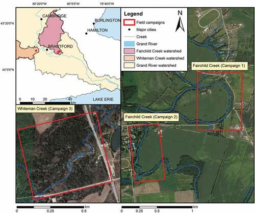
Fairchild Creek is a highly sinuous creek network that meets the Grand River south-east of the city of Brantford, draining an area of 401 km². The catchment of the creek is typical of southern Ontario being comprised of 66% cropland, 11% urban, 11% forest, and 13% wetland (Loomer and Cooke 2011). Fairchild Creek is of interest for conservation efforts as it contributes the highest amount of suspended sediments and phosphorus per km² to the Grand River (Lake Erie Source Protection Region Technical Team 2008). Study sites were chosen to be in the southern portion of the watershed where the creek flows through an agricultural setting. Both the banks and bed of Fairchild Creek are almost exclusively comprised of moderately stiff clays. Streambanks range in height from 1 to 4 m across the study extent with highly variable slopes.

Similar in catchment area to Fairchild Creek, Whiteman Creek flows into the Grand River west of Brantford and drains an area of 403 km². Whiteman Creek is located in an agricultural setting, with its land use composed of 76% cropland, 5% urban, 4% forest, and 16% wetland (Loomer and Cooke 2011). The study site chosen for Whiteman Creek flows through a heavily forested corridor and is located in the south-east portion of the watershed close to the creek’s outlet. The creek flows through the Norfolk Sand Plain as it approaches its outlet to the Grand River. The sand plain has high infiltration rates and much lower rates of surface runoff than the Haldimand Clay Plain where the Fairchild study sites are located (Loomer and Cooke 2011). The Whiteman Creek study site has a cobble bed and banks comprised of aggregates and sandy clays at the B and C horizons, and rich silts at the A horizon. Whiteman Creek has banks of 0.5–1.5 m in height, with undercutting and slumping visible, and gently sloping banks with thick riparian vegetation.

For each study site, streambank topography measurements were collected near-simultaneously using a TLS, UAV, and manual transect measurements; with an RTK-GNSS survey capturing all ground control points (GCPs). Field campaigns 1 to 3 respectively were conducted on 27 November 2028, and December 1 of 2017, with a preliminary campaign on November 22 used to review data collection methods and ensure protocols were upheld. Dates were chosen during the leaf-off period and when flow levels were below average to ensure safety for wading.

2.2. Terrestrial laser scanning (TLS) survey

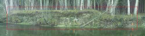
The TLS survey was conducted using a Leica Multistation MS50, Leica Viva GS14 and Leica Viva CS15 Field controller. The multistation can capture 1000 points per second up to 300 m away with mm level precision, which represents a distance measurement accuracy of 2 mm ± 2 ppm to any surface (Grimm 2013). While different surfaces and lighting conditions affect the accuracy of a TLS survey (e.g. Voegtle, Schwab, and Landes 2008), potential errors are still in the order of mm. A total of 23 scan locations were used to capture transects and the surrounding bank across the three field campaigns. A panoramic photo was taken with each scan to assign the pointcloud RGB values (see Figure 2). Scan distances were 15–25 m away from the bank of interest. For each TLS relocation a resection was performed using three GNSS points. GNSS points were recorded with the Leica Viva GS14 and Leica Viva CS15 Field controller using SmartNet’s GNSS network RTK. A total of 5,822,563 elevation points were collected capturing 760 m of bank face across the three campaigns (Table 1).

Table 1. Accuracy and image acquisition details of the TLS survey.

	Campaign 1	Campaign 2	Campaign 3
Location	Fairchild Creek	Fairchild Creek	Whiteman Creek
Length of bank (m)	223	246	291
Average GSD (m)	0.028	0.026	0.023
Point count	1,634,153	2,176,316	2,012,274
Vertical accuracy (m)	0.008	0.010	0.009
Horizontal accuracy (m)	0.010	0.013	0.011

Figure 2. A panoramic photo taken along Whiteman Creek with the Leica Multistation MS50. The red outline indicates the extent of the scanned streambank. The orange stakes on the streambank were used as ground control points for the UAV survey and for manual transect measurements. Additional stakes were placed closer to the stream to aid in manual measurements.

2.3. Unmanned aerial vehicle (UAV) survey

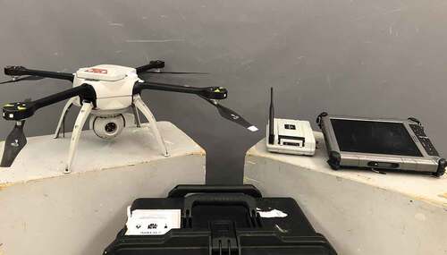
For this study, an Aeryon Labs Skyranger UAV was used for image acquisition (see Figure 3). The Skyranger is a vertical take-off and landing multi-rotor system with autonomous capabilities. Pre-programmed flight paths can be used for image acquisition via Aeryon Lab’s Mission Control Software with total flight times of up to 50 minutes. This UAV platform is compliant with federal regulations stipulated by Transport Canada. It is a versatile system that can be used in a wide range of environmental conditions including temperatures of −30–50°C, altitudes up to 1500 feet (457 m) above ground level (AGL), under 65 km hour^–1 sustained wind speeds, and has a maximum flight range of 3 km. The UAV was equipped with the SR-3SHD payload for image acquisition, which collects 15 megapixel RGB 4608 × 3288 pixel images. The payload has a 6.45 × 4.60 mm electro-optical sensor, aspherical lens, F/2.8, 7.5 mm focal length, rolling shutter, and a 46° field-of-view. The UAV system equipped with the SR-3SHD payload weighs a total of 2.8 kg.

Figure 3. Aeryon Labs Skyranger UAV system equipped with the SR-3SHD payload (left), base station and tablet (right).

Prior to each field campaign, a special flight operation certificate was obtained from Transport Canada, the local flight information centre was contacted to issue a Notice to Airmen (NOTAM) for flights at Whiteman Creek, and approval from NAV Canada was acquired. For each study site the UAV followed a preprogrammed flight path consisting of a 70% overlap (frontlap/sidelap) with nadir images acquired using a parallel-axis image acquisition scheme (see Figure 5 for Campaign 3). The UAV is equipped with a 3-axis gimbal to compensate for the pitch and roll of the UAV system. Despite large wind-gusts of 68 km hour^–1 and high sustained wind speeds (56 km hour^–1) during Campaign 2, the camera maintained a close to nadir orientation across all three campaigns with an average pitch of 3.11°, and an average roll of 2.14°. The flight height for the campaigns ranged from 40 to 50 m AGL which ensured tree canopy clearance, with an average ground-sampling-distance (GSD) of 0.023–0.028 m. For each field campaign, 14–16 wooden stakes were driven into the ground for use as GCPs. The top of each GCP was painted a fluorescent orange for aerial identification. Each stake was measured using RTK-GNSS and used to georeference the UAV imagery. A total of 89,586,885 elevation points were captured covering 4284 m of bank face across three campaigns (Table 2).

Table 2. Details for UAV campaigns and image acquisition.

	Campaign 1	Campaign 2	Campaign 3
Location	Fairchild Creek	Fairchild Creek	Whiteman Creek
Number of images	808	516	539
Area covered (m^2)	63,400	42,600	21,700
Length of bank (m)	2037	1281	966
Average GSD (m)	0.0086	0.0089	0.0082
Point count	47,847,307	23,797,741	17,941,837
GCPs	14	16	14

2.4. Southwestern ontario orthoimagery project (SWOOP)

In 2015 the Government of Ontario solicited a private contractor to acquire aerial imagery for southwestern Ontario, an area of 49,167 km². These image data are the result of private and government entities working together under the guidance of the Ontario Ministry of Natural Resources and Forestry (OMNRF). Flights were performed between April 12th and May 23rd between 2,506 and 2,535 m AGL using the ADS100 airborne digital sensor for imagery acquisition. An autocorrelated Digital Elevation Model (DEM) product was generated by an imagery contractor (Fugro) from the raw .las (.las is an industry standard file format for point data) vector elevation dataset for the purpose of ortho-rectifying the SWOOP 2015 orthophotography. The DEM was delivered to OMNRF as a derivative product as part of the imagery contract. A proprietary ‘steam rolling’ algorithm was used by the contractor to reduce raised surface features in the .las dataset. It is important to note that the DEM does not represent a full ‘bare-earth’ elevation surface. While the ‘steam-rolling’ algorithm has allowed for some raised features to be reduced closer to ‘bare-earth’ elevations (e.g. small buildings, small blocks of forest cover), many features are still raised above ground surface, such as larger buildings, larger forest stands and other raised features. Subsequently, a classified .las was generated by OMNRF Mapping and Geomatics Services Section (MGSS). MGSS staff worked with the raw point cloud .las data derived from image correlation in order to create a SWOOP 2015 classified .las. MGSS staff then derived a 2 m Digital Surface Model (DSM) and 2 m Digital Terrain Model from the 0.5 m classified pointcloud. These SWOOP derivatives are currently the only elevation dataset in southwestern Ontario with a sufficient spatial resolution for capturing streambank heights. The 0.5 m classified pointcloud data were included in our streambank surface model comparisons.

2.5. Manual transect survey

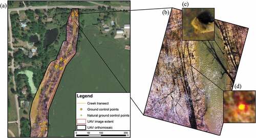
Manual surveying was done across 22 stream transects following the Ontario Stream Assessment Protocol (OSAP) which is a provincial standard recognized by the Ontario Ministry of Natural Resources and Forestry (Stanfield 2017). The point-transect sampling for channel structure methodology (i.e. Section 4: Module 2) was used for each transect. The wooden stakes used as GCPs from the UAV survey doubled as the transect locations for the manual survey (see Figure 4). Each stakes location was precisely recorded with RTK-GNSS. For each transect, two stakes were located on opposite sides of the creek from each other where overhead canopy cover was minimal and banks were traversable. A tape measure was pulled taut across each transect and fastened to the wooden stakes. A second tape measure was hung vertically from the first tape measure (i.e. transect line) and vertical measurements were recorded at 1 m intervals across the streambank profiles. Over the three campaigns, a total of 145 point-heights were captured on bank profiles. Additional manual measurements for stream characterization included a detailed vegetation inventory, soil bulk density, soil textural classification, and stream velocity measurements.

Figure 4. Study area for Campaign 2 illustrating: (a) the location of the manually measured creek transects, location of control points, and the UAV orthomosaic, (b) a single nadir UAV image (c) a ‘natural’ GCP (point captured on the edge of a fallen log), and (d) a GCP. TLS survey locations and bank accuracy assessments were conducted where control points were clustered.

2.6. Data processing

All data collected with the Leica Multistation MS50 were recorded in a proprietary data format only useable by Leica Infinity software, made by Leica Geosystems. Scanned pointclouds were initially loaded into Leica Infinity v.3.0.0.3068 to generate accuracy assessment reports (i.e. GNSS Coordinate Quality (CQ) values). The GNSS CQ values represent vertical (1D CQ) and horizontal (2D CQ) accuracies. Each point cloud was exported to a .las file format for use in CloudCompare v.2.9.1 (http://www.danielgm.net/cc/).

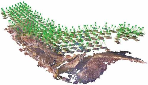
The UAV imagery was processed using the Pix4D v.3.2.10 (Pix4D SA, Switzerland) SfM-photogrammetry software application (see Figure 5 for Campaign 3). SfM software differs from other photogrammetry software applications in its ability to automate the process of 3D surface reconstructions with little to no manual input. A typical SfM workflow consists of the following four steps (Rumpler et al. 2014; Eltner et al. 2016), 1) keypoint generation and keypoint matching (i.e. finding homologous points between overlapping images), 2) iterative bundle adjustment to calculate a camera’s intrinsic and extrinsic properties and generation of a sparse pointcloud, 3) densification of the pointcloud, and 4) georeferencing with GCPs. The above workflow was followed for the SfM-pointcloud generation. Steps 1–3 involved processing of data collected over the three field campaigns in Pix4D comprising 1,907 images (5.73 GB) covering an area of 12.77 ha (127,700 m²) taken over six flights, which took approximately three hours of flight time. The data were processed on a Dell Precision Workstation 5810 Tower with Intel Xeon CPU E5-1620 v3 @ 3.5 GHz with quad-core, 8 processors, 64 GB RAM, operating Windows 7 64-bit and utilizing NVIDIA Quadro K4200 graphics card, which took 6 hours and 16 minutes for steps 1 to 3.

Figure 5. Pointcloud surface reconstruction of the Whiteman Creek stream corridor for Campaign 3. The pointcloud was derived using Pix4D with UAV imagery. Green spheres represent the optimized camera orientation and position where each image was taken. Flight lines were conducted with a 70% overlap at 40–50 m AGL. The reconstruction had a 57% success rate in recreating the streambank surface.

The most common workflow in the geosciences for camera calibration is the use of a self-calibrating bundle adjustment in Photoscan, Pix4D, or similar SfM software applications. We used a self-calibrating bundle adjustment in Pix4D for the initial pointcloud generation, using the default camera model of the SR-3SHD for an initial estimate on the camera’s intrinsic parameters (see Table 3), using a camera model with 5 distortions (i.e. three radial distortion terms, two tangential distortion terms). Other techniques for camera calibration include photographing a calibration pattern from different positions (e.g. Pérez, Agüera, and Carvajal 2013), two-step calibration with the distortions initially removed from all images (e.g. Gašparović and Gajski 2016), and a variety of camera pre-calibration techniques (e.g. Harwin, Lucieer, and Osborn 2015).

Table 3. Pix4D self-calibration results for the SR-3SHD camera. F is the focal length, P_x, P_y are the principal points (P_x, P_y is the image center), R₁, R_2, R₃ are three radial distortion coefficients, and T_1, T₂ are tangential distortion coefficients.

	F (mm)	Px (mm)	Py (mm)	R1	R2	R3	T1	T2
Pix4D Camera Model:	7.814	3.226	2.302	−0.115	0.072	−0.029	−0.003	−0.001
Optimized Camera Model:
Campaign 1	7.960	3.283	2.277	−0.127	0.107	0.014	−0.002	−0.001
Campaign 2	8.199	3.271	2.234	−0.131	0.142	−0.146	−0.002	−0.001
Campaign 3	8.201	3.276	2.333	−0.132	0.140	−0.085	−0.001	−0.001

GCPs were not incorporated into the bundle adjustment and georeferencing was conducted as a separate step (Step 4) using a 7-parameter 3D Helmert transformation. This transformation is a rigid linear transformation; using three rotations, three shifts, and one scaling factor to translate a pointcloud to a chosen coordinate system (Fonstad et al. 2013). The combination of one scaling factor used with a rigid and linear transformation ensures that relative distances and shapes will be maintained.

The pointclouds were split into a total of seven bank segments of interest for accuracy assessments. Each bank segment had six GCPs used for georeferencing. Several bank segments had GCPs obscured by overhead canopy, and ‘natural’ GCPs (i.e. natural features with a high contrast in the landscape) were using in lieu of them. A total of seven bank segments were chosen that were accurately recreated and overlapped with the TLS dataset: two from Campaign 1, two from Campaign 2, and three from Campaign 3. The seven chosen bank segments appeared to be stable due to thick riparian vegetation and cohesive clay soils.

For accurate comparison between all methods, the TLS, UAV, and SWOOP pointcloud data were filtered to generate bare-earth streambank surface models. All points not representative of the bank surface (e.g. farm fields, erroneous water returns, and vegetation) were manually filtered. To ensure the filtering process was comprehensive, the TLS and UAV pointclouds were then up-sampled to a 0.05 m resolution using the lowest return values to remove any remaining vegetation returns. The SWOOP dataset was down-sampled to the same 0.05 m resolution for comparison across the same number of points. All the datasets were georeferenced in the UTM zone 17N coordinate system.

2.7. Data analysis

We compared the accuracy of the streambank surface model derived from UAV SfM and a traditional photogrammetry dataset (i.e. SWOOP) to the benchmark of the TLS. While no formal benchmark exists for evaluating 3D surface reconstructions (except perhaps carefully measured RTK-GNSS points), the high accuracy and high point density of the TLS reduces potential error and is used as a benchmark for comparison of other 3D Surface reconstructions in erosional studies (e.g. Eltner et al. 2015; Smith and Vericat 2015; Prosdocimi et al. 2015). The TLS, UAV, and SWOOP datasets were kept in the .las file format and compared using cloud-to-cloud vertical distances; which is computed as the Euclidean distance between the nearest point-pairs (i.e. nearest neighbor distance) in CloudCompare. Every point had a corresponding point-pair for a distance calculation as each surface had the same grid size, with an average of 51,000 matching point-pairs per bank. A total of seven accuracy assessments were performed for the seven selected banks of interest. Manual measurements were compared to the TLS benchmark across 22 transects to assess vertical error.

3. Results

3.1. Streambank surface model accuracy

All the streambank surface models derived from the UAV, TLS, and SWOOP datasets were evaluated after the data were filtered and processed. The TLS survey produced accurate data across all the three field campaigns (see Table 4 for site information) with no visually discernable error. TLS location error from each resection using the GNSS points was very low (i.e. 0.01–0.03 m) across all three campaigns. Several scans had a low number of ground returns due to thick riparian vegetation but still generated sufficient coverage for comparison. For the purposes of using the TLS as a benchmark, the only error source for the TLS surface reconstruction was assumed to be the GNSS point inaccuracy.

Table 4. General site characteristics for each of the seven bank segments as calculated from the TLS. Banks 1–2 were captured in Campaign 1, Banks 3–4 were captured in Campaign 2, Banks 5–7 were captured in Campaign 3.

	Bank 1	Bank 2	Bank 3	Bank 4	Bank 5	Bank 6	Bank 7
Mean bank height (m)	3.5	1.3	2.0	1.9	0.6	1.8	0.7
Mean bank slope (°)	21.6	16.0	23.7	18.5	19.6	20.3	10.0
Wetted width (m)	16.9	14.5	11.8	11.8	16.4	16.4	13.2

Accuracy metrics (i.e. mean error, standard deviation [SD] of error, and root-mean-square-error [RMSE]) were generated for each technique and reported in Table 5 for each of the seven bank segments. Overall accuracy metrics for all three campaigns are summarized in Figures 6 and 8.

Table 5. Accuracy metrics (m) for seven bank segments. Banks 1–2 were captured in Campaign 1, Banks 3–4 were captured in Campaign 2, Banks 5–7 were captured in Campaign 3.

	Bank 1	Bank 2	Bank 3	Bank 4	Bank 5	Bank 6	Bank 7
UAV average error	−0.079	0.005	−0.001	−0.035	−0.012	−0.016	−0.073
UAV SD of error	0.193	0.056	0.071	0.082	0.049	0.110	0.117
UAV RMSE	0.209	0.056	0.071	0.089	0.051	0.111	0.138
SWOOP average error	0.001	−0.104	−0.024	0.055	−0.004	−0.140	0.081
SWOOP SD of error	0.249	0.254	0.238	0.192	0.181	0.316	0.157
SWOOP RMSE	0.249	0.275	0.239	0.200	0.181	0.345	0.176

Figure 6. Distribution of errors from UAV measurements relative to TLS measurements for a bank segment from each field campaign: (a) Bank 1 from Campaign 1, (b) Bank 3 from Campaign 2, (c) Bank 5 from Campaign 3, and (d) all seven bank segments (right; skewness −1.60, kurtosis 8.24). For each bank the mean error is negative, illustrating that UAV measurements over measured bank heights. Transformation error from georeferencing with GCPs was: RMSE (m) Bank 1: 0.175, Bank 3: 0.060, Bank 5: 0.038, overall average: 0.070.

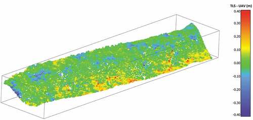
UAV measurements were the most accurate with respect to the TLS benchmark, but were still subject to a high variability in accuracy (Figure 6). The UAV pointcloud tended to over measure streambank elevation values, with a mean error of −0.030 m and a standard deviation of error of 0.097 m. This over measurement is expected due to the UAV nadir imagery capturing riparian vegetation and missing surface returns. Figure 7 shows the cloud-to-cloud accuracy assessment for a bank captured during Campaign 2 (Bank 3) showing the variation in streambank surface elevation values.

Figure 7. Bank 3 cloud-to-cloud elevation comparison in CloudCompare between the UAV streambank surface model and the TLS benchmark on a 20m segment of streambank.

The SWOOP pointcloud when compared to the TLS benchmark had a tendency to over predict elevation values similar to the UAV (Figure 8). The SWOOP had a mean error of −0.019 m with a standard deviation of error of 0.227 m. Additional comparisons were made to the SWOOP DSM, but the SWOOP DSM was found to be less accurate then using the pointcloud (mean error of 0.010 m with a standard deviation of error of 0.332 m across the seven bank segments) and was subsequently not used for any further analysis. The accuracy metrics of SWOOP presented here are not necessarily indicative of its actual accuracy. The study sites streambanks may have receded between 2015 and 2017 and subsequently changed surface elevation values. However, no visual pattern of bank erosion was present in any of the SWOOP streambank surface reconstructions; the error visually appeared to be randomly distributed across the bank profile and was not higher at the bank toe. This would suggest that both erosion and deposition were minimal for the chosen seven streambanks during this period.

Figure 8. Distribution of errors from SWOOP measurements relative to TLS measurements for a bank segment from each field campaign: (a) Bank 1 from Campaign 1, (b) Bank 3 from Campaign 2, (c) Bank 5 from Campaign 3, and (d) all seven bank segments (right; skewness −0.52, kurtosis 4.02). For each bank the mean error is negative, illustrating that SWOOP measurements over measured bank heights.

Manual measurements, made using the Ontario stream assessment protocol (OSAP), compared against the TLS benchmark had a systematic under measurement of streambank heights; 134 of the 145 point-heights were under measured when compared to the TLS benchmark across 22 transects. The manual measurements had a mean error of 0.238 m with a standard deviation of error of 0.195 m. Error in the range of ± 0.10 m was expected based on the field techniques for OSAP, however our measurements showed much higher error.

On average, manual transect measurements under measured elevation while both UAV and SWOOP surface models tended to over measure streambank elevation. The three datasets were benchmarked against TLS observations and attained an average RMSE of: UAV 0.104 m, SWOOP 0.238 m, and manual 0.274 m.

4. Discussion

The effects of streambank erosion on stream turbidity (e.g. Henley et al. 2000), temperature (e.g. Ryan 1991), and light attenuation (e.g. Kirk 1985; Hellström 1991), have significant impacts on water quality and the quality of marine habitat. Streambank surface models are an essential part of change-over-time analyses for measuring the magnitude of sediments being eroded from streambanks. The presented research takes a step towards understanding the accuracy of streambank surface models created with UAV SfM-based and traditional 3D reconstructions with respect to a TLS benchmark.

The presented data collection approaches vary in their feasibility for scaling out to large spatial extents (e.g. complete reaches, tributaries, or to the scale of an entire watershed). During a 6-hour field campaign, the TLS was able to capture between 223 and 291 m of bank face. Scan times averaged about 30 minutes per station relocation (with 6–7 relocations per campaign). In contrast, the UAV, during a full one-hour flight, was able to capture 6.34 ha of land area, which included a substantial amount of adjacent non-stream-corridor land, but corresponded to 2037 m of bank face (i.e. Campaign 1) with an average 52% success rate in recreating the streambank surface. Canopy cover and thick vegetation obscured the streambank from the nadir perspective for a portion of each field campaign leading to some incomplete streambank reconstructions. However, given six hours of flight time, the UAV would be able to map substantially more stream corridor than the TLS benchmark.

Our UAV imagery generated a sub-cm spatial resolution surface model that was finer than the spatial resolution of the TLS data. Although 3D surface reconstructions with TLS datasets are relatively straightforward, generating accurate surface reconstructions with UAV aerial imagery can be difficult. Error can be influenced by many factors including: lighting conditions, surface textures, GCP accuracy and quantity, image configuration (i.e. overlap, number of images, angle of view), and incorrect camera settings (Eltner et al. 2016).

Our initial data processing showed a doming effect (i.e. high error propagation towards the surface edge) in our streambank surface reconstruction. A parallel-axis nadir image acquisition scheme, which we used in our UAV survey, can cause the resultant pointcloud to contain artificial doming due to error accumulation in the SfM process (James and Robson 2014). This is due to an incorrect estimate of the camera model (i.e. radial distortion terms) being generated from the self-calibrating BA. Large variations in the estimations of our camera’s intrinsic parameters between campaigns (most notably the last radial distortion term; see Table 3) could be indicative of a poorly modelled camera. While this non-linear doming error was prominent on each campaign’s 3D reconstruction, our individually georeferenced streambanks used in the accuracy assessment exhibited only a small degree of this residual error; which can be seen from the georeferencing error. GCP RMSE from the Helmert transformation averaged 0.070 m for all seven bank faces. Georeferencing error was the highest on the longest bank measured (i.e. 65 m long Bank 1 – GCP RMSE of 0.175 m). The higher error was a function of residual doming error due to the length of the bank and a poor GCP network for georeferencing. Multiple ‘natural’ GCPs had to be used in lieu of our GCPs since they were obscured by canopy cover. Incorporating GCPs into the bundle adjustment in Pix4D would likely have mitigated some of this non-linear doming error. Additionally, using large flat GCPs (instead of vertical stakes) would have also improved our ability to locate each control point more accurately. The use of stakes as control points is not recommended, due to their small cross section, making them easily obscured by canopy cover. However, given our GCP placement along vegetated bank faces, the use of square flat GCPs was not possible.

To further explore the causes of error, the georeferencing error along with site condition variables (percent vegetated on bank face and top, percent canopy cover, vegetation type, slope, and bank height) was linearly regressed against UAV RMSE from TLS observations. Regression results showed that georeferencing error had a greater effect on the overall error than site condition variables, explaining more than 50% (R-squared value of 0.52) of the variance observed errors between the UAV and TLS. None of the site condition variables were statistically significant. The remainder of the unaccounted variance is likely to reside in flight parameters (e.g. height, image overlap), imaging sensor parameters (e.g. angle of image acquisition), imaging sensor platforms, weather conditions (e.g. incident solar radiation and angle), errors in the TLS surface creation (e.g. from vegetation), or other factors not compared such as different SfM algorithm and parameters. Since georeferencing plays such a key part in the accuracy of UAV-derived surface models, it is highly recommended to: 1) ensure all GCPs have a sufficiently wide cross section for accurate identification in aerial imagery, 2) include GCPs in the bundle adjustment to combat surface doming when modelling large spatial extents (James and Robson 2014), and, 3) ensure all GCPs are measured accurately (e.g. using RTK-GNSS).

Despite the variance of error in the UAV SfM streambank surface models, our accuracy results in complex topography are promising and are in agreement with existing UAV literature. Our UAV streambank surface models had a mean error of −0.030 m, with a RMSE of 0.104 m. In the best case, our UAV surface reconstruction yielded an RMSE of 0.051 m (Bank 5) relative to the TLS surface. Similar studies benchmarking the accuracy of UAV-derived surface models to that of a TLS or RTK-GNSS survey in fluvial environments have seen decimeter level accuracy in their UAV surface models (Flener et al. 2013; Mancini et al. 2013; Hamshaw et al. 2017; Elsner et al. 2018). While cm level accuracy is possible with UAV-derived surface models in certain landscapes (e.g. agriculture; Eltner et al. 2015), fluvial environments are more difficult to model. Some authors note a high variance in accuracy (e.g. RMSE of 0.033 m to 0.698 m; Hamshaw et al. 2017) in UAV-derived bank profiles, with a pronounced decrease in accuracy under vegetation cover. Studies in fluvial environments with little to no vegetation typically yield more consistent accuracies (e.g. beach survey RMSE of 0.101 and 0.132 m; Elsner et al. 2018; point bar survey RMSE of 0.088 m and 0.152 m; Flener et al. 2013). Our results show a range in error (i.e. RMSE of 0.051 m to 0.209 m) similar to the above error metrics. While vegetation and canopy cover led to incomplete SfM streambank reconstructions, out variance in error was more strongly correlated with georeferencing error. It is postulated that both the TLS and UAV surface models failed to model the streambank surface under thick vegetation, leading to similar surface elevations; but subsequently leading to incorrect error metrics on the vegetated bank surface. The results presented in this paper and in literature indicate that UAV-derived surfaces can have variance in accuracy, but should be suitable for monitoring streambank erosion at the decimeter level.

The streambank surface models in the SWOOP pointcloud data had a mean error of −0.019 m with a standard deviation of error of 0.227 m. The accuracy of SWOOP is stated to be 0.5 m both horizontally and vertically. Our study, even in complex topography with vegetation, found a good agreement with this 0.5 m benchmark (maximum accuracy achieved of 0.176 m RMSE; Bank 7). When UAV image acquisition is not feasible, traditional digital photogrammetry datasets could provide a valuable alternative data source for streambank surface models. Although the SWOOP dataset is less accurate than the TLS or UAV-derived surface models, it covers a much greater spatial extent than the other two techniques. As such, the SWOOP dataset is a promising choice for monitoring watershed-scale streambank erosion on a long time step (e.g. every 5 years).

Manual transect measurements performed the poorest across all three campaigns with a mean error of 0.238 m with a standard deviation of error of 0.195 m. Since wetted widths of the stream corridors ranged from 10 to 20 m and opposing streambanks differed in heights, it was difficult to ensure a level and completely taut measuring tape spanning the stream profile. This led to a systematic under measurement of elevations. Additionally, manual approaches are very limited in their applicability for 3D surface reconstructions, as a significant amount of interpolation is needed. While useful, the OSAP is both conceptually and experientially prone to consistent underestimation of bank heights and caution should be taken when interpreting data collected using a manual approach.

Despite the promising results of UAV SfM streambank surface models when compared to the other techniques, the constraints to broad scale applications of UAV to stream corridor mapping are primarily policy based. There are significant startup costs for equipment and training (e.g. Special Flight Operations Certificates in Canada, and Federal Aviation Authority Part 107 permitting in the United States, among other national-to-local requirements). Furthermore, the acquisition of legal permits to fly beyond visual line of sight (BVLOS) are not regularly approved, it can be very challenging to acquire regulatory approval for flights in proximity to populated areas, which both present a limitation to the optimization of the UAV for data acquisition. However, even given these policy constraints, the benefits and performance of UAV suggest that they will be utilized more regularly for steam corridor mapping for streambank erosion studies.

5. Conclusions

In this paper, we compared the accuracy of three different techniques for mapping out streambank topography compared to a TLS benchmark. UAV data proved to be the most accurate across all campaigns when compared to a TLS benchmark with an RMSE of 0.104 m. Both the UAV and SWOOP streambank surface models had a slight tendency to over measure bank heights, with mean errors of −0.030 m and −0.019 m respectively; manual transects had a strong tendency to under measure bank heights, with a mean error of 0.238 m. Both photogrammetrically-derived aerial datasets had reasonable accuracies even when measuring complex streambank topography with riparian vegetation. Manual transects measurements were the least accurate with the highest standard deviation of error. It is recommended to use UAV SfM-photogrammetry coupled with high accuracy GCPs for streambank topography mapping for erosional studies. TLS should be utilized for streambank erosion studies only at smaller spatial extents (e.g. less than 300 m of stream corridor). Future research should be aimed at optimizing flight plans for low-altitude UAV image acquisitions to better capture streambank topography which should seek to mitigate error propagation (i.e. doming) in SfM-photogrammetry, increase spatial coverage by supplementing nadir imagery with oblique imagery to generate surface models under canopy cover, as well as optimize flight parameters for accurate streambank mapping.

Acknowledgments

We would like to acknowledge with gratitude the funding provided by the Canadian Foundation for Innovation (32247), the Ontario Research Fund, and Aeryon Labs for equipment funding as well as the Ministry for Research and Innovation for an Early Researcher Award (ER15-11-198), and the Grand River Conservation Authority (GRCA) for student funding and other project costs. In addition, we would also like to thank Sandra Cooke, Bryan McIntosh, and the GRCA for their assistance with the project; Frank Kenny, Craig Onafrychuk, and the Ministry of Natural Resources and Forestry for providing assistance with SWOOP data; Omar Dzinic for assisting with fieldwork; and Sal Spitale and North South Environmental for conducting manual fieldwork measurements.

Disclosure statement

No potential conflict of interest was reported by the authors.

Additional information

Funding

This work was supported by the Early Researcher Award [ER15-11-198]; Aeryon Labs; Ontario Research Fund; Canadian Foundation for Innovation [32247]; Grand River Conservation Authority.

References

- Bernhardt, E. S., M. A. Palmer, J. D. Allan, G. Alexander, K. Barnas, S. Brooks, J. Carr, et al. 2005. “Synthesizing U.S. River Restoration Efforts.” Science 308 (5722): 636–637. doi:10.1126/science.1109769.
- Bilotta, G. S., and R. E. Brazier. 2008. “”Understanding the Influence of Suspended Solids on Water Quality and Aquatic Biota.”.” Water Research 42 (12): 2849–2861. doi:10.1016/j.watres.2008.03.018.
- Bull, L. J. 1997. “Magnitude and Variation in the Contribution of Bank Erosion to the Suspended Sediment Load of the River Severn, UK.” Earth Surface Processes and Landforms: the Journal of the British Geomorphological Group 22 (12): 1109–1123. doi:10.1002/(SICI)1096-9837(199712)22:12<1109::AID-ESP810>3.0.CO;2-O.
- Dietrich, J. T. 2016. “Riverscape Mapping with Helicopter-Based Structure-from-Motion Photogrammetry.” Geomorphology 252: 144–157. doi:10.1016/j.geomorph.2015.05.008.
- Elsner, P., U. Dornbusch, I. Thomas, D. Amos, J. Bovington, and D. Horn. 2018. “Coincident Beach Surveys Using UAS, Vehicle Mounted and Airborne Laser Scanner: Point Cloud Inter-Comparison and Effects of Surface Type Heterogeneity on Elevation Accuracies.” Remote Sensing of Environment 208: 15–26. doi:10.1016/j.rse.2018.02.008.
- Eltner, A., A. Kaiser, C. Castillo, G. Rock, F. Neugirg, and A. Abellán. 2016. “Image-Based Surface Reconstruction in Geomorphometry – Merits, Limits and Developments.” Earth Surface Dynamics 4 (2): 359–389. doi:10.5194/esurf-4-359-2016.
- Eltner, A., P. Baumgart, H. Maas, and D. Faust. 2015. “Multi‐Temporal UAV Data for Automatic Measurement of Rill and Interrill Erosion on Loess Soil.” Earth Surface Processes and Landforms 40 (6): 741–755. doi:10.1002/esp.3673.
- Flener, C., M. Vaaja, A. Jaakkola, A. Krooks, H. Kaartinen, A. Kukko, E. Kasvi, H. Hyyppä, J. Hyyppä, and P. Alho. 2013. “Seamless Mapping of River Channels at High Resolution Using Mobile LiDAR and UAV-photography.” Remote Sensing 5 (12): 6382–6407. doi:10.3390/rs5126382.
- Florsheim, J. L., J. F. Mount, and A. Chin. 2008. “Bank Erosion as a Desirable Attribute of Rivers.” AIBS Bulletin 58 (6): 519–529. doi:10.1641/B580608.
- Fonstad, M. A., J. T. Dietrich, B. C. Courville, J. L. Jensen, and P. E. Carbonneau. 2013. “Topographic Structure from Motion: A New Development in Photogrammetric Measurement.” Earth Surface Processes and Landforms 38 (4): 421–430. doi:10.1002/esp.3366.
- Gašparović, M., and D. Gajski. 2016. “Two-Step Camera Calibration Method Developed for Micro UAV’s.” International Archives of the Photogrammetry, Remote Sensing and Spatial Information Sciences XLI-B1 829–833. doi:10.5194/isprs-archives-XLI-B1-829-2016.
- González-Aguilera, D., J. Fernández-Hernández, J. Mancera-Taboada, P. Rodríguez-Gonzálvez, D. Hernández-López, B. Felipe-García, I. Gozalo-Sanz, and B. Arias-Perez. 2012. “3D Modelling and Accuracy Assessment of Granite Quarry Using Unmanned Aerial Vehicle.” ISPRS Annals of the Photogrammetry, Remote Sensing and Spatial Information Sciences I-3: 37–42. doi:10.5194/isprsannals-I-3-37-2012.
- Greig, S. M., D. A. Sear, and P. A. Carling. 2005. “The Impact of Fine Sediment Accumulation on the Survival of Incubating Salmon Progeny: Implications for Sediment Management.” Science of the Total Environment 344 (1–3): 241–258. doi:10.1016/j.scitotenv.2005.02.010.
- Grimm, D. E. 2013. “Leica Nova MS50: The World’s First Multistation.” GeoInformatics 16 (7): 22–26.
- Hamshaw, S. D., T. Bryce, D. M. Rizzo, J. O’Neil‐Dunne, J. Frolik, and M. M. Dewoolkar. 2017. “Quantifying Streambank Movement and Topography Using Unmanned Aircraft System Photogrammetry with Comparison to Terrestrial Laser Scanning.” River Research and Applications 33 (8): 1354–1367. doi:10.1002/rra.3183.
- Harwin, S., A. Lucieer, and J. Osborn. 2015. “The Impact of the Calibration Method on the Accuracy of Point Clouds Derived Using Unmanned Aerial Vehicle Multi-View Stereopsis.” Remote Sensing 7 (9): 11933–11953. doi:10.3390/rs70911933.
- Hellström, T. 1991. “The Effect of Resuspension on Algal Production in a Shallow Lake.” Hydrobiologia 213 (3): 183–190. doi:10.1007/BF00016421.
- Henley, W. F., M. A. Patterson, R. J. Neves, and A. D. Lemly. 2000. “Effects of Sedimentation and Turbidity on Lotic Food Webs: A Concise Review for Natural Resource Managers.” Reviews in Fisheries Science 8 (2): 125–139. doi:10.1080/10641260091129198.
- James, M. R., and S. Robson. 2014. “Mitigating Systematic Error in Topographic Models Derived from UAV and Ground‐Based Image Networks.” Earth Surface Processes and Landforms 39 (10): 1413–1420. doi:10.1002/esp.3609.
- Kirk, J. T. 1985. “Effects of Suspensoids (Turbidity) on Penetration of Solar Radiation in Aquatic Ecosystems.” Hydrobiologia 125 (1): 195–208. doi:10.1007/BF00045935.
- Kronvang, B., A. Laubel, and R. Grant. 1997. “Suspended Sediment and Particulate Phosphorus Transport and Delivery Pathways in an Arable Catchment, Gelbaek Stream, Denmark.” Hydrological Processes 11 (6): 627–642. doi:10.1002/(SICI)1099-1085(199705)11:6<627::AID-HYP481>3.0.CO;2-E.
- Lake Erie Source Protection Region Technical Team. 2008. Grand River Watershed Characterization Report. https://www.sourcewater.ca/en/source-protection-areas/resources/Documents/Grand/Grand_Reports_Characterization.pdf
- Laubel, A., B. Kronvang, A. B. Hald, and C. Jensen. 2003. “Hydromorphological and Biological Factors Influencing Sediment and Phosphorus Loss via Bank Erosion in Small Lowland Rural Streams in Denmark.” Hydrological Processes 17 (17): 3443–3463. doi:10.1002/(ISSN)1099-1085.
- Lawler, D. M. 1993. “The Measurement of River Bank Erosion and Lateral Channel Change: A Review.” Earth Surface Processes and Landforms 18 (9): 777–821. doi:10.1002/esp.3290180905.
- Longoni, L., M. Papini, D. Brambilla, L. Barazzetti, F. Roncoroni, M. Scaioni, and V. I. Ivanov. 2016. “Monitoring Riverbank Erosion in Mountain Catchments Using Terrestrial Laser Scanning.” Remote Sensing 8 (3): 241. doi:10.3390/rs8030241.
- Loomer, H. A., and S. E. Cooke. 2011. “Water quality in the Grand River Watershed: Current conditions & trends (2003 – 2008).” https://www.sourcewater.ca/en/source-protection-areas/resources/Documents/Grand/Grand_Reports_WaterQuality_2011.pdf
- Mancini, F., M. Dubbini, M. Gattelli, F. Stecchi, S. Fabbri, and G. Gabbianelli. 2013. “Using Unmanned Aerial Vehicles (UAV) for High-Resolution Reconstruction of Topography: The Structure from Motion Approach on Coastal Environments.” Remote Sensing 5 (12): 6880–6898. doi:10.3390/rs5126880.
- Niethammer, U., M. R. James, S. Rothmund, J. Travelletti, and M. Joswig. 2012. “UAV-based Remote Sensing of the Super-Sauze Landslide: Evaluation and Results.” Engineering Geology 128: 2–11. doi:10.1016/j.enggeo.2011.03.012.
- Osterkamp, W. R., P. Heilman, and L. J. Lane. 1998. “Economic Considerations of a Continental Sediment-Monitoring Program.” International Journal of Sediment Research 13 (4): 12–24.
- Pérez, M., F. Agüera, and F. Carvajal. 2013. “Low Cost Surveying Using an Unmanned Aerial Vehicle.” International Archives of the Photogrammetry, Remote Sensing and Spatial Information Sciences ISPRS Archive XL-1/W2. 311–315. doi:10.5194/isprsarchives-XL-1-W2-311-2013.
- Prosdocimi, M., S. Calligaro, G. Sofia, G. D. Fontana, and P. Tarolli. 2015. “Bank Erosion in Agricultural Drainage Networks: New Challenges from Structure‐From‐Motion Photogrammetry for Post‐Event Analysis.” Earth Surface Processes and Landforms 40 (14): 1891–1906. doi:10.1002/esp.3767.
- Quinn, J. M., R. J. Davies-Colley, C. W. Hickey, M. L. Vickers, and P. A. Ryan. 1992. “Effects of Clay Discharges on Streams.” Hydrobiologia 248 (3): 235–247. doi:10.1007/BF00006150.
- Resop, J. P., and W. C. Hession. 2010. “Terrestrial Laser Scanning for Monitoring Streambank Retreat: Comparison with Traditional Surveying Techniques.” Journal of Hydraulic Engineering 136 (10): 794–798. doi:10.1061/(ASCE)HY.1943-7900.0000233.
- Rosgen, D. L. 2001. “A Practical Method of Computing Streambank Erosion Rate.” Proceedings of the Seventh Federal Interagency Sedimentation Conference 1 (2): 18–26.
- Rumpler, M., S. Daftry, A. Tscharf, R. Prettenthaler, C. Hoppe, G. Mayer, and H. Bischof. 2014. “Automated End-To-End Workflow for Precise and Geo-Accurate Reconstructions Using Fiducial Markers.” ISPRS Annals of Photogrammetry, Remote Sensing and Spatial Information Sciences II-3: 135–142. doi:10.5194/isprsannals-II-3-135-2014.
- Ryan, P. A. 1991. “Environmental Effects of Sediment on New Zealand Streams: A Review.” New Zealand Journal of Marine and Freshwater Research 25 (2): 207–221. doi:10.1080/00288330.1991.9516472.
- Smith, M. W., and D. Vericat. 2015. “From Experimental Plots to Experimental Landscapes: Topography, Erosion and Deposition in Sub‐Humid Badlands from Structure‐From‐Motion Photogrammetry.” Earth Surface Processes and Landforms 40 (12): 1656–1671. doi:10.1002/esp.3747.
- Stanfield, L. 2017. Ontario Stream Assessment Protocol, Version 10. Peterborough, Ontario: Fish and Wildlife Branch, Ontario Ministry of Natural Resources. https://trca.ca/app/uploads/2018/02/osap-master-version-10-july1-accessibility-compliant.pdf
- Tamminga, A. D., B. C. Eaton, and C. H. Hugenholtz. 2015. “UAS‐based Remote Sensing of Fluvial Change following an Extreme Flood Event.” Earth Surface Processes and Landforms 40 (11): 1464–1476. doi:10.1002/esp.3728.
- Thoma, D. P., S. C. Gupta, M. E. Bauer, and C. E. Kirchoff. 2005. “Airborne Laser Scanning for Riverbank Erosion Assessment.” Remote Sensing of Environment 95 (4): 493–501. doi:10.1016/j.rse.2005.01.012.
- Triggs, B., P. F. McLauchlan, R. I. Hartley, and A. W. Fitzgibbon. 2000. “Bundle Adjustment – A Modern Synthesis.” Lectures Notes in Computer Science 1883: 298–372. Vision Algorithms: Theory and Practice. IWVA 1999. Springer: Berlin, Heidelberg. doi:10.1007/3-540-44480-7_21.
- Voegtle, T., I. Schwab, and T. Landes. 2008. “Influences of Different Materials on the Measurements of a Terrestrial Laser Scanner (TLS).” The International Archives of the Photogrammetry, Remote Sensing, and Spatial Information Sciences 37: 1061–1066.