A Sentinel-1 based hot-spot analysis: landslide mapping in north-western Italy

ABSTRACT

The 6-days repeatability of Sentinel-1 constellation allows building up an interferometric stack with unprecedented velocity. Easily updatable hot-spot analyses, frequently repeated following the update of Sentinel-1 images, represent very useful tools for MTInSAR (Multi-Temporal Interferometric Synthetic Aperture Radar) data analysis. Mountain regions are a challenging environment for interferometric analyses because of their climatic, morphological and land cover characteristics. In this context, MTInSAR data can retrieve reliable information over wide areas, with high cost-benefits ratio and where the installation of ground-based devices is not feasible. Considering the well-known limitations of interferometric techniques (such as fast motions or temporal and spatial decorrelation), hot-spot analyses are a viable solution for semi-automatic ground movements extraction over mountain regions. In this work, we present an example of a hot-spot analysis applied to a large stack of MTInSAR products generated by means of SqueeSAR technique over an alpine region (Valle d’Aosta, north-western Italy). The obtained outputs allow detecting 277 moving areas connected to landslides and mass wasting processes in general. These products are intended to be implemented in the landslide risk management chain of the region, focusing on landslide state of activity definition and landslide mapping.

1. Introduction

Mountain regions are particularly prone to mass wasting processes because of the high energy of the relief, strongly influenced by climate changes that create peculiar landscapes characterized by a strong disequilibrium of the slopes (Haeberli, Schaub, and Huggel 2017). Nowadays, the combination between climate, geological asset, glacial rebound, seismicity, slope geometry and weathering generates a wide range of slope instabilities: from flank-scale Large Deep-Seated Gravitational Slopes Deformations (DSGSD) to debris flows, complex landslides, rockslides and rockfalls.

Because of the orography of mountain environments, it is sometimes difficult to gather in situ deformation data. Satellite-based interferometric techniques try to overcome this limitation thanks to the possibility to obtain wide area coverage data with a great cost-benefits ratio compared to classical ground measurements (Singhroy 2009; Tomás et al. 2014). Multi-temporal Interferometric Synthetic Aperture Radar (MTInSAR) approaches have been widely used to map and monitor slope instabilities in mountain regions all around the world (Righini, Pancioli, and Casagli 2012; Herrera et al. 2013; Oliveira et al. 2015; Raspini et al. 2016; Bianchini et al. 2017; Imaizumi et al. 2018).

MTInSAR data demonstrated their usefulness not only for single landslide reconstruction and characterization (Calò et al. 2012; Bovenga et al. 2013; Necsoiu, McGinnis, and Hooper 2014; Del Soldato et al. 2018; Solari et al. 2018b), but also for landslide mapping and landslide inventory updating at regional scale (Notti et al. 2010; Meisina et al. 2013; Ciampalini et al. 2015; Di Martire et al. 2017; Rosi et al. 2018). These bibliographic examples show how MTInSAR products can be used as a proxy for ground motion detection over wide areas. The information collected in this way have begun to be acknowledged not only by the scientific community but also by regional and national authorities in charge of hydrogeological risk management and by Civil Protection entities. Considering Italy, satellite interferometric products are currently implemented in Civil Protection practices in the framework of regional and local hydrogeological emergencies (Pagliara et al. 2014; Raspini et al. 2017).

In this context, the launch in April 2014 of the first Sentinel-1 satellite opened new frontiers for radar images exploitation. In fact, the Sentinel-1 constellation has been designed by the European Space Agency (ESA) for specific scientific uses, relying on a regular acquisition plan with a worldwide coverage (Torres et al. 2012). The regional scale mapping capabilities of Sentinel-1 are guaranteed by the TOPSAR (Terrain Observation with Progressive Scans SAR) acquisition mode (De Zan and Guarnieri 2006) and by the policy of free and open access data for the final users of the radar images (Showstack 2014).

The Sentinel-1 constellation represents the natural evolution of previous ESA satellites (ERS 1–2, European Remote Sensing satellites, and Envisat) and operates in C-band with 6 days repeatability. The low temporal baseline between images allows building up long and frequently updated time series of deformation as well as to obtain a better ground response in terms of radar coherence (Plank 2014). The potentialities of Sentinel-1 radar images have already been successfully exploited by some authors to monitor landslides at both regional and local scales. Barra et al. (2016) presented one of the first application of Sentinel-1 radar images for landslide detection and mapping at a regional scale (Molise Region, Italy). Dai et al. (2016) monitored the Daguangbao mega-landslide combining high-resolution Digital Elevation Models (DEM) and Sentinel-1 interferometry. Béjar-Pizarro et al. (2017) presented a reproducible methodology to derive vulnerable buildings maps affected by slow-moving landslides starting from Sentinel-1 MTInSAR products. Fiaschi et al. (2017) tested the potentialities of Sentinel-1 MTInSAR data for landslide mapping in a municipality located in Northern Italy and characterized by densely vegetated areas. Intrieri et al. (2018) applied the Fukuzono method to Sentinel-1-derived time series of deformation for post-event estimation of the failure time of a large rock avalanche in the Sichuan Province (China). The presence of a clear pre-failure acceleration was confirmed by Dong et al. (2018) using a different MTInSAR approach. Raspini et al. (2018) showed the first worldwide application of a near-real-time monitoring system based on a systematic processing infrastructure of Sentinel-1 data at a regional scale. These works demonstrate how Sentinel-1 images can produce reliable results at different scales, producing frequently updated time series of deformation useful for the early detection of motion changes.

In this work, we exploited Sentinel-1 images for active motions mapping at regional scale. The test area is the Valle d’Aosta (VdA), a mountain region located in North-western Italy, at the border with France. The region is characterized by a wide variety of slope instabilities, encompassing DSGSD and complex or rotational landslides as well as rockfalls and debris flows. We propose a regional scale approach aimed at defining moving areas, mainly related to already known or not known landslides, starting from large datasets of Permanent Scatterers (PS) acquired in both orbits and generated by means of SqueeSAR algorithm. To our knowledge, this is the first example of Sentinel-1 data processing at the regional scale along the Alpine arc; thus, the results obtained represent a huge improvement for landslide knowledge in VdA. Sentinel-1 data are the starting point of a methodology aimed at rapidly highlighting all the moving areas above a certain velocity threshold, removing outliers and creating clusters of PS characterized by common deformation patterns. The methodology is designed to create a priority list of active motions to be used for Civil Protection and urban planning activities. Moreover, the products generated provide useful information for landslide activity mapping at regional scale.

2. Geographical and geomorphological context

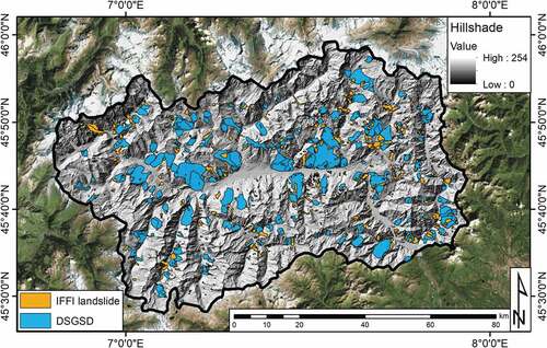
Valle d’Aosta (VdA) is the smallest Italian Region, covering only 3262 km². Almost 50% of its territory has an elevation higher than 2000 m a.s.l., thus it can be considered as a mountain region with peaks reaching 4000 m a.s.l. and main valleys above 300 m a.s.l. (Figure 1).

Figure 1. Geographical localization and hillshade model (derived from a 10 m DEM) of the Valle d’Aosta Region. The landslide contours and the DSGSD are included in the IFFI catalogue of VdA. The map is overlaid on a ESRI World Imagery map

Esri, DigitalGlobe, GeoEye, Earthstar Geographics, CNES-Airbus DS, USDA, USGS, AeroGRID, IGN, and the GIS User Community.

From the geological point of view, VdA is part of the Western Alps, cutting through the main alpine structural domains: Austroalpine, Penninic and Helvetic (Dal Piaz, Bistacchi, and Massironi 2003). All the units show a metamorphic imprinting passing from eclogitic or blueschist facies to low-grade metamorphism (Frey, Desmons, and Neubauer 1999). Therefore, the geological context of VdA is characterized by a complex pile of metamorphic-tectonic nappes, consequence of an intense post collisional and neo-tectonic activity (Bistacchi et al. 2001). Thus, the tectonic and geo-structural characters influenced the evolution of the reliefs and the current slope dynamics (Martinotti et al. 2011).

Glacial action is another main factor that controls the past and current orography of VdA (Martinotti et al. 2011). The main morphological traits of VdA are: a central valley, east–west orientated, in which the Dora Baltea River flows, and several lateral and tributaries valleys north–south orientated. This configuration is a remnant of the Quaternary glacial modelling that is still influencing slope dynamics (Carraro and Giardino 2004). The glacial morphology has been progressively deepened by fluvial action that eroded glacial landforms, depositing alluvial fans at valley bottoms (Martinotti et al. 2011).

VdA has a high population density only along the main valley whereas entire portions of the regional territory are partially or totally inhabited. The land cover is mainly composed of forests and grasslands, gradually replaced at high altitudes by exposed rocks, debris with sparse or no vegetation and glaciers. This environmental asset is strongly influenced by local climatic variations produced by high peaks that act as morphological barriers for humid air masses coming from the Mediterranean Sea or the Atlantic Ocean (Ratto, Bonetto, and Comoglio 2003). Thus, the morphology of VdA creates a wide spectrum of temperature and snow or rain precipitation regimes in which mountainous areas records abundant snowfalls and average rainfalls around 1000–1100 mm year^–1, whereas along the main valley the climate is drier with average precipitation around 600 mm year^–1 (Ratto, Bonetto, and Comoglio 2003).

In the VdA Region, 2052 landslides have been mapped in the framework of the Italian Landslide Inventory (IFFI) project, founded by the Italian Government and conducted by the Institute for Environmental Protection and Research (ISPRA) starting from 1999 (Trigila, Iadanza, and Spizzichino 2010). The VdA database includes both landslide and DSGSD phenomena, covering 592 km², and has been updated in 2015 (Figure 1). The landslide index (ratio between the area covered by landslides and the regional territory) of the region amounts to 18%. Thirty per cent of landslides mapped are classified as rockfalls (including topples) mainly affecting metamorphic rocks (Giardino and Ratto 2007). Shallow landslides and mud or debris flows are quite frequent as well, composing 24% of the landslides mapped. These landslides are related to intense rainfalls events that also locally induce flooding (Salvatici et al. 2018). Despite being only 13% of the total known phenomena, DSGSD cover 76% of the total area occupied by slope instabilities, sometimes involving entire mountain flanks (e.g. Hône, Villeneuve, Quart and Breuil-Cervinia DSGSD – Martinotti et al. 2011).

Considering its geomorphological and climatic context, VdA is characterized by mass movements related to periglacial landforms, such as rock glaciers, that are quite common in alpine environments (Haeberli et al. 2006). Rock glaciers are defined as ice-rich or frozen debris steadily creeping along non-glacierized mountain slopes; they are commonly subdivided inactive, inactive or relict, depending on their ice content (Haeberli et al. 2006). Active rock glaciers register a steady-state creep with deformation rates varying from cm year⁻¹ to several m year⁻¹ (Haeberli et al. 2006), whereas inactive and relict rock glaciers, because of the low or null ice content, do not almost move (Barsch 1996). In VdA 937 rock glaciers are mapped, covering 2% of its territory; 57% of them are classified as relict (Morra Di Cella et al. 2011). Active rock glaciers are usually found above 2200 m a.s.l. along north-exposed slopes, whereas relict landforms are found at lower altitudes, but never below 1600 m a.s.l. (Cignetti et al. 2016).

2.1. Radar visibility of the Valle d’Aosta region

Because of its climate, morphology and land cover, VdA is a challenging environment for interferometric analyses. It is possible to derive the theoretical distribution of the PS data knowing the acquisition geometry of Sentinel-1 and the topography of the area. For this aim, we exploited the methodology presented by Notti et al. (2014) that allows deriving the Corrected Range Index (CRI), a combination between the effects of topography (Range Index – RI) and land cover (Land Cover Index – LUI) on PS points detection. This approach, previously exploited by Cignetti et al. (2016) for ERS 1–2 and Envisat data in the same context, is useful to a-priori detect areas where PS detection is impossible or where, because of local slope orientation, PS measurement will underestimate the real ground motion.

The CRI is obtained as a weighted average of RI and LUI. The RI depends on the terrain morphology (slope and aspect) and on the radar geometry (incidence and azimuth angles). The LUI is derived from an empirical classification of land cover that depends on the land use, on the sensor band, as well as on the PSI processing (see Table 1 in the Supplementary Materials). The final output is a colour scale map that, as well as RI and LUI, is simply derived in a GIS (Geographic Information System) by means of standard tools, common for most of the GIS environments. For an explanation on how the indexes are calculated we refer to Chapter 1 of the Supplementary Materials.

The CRI results for the entire VdA Region show how the PS distribution will be strongly affected by both local morphology and land use. Depending on the orbit, eastward or westward valleys could be partially visible or in complete shadowing, this is especially evident along the tributaries valleys of the Dora Baltea (values below 20 in Figure 2). These ‘low PS density’ areas are represented by values of CRI below 20, covering around 25% of the total VdA territory. It is worth noting that along these valleys is quite rare to obtain shadowing zones in both orbits; the coverage of at least one orbit is most of the time guaranteed. Values of CRI near zero are also registered where LUI tends to zero, i.e. in areas with perennial ice coverage or in water basins. This is evident along the north-north-western border of the VdA where the largest ice sheets are present.

Figure 2. CRI maps for the Valle d’Aosta Region. (a) and (b) are referred to the ascending and descending orbits, respectively. The maps are overlaid on a ESRI World Imagery map

Esri, DigitalGlobe, GeoEye, Earthstar Geographics, CNES-Airbus DS, USDA, USGS, AeroGRID, IGN, and the GIS User Community.

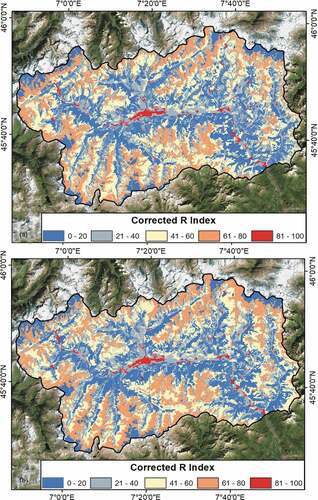
On the other hand, CRI values higher than 60 indicate a high to very high radar visibility. Twenty-two per cent of the regional territory records these values. Very high CRI values are recorded only along the flat Dora Baltea valley where the largest urban areas are present; here the density of PS measurements depends only on the type of surface. It is recalled that the CRI index depends only on the land use when the effect of the topography is low, i.e. when RI is above 50. High values of CRI are found along favourably orientated valleys, depending on the acquisition geometry, and at high altitudes, where the vegetation is sparse or absent and where debris or outcropping rocks dominate the landscape. Here, the PS density is in theory quite high, but the winter snow coverage reduces the coherence of the radar images, leading to a lower density of PS points with respect to the calculated value of CRI (Notti et al. 2014).

3. Methodology

The concept of the methodology is to extract moving areas from large interferometric datasets that are subsequently radar-interpreted by using simple GIS (Geographical Information System) tools (Farina, Casagli, and Ferretti 2007). The final output is a geo-database containing multiple information, regarding both magnitudes of ground motion and type of process that triggered it. In addition, a qualitative parameter for the evaluation of the ‘interferometric reliability’ of each moving area is derived. Following this concept, the methodology is subdivided into three main phases:

1. deformation map generation;

2. moving areas mapping;

3. radar-interpretation and geo-database compilation.

3.1. Deformation map generation

The methodology starts with the generation of a deformation map over the entire VdA region, producing one of the first examples of Sentinel-1 wide area products derived for the Alpine arc. The ground deformation map is derived by analysing two large stacks of C-band Sentinel-1 images by means of the SqueeSAR algorithm (Ferretti et al. 2011). This algorithm represents the evolution of PSInSAR, firstly developed in 2000 by Ferretti, Prati, and Rocca (2001).

The novelty of PSInSAR algorithm is the capability of identifying point-like-targets (Permanent Scatterers) within the radar image, such as pixels corresponding to man-made objects, outcropping rocks, debris areas or buildings that register a stable radar signal across the whole interferometric stack. The definition of these points allows reducing decorrelation phenomena and obtaining a high signal-to-noise ratio (Ferretti, Prati, and Rocca 2001). One limitation of this technique is the impossibility of identifying ‘radar friendly’ targets outside of urban and peri-urban areas and in highly vegetated zones.

SqueeSAR has been developed to partially overcome this limitation, estimating deformation rates not only from point-like-targets but also from partially coherent pixels, called Distributed Scatterers (DS). DS points correspond to homogeneous ground surfaces and not to single objects, i.e. uncultivated areas, deserts, debris covered slopes and scattered outcrops. The base idea of SqueeSAR is to select sets of Statistically Homogeneous Pixels (SHP) using a space adaptive filter (DespecKS, Ferretti et al. 2011) based on the Kolmogorov-Smirnov statistical test (Kvam and Vidakovic 2007). The test is run directly on the amplitude values of the pixels of the radar image, finding all the possible SHP within a search window (usually one hectare large, (Ferretti et al. 2011). All the pixels, with common radar characteristics within the search radius, are considered as a homogeneous population (thus being DS) and further analysed. At this point, the DespecKS filter is used to 1) reduce the speckle noise of each set of DS without changing the intensity and amplitude values of the point-like targets (i.e. PS) and 2) estimate the complex coherence matrix of every set of DS (Ferretti et al. 2011). The phase values of every DS coherence matrix are optimized exploiting the Phase Triangulation Algorithm (PTA – Ferretti et al. 2011). The result obtainable is a mixed selection of PS and DS that are jointly processed by means of the standard PSInSAR approach (Ferretti, Prati, and Rocca 2001).

In this work we exploited Sentinel-1A and 1B radar images acquired in C-band (wavelength equal to 5.55 cm) in ascending (tracks 88) and descending (track 66) orbits. Both data stacks are composed of 130 images reaching the end of February 2018, starting from October 2014 for the ascending orbit and from November 2014 for the descending orbit.

3.2. Moving areas mapping

Filtering regional-scale MTInSAR products is a fast way to identify the most potentially hazardous motions, obtaining a preliminary product that could be further analysed and on-field validated. In this work, we extracted moving areas using a simple and reproducible method, using a hot-spot-like approach already followed by other authors (Meisina et al. 2008; Bianchini et al. 2012, 2013; Barra et al. 2017).

Firstly, the deformation map is filtered to extract the PS points in both orbits that records the highest deformation rates above the region. A stability threshold equal to 10 mm year^–1 is set to this aim. This quite high value, equal to 5 times the standard deviation of the datasets, has been chosen for detecting only the highest deformation rates that commonly characterize unstable rock debris on the steep slopes of VdA. The value is near the 16 mm year^–1 threshold used by Cruden and Varnes (1996) for distinguishing very slow and slow landslides. Moreover, this value has been chosen jointly with the regional authorities, considering their specific requirements. Considering this, we will not map DSGSD-related deformation that involves large slope sectors with deformation rates frequently lower than 10 mm year^–1 (Crosta, Frattini, and Agliardi 2013). Activations of portions of DSGSD systems are anyway a priori not excluded.

Secondly, the filtered deformation maps are further analysed to extract significant deformation clusters and remove isolated, non-representative, points. This is done by buffering the PS points of the filtered deformation maps and then automatically join the adjacent PS in a GIS environment. We choose a buffer size of 100 m and a minimum cluster size of three PS points for obtaining the final moving areas. There is not a standard law to define the buffer size and the minimum number of PS within each cluster; they are selected on the basis of the previous knowledge of an area and on landslide type and size (Bianchini et al. 2012). In general, a small buffer size prevents the identification of clusters where the PS density is low (as in mountain areas). The minimum cluster size defines how much small groups of PS are representative for the phenomena to be monitored.

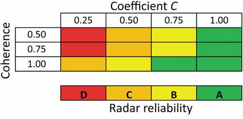
Finally, for each moving area, an index of the ‘interferometric reliability’ of the measured deformation is derived. This index is based on two parameters: i) mean coherence of the time series of the PS points composing the cluster and ii) percentage of the real ground motion vector that can be registered considering the Line Of Sight (LOS) of the sensor (coefficient C). Coherence is used as a proxy for the noise of the time series, considering the parameter as the deviation between the linear model used to calculate the velocity and the real-time series. This parameter gives hints on the presence of possible non-linear deformation affecting the PS point. Coefficient C is calculated starting from a relationship between slope, aspect and direction cosine of the LOS, as defined by Notti et al. (2014). This parameter is a powerful index for evaluating the magnitude of the real displacement vector that can be seen along the LOS of the sensor. A 30 m resolution SRTM (Shuttle Radar Topographic Mission) provided by NASA (National Aeronautics and Space Administration) was used to calculate the C index; this is required for smothering the topography, considering that the index is quite sensitive to small slope variations (in terms of orientation). The index has been designed for landslide studies; thus, low angle slopes (below 5°) and flat areas are not considered in its calculation. Coefficient C ranges between −1 and 1; values close to zero means that the ground motion cannot be correctly estimated or that can be highly underestimated.

For combing coherence and C index we defined a contingency matrix, shown in Figure 3. The result of the matrix is a code that expresses the level of interferometric reliability depending on the quality of the time series (coherence) and on the topography effect (coefficient C). The final moving areas are delivered in shapefile format, one for each orbit, containing the value of mean velocity, mean coherence, mean standard deviation and interferometric reliability of each one of them.

Figure 3. Contingency matrix for the calculation of the interferometric reliability of each moving area. Values ranges between D (not reliable) and A (high reliability)

3.3. Radar-interpretation and geo-database creation

To provide a complete database of ground motions, functional for Civil Protection practices, the moving areas have to be radar interpreted and included into a specifically designed geodatabase.

In addition to the interferometric data, the geodatabase contains information regarding:

• geographical localization of the moving area, i.e. municipality, local toponym, nearest road name;

• morphological context, i.e. mean altitude and slope;

• intersection between moving areas and VdA landslide inventory (i.e. 2015 IFFI catalogue). If a moving area contains or is contained into an already mapped landslide specific information regarding the phenomenon will be added to the geodatabase (type of movement, identification code, year of occurrence and so on);

• intersection between moving areas and VdA catalogue of rock glaciers. These data could be useful to identify high-altitude instabilities related to permafrost-rich rock masses. The catalogue is available online and contains information about the location of glaciers and rock glaciers and their state of activity (Valle d’Aosta Region Glaciers and Rock Glaciers Catalogue. http://catastoghiacciai. regione.vda.it/Ghiacciai/Main Ghiacciai.html# – Accessed on 10 September 2018).

4. Results

Following the schema of the methodology, the results obtained in each phase will be presented. In addition, some examples of active deformation will be proposed.

4.1. Deformation maps

Despite the challenging environment, the SqueeSAR processing of Sentinel-1 images gives good results in terms of both densities of points and noise of single measurements. Considering the high number of images composing the Sentinel-1 datasets, the estimation of the displacements rates easily reaches a precision higher than 1 mm year^–1 (Raspini et al. 2018). The outputs of the interferometric investigation are shown in Figure 4. Almost 360,000 points for each orbit were found, obtaining a mean density of around 100 PS kilometre⁻². The density is maximum along the Dora Baltea valley, in correspondence of the city of Aosta, whereas it is minimum along tributaries valleys where shadowing and layover effects are possible (values below 20 in Figure 3). No PS are registered where high vegetation or the presence of ice strongly limited the coherence of the radar images, as predicted by the CRI (Figure 3).

Figure 4. Deformation maps, derived using the SqueeSAR algorithm, for the VdA Region. (a) ascending orbit results, (b) descending orbit results. 1) Punta Chaligne DSGSD; 2) Torgnon DSGSD; 3) Cervinia DSGSD; 4) Emarese DSGSD; 5) Valgrisenche Valley; 6) Cogne Valley; 7) Rhêmes Valley; 8) Valsavarenche Valley. The maps are overlaid on a ESRI World Imagery map

Esri, DigitalGlobe, GeoEye, Earthstar Geographics, CNES-Airbus DS, USDA, USGS, AeroGRID, IGN, and the GIS User Community.

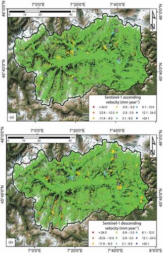
Considering a threshold of 3 mm year^–1, equal to 1.5 times the standard deviation of the estimated velocity values of the datasets, 94.4% of the PS in ascending orbit and 92.9% in descending orbit are considered as stable (Figure 4). This fact means either that the PS points do not record any ground motion or that the deformation rate is so small that it cannot be distinguished from the noise without a detailed analysis.

Significant clusters of moving points outside the 3 mm year^–1 threshold have been anyway registered, sometimes involving entire slope sectors. It is interesting to notice that in some cases the terrain morphology allows obtaining consistent results in both orbits. This is evident considering some well-known large slope deformations such as the Punta Chaligne, Torgnon, Cervinia and Emarese DSGSDs (areas 1 to 4 in Figure 4(a,b)). All these large slope phenomena records velocities outside the stability threshold, ranging between 5 and 10 mm year^–1, as expected for this type of movements (Crosta, Frattini, and Agliardi 2013).

The effects of slope aspect can be seen by the results obtained along N-S orientated valleys in the south-western portion of VdA. Along these valleys deformation rates above the stability threshold, up to 20–30 mm year^–1, are usually recorded in one single orbit. This is the case of the left flanks of Valgrisenche and Cogne Valleys in ascending orbit (points 5 and 6 in Figure 4(a)) and of the right sides of Rhêmes and Valsavarenche Valleys (points 7 and 8 in Figure 4(b)).

4.2. Moving areas mapping

The methodology explained in Section 3.3 allows extracting a total of 277 moving areas in the test site (Figure 5), 115 for ascending orbit, with mean velocity values ranging from −39 mm year^–1 to 33 mm year^–1, and 152 for descending orbit (the mean velocity range is equal to −60 mm year^–1 – +18 mm year^–1). Moving areas are composed by a minimum of 3 PS points, as required by the methodology, and a maximum of 123 and 207 PS in ascending and descending orbit, respectively. On average, moving areas contain 10 PS points in ascending orbit and 18 PS points in descending orbit.

Figure 5. Moving areas above the 10 mm year^–1 threshold. The black contours represent the borders of VdA municipalities. The hillshade is derived from a 10 m resolution DEM of VdA. 1) Bosmatto landslide; 2) Allesaz landslide; 3) Ayas municipality; 4) Saint Rhémy En Bosses municipality. The data are overlaid on a ESRI World Imagery map

Esri, DigitalGlobe, GeoEye, Earthstar Geographics, CNES-Airbus DS, USDA, USGS, AeroGRID, IGN, and the GIS User Community.

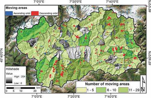
Moving areas are quite widespread in VdA, with two maximum density sectors along Rhêmes and Cogne valleys (see Figure 4(a,b) for the localization). Seventy-one per cent of VdA municipalities host at least one moving area; 27% of them records more than five deformation clusters and only 9% more than 15 (Figure 5). Thirty-two per cent of the municipalities registered the presence of only one moving area. The maximum number of moving areas (28) are found within the Ayas municipality, located in the north-eastern part of the region (polygon enclosing point 3 of Figure 5).

Considering the radar reliability of the moving areas, 40% and 46% of the areas in ascending and descending orbits, respectively, are considered as ‘highly reliable’ (grade A of the contingency matrix of Figure 2). This means that both the time series and the measurement of displacement vector are representative of the real movement along the slope. On the other hand, 6% (ascending orbit) and 15% (descending orbit) of the clusters obtain a D grade (Figure 2), meaning that the PS time series are noisy or follow a non-linear trend and, because of the terrain morphology, the real displacement vector is strongly underestimated. The percentage for the ascending orbit is the result of a higher weight of the local morphology, with some clusters detected along southward or northward slopes.

The spatial overlapping between moving areas of different orbits is not quite common. This is due to slope orientation effects, i.e. velocity variations in the same area considering different orbits and shadowing effects, i.e. impossibility of obtaining data because of the presence of steep morphologies that prevent the identification of PS in one of the two orbits.

Landslides and slope mass wasting phenomena are the main target of this work. Thus, we overlapped the IFFI catalogue with the database of moving areas in both orbits. Twenty-eight per cent and 38% of the moving areas in ascending and descending orbits, respectively, fall into the contours of already known landslides. Almost half of the moving areas are found in the correspondence of debris deposits along steep slopes connected to the recent activity of rock falls. The largest part of these motions is found at high altitude, preferentially above 2000 m a.s.l. Complex and rotational landslides equally represent the remaining 50% of the landslides. Some of these active deformations are part of large DSGSD; however, they indicate a localized motion not related to an entire flank-scale movement. We found that 25% of all the moving areas fall into the perimeter of a known DSGSD.

Ten per cent of the moving areas in ascending orbit (12 in total) fall within the perimeter of a mapped rock glacier, 6 classified as active and 6 as relict. In descending orbit, the percentage reaches the 15% (24 moving areas), subdivided into 18 active rock glaciers and 6 relicts. Because of the presence or not of an active permafrost layer, mean velocity values differ between the two types of rock glaciers. Relict forms are barely above the 10 mm year^–1 threshold, whereas active rock glaciers reach values three times higher. This difference has been already highlighted by Cignetti et al. (2016) using ERS 1–2 and Envisat interferometric products.

Figure 6 presents two examples, taken from two valleys located in the north-eastern part of VdA, of moving areas falling within the perimeter of already mapped landslides (IFFI catalogue). The first moving area is affected a well-known landslide located above the village of Bosmatto in the Gressoney Saint Jean municipality, along with the Lys Valley. The landslide is classified as complex (Luino 2005) and composed of two landslide bodies that involve both debris and bedrock. The western sector of the landslide is almost completely vegetated, whereas the eastern one presents a heterogeneous debris cover. In October 2000, a debris flows originated from the blocky sector of the Bosmatto landslide was triggered by intense rainfalls, running down the Letze Creek and destroying several private houses, depositing 2–3 m of debris with rock blocks of the maximum estimated volume equal to 103 m³ (Luino 2005). The moving area involves the upper portion of the landslide, where the debris deposit is found, registering very high deformation rates, up to 50 mm year^–1 in the crown area of the landslide. LOS velocities gradually decrease to 15 mm year^–1 along the central sector of the landslide. The moving area is characterized by a ‘high radar reliability’ (class A in Figure 3); the real displacement vector is almost totally measured (C index equal to 0.90) and the time series generally have a low signal to noise ratio (except for 2017 and 2018 winter periods where coherence decreases). This moving area has been only detected in descending orbit because of geometric effects of the slope that strongly reduce the amount of detectable motion (low C index). A time series of deformation for the upper portion of the landslide, where the highest LOS velocities are found, is shown in Figure 6(c) (black points). The movement is quite regular and linear throughout the monitored period, with noisy data in correspondence of snow seasons; this fact is evident in the last part of the series (between November 2017 and February 2018).

Figure 6. Moving areas falling within the contour of already mapped landslides. The Sentinel-1-derived PS points are represented as triangles with downward orientation if the orbit is descending, upward if it is ascending. Red and blue contours represent moving areas in descending and ascending orbits, respectively. (a) Bosmatto landslide; (b) Allesaz landslides; (c) average time series of deformation for the sectors indicated by yellow rectangles

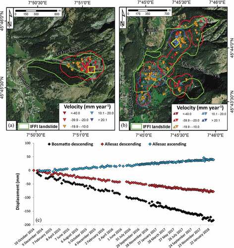
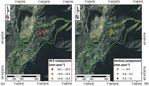
The second example (Figure 6(b)) is referred to the village of Allesaz, in the Challand Saint Anselme municipality, along with the Ayas Valley. The hamlet and its surroundings record large deformation clusters in both orbits. These moving areas coincide with the perimeter of already mapped landslides; the biggest one, that completely includes the Allesaz village, is 1.8 km long and 600 m large, being a complex phenomenon that runs from an altitude of 1800 m a.s.l. to the bottom of the valley, along with the Evançon Creek. This case study is an example of overlapping between moving areas measured in different orbits. LOS velocities reach maximum values of −20 mm year^–1 in descending orbit and 15 mm year^–1 in ascending orbit in the upper part of the landslide, at an altitude ranging between 1200 and 1300 m a.s.l. Velocities progressively decrease along the landslide, dropping below 15 mm year^–1 in both orbits. Regarding the radar reliability of the moving areas, the descending orbit cluster is classified as ‘medium reliability’ (class B in Figure 3) whereas the clusters in ascending orbit are classified as ‘low reliability’ (class C in Figure 3). This is due to a higher noise of the time series with respect to the Bosmatto case study and because of different slope orientation effects depending on the orbit. Descending data allow a better estimation of the real displacement vector, obtaining a C index equal to 0.7 (about 70% of the real motion is detectable); in ascending orbit this value falls below 60%. Considering the presence of moving areas in both orbits, it is possible to derive the vertical and horizontal (in west–east direction) components of the landslide (Tofani et al. 2013). For an explanation of the approach used we refer to Chapter 2 of the Supplementary Materials. The combination between ascending and descending data reveals that only the upper portion of the landslide registers vertical motions (with maximum velocities of −6 mm year^–1) and that the main landslide component is horizontal (SW direction). West–east velocities reach values of −28 mm year^–1 in the upper part of the landslide and −15 mm year^–1 in its central portion, on top of which the Allesaz village is built (Figure 7). These data confirm the classification of the landslide as ‘complex’, registering a main translational component with a minor rotational component. The time series of deformation (Figure 6(c), light blue and red points) referred to the upper portion of the landslide show a linear and continuous trend, like Bosmatto. The noisy periods are here limited and less evident; this is due to a climatic evidence, in fact the Bosmatto landslide is located at highest altitude (crown area at around 2700 m a.s.l.), thus characterized by more persistent snow cover during winters.

Figure 7. Horizontal (a) and vertical (b) components for the Allesaz landslide

Figure 8 shows two examples of moving areas recorded outside of known landslide boundaries, along slopes already affected by mapped phenomena. The first case study is taken from the Ayas Valley, in the homonymous municipality (Figure 8(a)). This area is characterized by three moving areas; the first one, the largest (area 1 in Figure 8(a)), is composed of 45 PS points located between Col Tantanè and Barmasc, at a height ranging from 2000 to 2600 m a.s.l. The other two areas (2 and 3 in Figure 8(a)), smaller and composed of 4 PS each, are located western than Col Tantanè, at an altitude of 2500 −2600 m a.s.l. LOS velocities of the area 1 range between −42 mm year^–1 in the northern portion and −15 mm year^–1 along its south-western border. All three moving areas can be considered as ‘highly reliable’ (class A in Figure 3) because of the values of C index (ranging between 0.86 and 0.88) and coherence of the time series. This moving area is located between two known landslides, along with a steep slope with widespread debris deposits. Considering local morphology and satellite data, we hypothesized the contour of the possible upper limit of the unstable area, as shown by the white dashed line in Figure 8(a). The time series of deformation for the area 1 shows that the movement is constant over time (red points in Figure 8(c)), with noisy periods related to the presence of snow, as shown before (Figure 6(c)). Area 2 and 3 have similar average LOS velocities (around −15 mm year^–1) and are placed near the upper limit of a mapped landslide, classified as ‘rotational slide’. Here the deformation recorded could suggest i) a retrogression of the landslide already included in the IFFI catalogue (Figure 7(a)) or ii) the motion of small unstable debris masses on top of the steep slope, not connected to the activity of the mapped phenomenon.

Figure 8. Moving areas falling outside the contours of already mapped landslides. The Sentinel-1-derived PS points are represented as triangles with downward orientation if the orbit is descending, upward if it is ascending. Red and blue contours represent moving areas in descending and ascending orbits, respectively. The white dashed lines represent possible landslide crowns traced on the basis of terrain morphology and PS data. Two examples from the Ayas (a) and Saint Rhémy En Bosses (b) municipalities are reported. (c) average time series of deformation for the sectors indicated by yellow rectangles

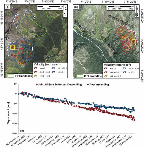
In Figure 8(b) a second example of a moving area that does not intersect landslide inventories is presented. The deformation cluster is located in the Saint Rhémy En Bosses municipality, along the Cote de Barasson at an altitude between 1900 and 2200 m a.s.l. The cluster is composed of 60 PS points with velocities ranging between −30 and −12 mm year^–1 and is classified as ‘highly reliable’ (class A in Figure 3) considering the values of C index (91% of the real displacement vector can be measured) and coherence (above 0.85 on average). The time series of deformation shows a linear trend with little winter oscillations and a slight deceleration between June and November 2015 (blue points in Figure 8(c)). This part of the Saint Rhémy municipality is affected by two large complex landslides threatening the access to one of the main connections between Italy and Switzerland, the Gran San Bernardo tunnel. Thanks to the satellite data it is possible to mark the contour of a moving area that, if completely mobilized, could hazard the state road that in the hamlet of Thoules, 300 m below the cluster of deformation, connects the Gran San Bernardo tunnel access road to the local road network.

5. Discussions

In this work, a hot-spot analysis (following the terminology introduced by Bianchini et al. 2012) has been performed in an Alpine context to retrieve areas characterized by high deformation rates, interpreting the results obtained by a geomorphological-geological point of view. This work is the first example of ground motion mapping with Sentinel-1 radar images above an entire region along the Alpine arc. The products generated, i.e. deformation maps and moving areas database, are designed for Civil Protection use, aimed at long-term reducing hydrogeological risk at regional scale. In particular, the VdA Region Geological Survey, in charge of landslide monitoring, actively uses these interferometric products as a support for early warning-detection of slope movements, coupled with meteorological and rainfall forecasting. The Geological Survey alert the Regional Civil Protection in case of anomalous motions registered by monitoring instruments; in this case, interferometric products are exploited to plan focused site surveys. If the level of risk is relevant, i.e. the population could be threatened by a geohazard detected with the proposed methodology, the Regional Civil Protection is directly involved to define proper countermeasures.

A total of 277 moving areas have been derived using a simple and reproducible approach that reduces the time needed to perform a complete analysis on thousands to millions of PS points that compose a regional-scale MTInSAR dataset (Solari et al. 2018a). Landslides and permafrost-related deformation are responsible for the detected moving areas, as already highlighted by Cignetti et al. (2016) performing ERS 1–2 and Envisat interferometric analysis over VdA.

The final output of this activity is a ‘radar interpreted’ (Farina, Casagli, and Ferretti 2007) database of deformation clusters that includes various geographical, geomorphological and geological information useful for contextualizing satellite data into the natural environment. This database, implemented in a GIS system, is delivered to regional authorities in charge of hydrogeological risk management (geological service of the Valle d’Aosta Region) and to the Regional Civil Protection. These entities actively collaborated to design the database, providing a continuous exchange of information between the University and the political sphere.

The products obtained are currently implemented in the landslide risk management chain, focusing on landslide state of activity definition and landslide mapping. The first activity can be performed using large stacks of interferometric data applying specific criteria for the definition of stability thresholds, number of PS points to be considered relevant for the designation of landslides state of activity and so on (Rosi et al. 2018). However, analyse entire interferometric datasets landslide-by-landslide and validate the evidences collected is a time demanding activity that requires time and personnel. In this work, we presented a procedure that can be finalized by a single expert in one week. Considering that the VdA IFFI database does not report the state of activity of known landslides, we can state that all the landslides (or part of them) in which a moving area is found can be considered ‘active’. Thus, a total of 92 landslides for the whole VdA territory register high deformation in the monitored time period. We estimate that the perimeter of 30% of these landslides could be modified according to the spatial distribution of the moving areas with respect to the original landslide contours and according to the local morphological features of slopes. By the way, our aim is not to update or define the activity of every landslide with PS inside (as done for the Tuscany Region by Rosi et al. 2018) but to detect only those ones with the highest deformation rates at the moment of the analysis.

Landslide mapping based on interferometric data is challenging task; in fact, due to the intrinsic limitations of the technique (presence of vegetation, topographic effects, etc…) it is difficult to obtain a complete interferometric data coverage of a landslide. Thus, landslide contours must be defined with the support of other remotely sensed data, such as multi-temporal optical images, in situ measurements and field surveys (Casagli et al. 2017). As shown by Figure 7, the deformation clusters can be used as a proxy for delimiting the spatial distribution of active motions but cannot be used to define a precise landslide contour without the help of other external data. As shown by Hölbling et al. (2012) in the case of the Ferret Valley (north-western VdA), interferometric data are useful tools for validating landslide inventories generated by means of other remote sensing techniques (in this case, object-based image analysis). In our case study, we estimate that 65 moving areas (around 50% of the total) detected outside of known landslide perimeters can be used as a proxy for new landslides definition, according to our radar interpretation of interferometric results. These areas should be anyway directly verified in situ or at least by means of a focused multi-temporal analysis of orthophotos. These data confirm the potential of our methodology as a tool for rapid mapping of slope movements at a regional scale, creating a priority list for future ground surveys and further detailed scale analyses.

Alpine regions are challenging environments for interferometric applications. It is necessary to know a priori the spatial distribution of possible ‘no data’ areas, using approaches based on the integration between morphology, land cover and satellite acquisition geometry, as the CRI here used. The results obtained are a clear reflection of the morphological limitations forced by valley orientation in the Valle d’Aosta territory. Figure 6 is an example of this. The Bosmatto landslide is in fact well detectable only in descending orbit, where 90% of the real displacement vector can be measured. This percentage drastically falls below 20% in ascending orbit. On the other hand, the Allesaz landslide is one example of slope motion that could be detected more or less in the same way in both orbits. We estimated that this type of overlapping realizes only in 20% of the mapped moving areas.

Considering topographic and land cover limitations, it is important to rank the cluster of deformations giving them a quality score (Barra et al. 2017). In this case, we defined a novel index, called ‘radar visibility index’, that intersects time series analysis (coherence index) with terrain effects on MTInSAR measurements (C index). The first index takes into account the level of noise of the time series, especially at high altitudes where the snow cover is persistent for several months (Cignetti et al. 2016). Coherence is exploited to estimate how much each measurement of the time series differs from the linear model used to calculate the velocity value of each PS. We consider that this simple statistical parameter is a good way to quickly evaluate how much is the general noise of the time series and to detect PS affected by non-linear motions. C index is introduced to evaluate the effect of slope orientation on interferometric measurements. This parameter has to be used with caution in mountainous areas, being quite sensitive to small slope orientation changes. We believe that calculating slope and aspect, necessary for deriving the C index, on a 30 m resolution DEM could limit local slope effects by smoothing the topography. Moreover, the C index is not here used for projecting LOS velocities of singles PS points along slope but as an average value referred to small areas, i.e. the deformation clusters. This is valid assuming that the PS points of each cluster are referred to the same phenomenon and to the same slope unit. Small clusters, for example, composed of three points, could have a higher variability of the C index, leading to a potential erroneous estimation of the contingency matrix.

6. Conclusions

This work presents the first example of a hot-spot analysis applied to a large stack of Sentinel-1 satellite interferometric products above a mountainous region along the Alpine arc (Valle d’Aosta, north-western Italy). Because of its peculiar climatic and morphological context, VdA is characterized by a wide spectrum of mass wasting phenomena. Our approach, based on simple GIS tools and indexes, allowed detecting 277 moving areas above the selected velocity threshold. Overall, landslides (complex, rotational, DSGSD), rock glacier evolution and debris-related deformation are responsible for the detected motions. The moving areas catalogue, produced for the period October 2014 – February 2018 but easily updatable, can be exploited for both landslide activity mapping and detection, defining more than 100 already known or new and potentially active phenomena.

This type of approach, similarly applied in different environments by some authors in the last years, allows reducing the time needed for a complete analysis of an interferometric dataset. In mountainous areas, where the field data collection is sometimes limited or impossible, the presented approach is intended to highlight priority areas to be focused for further investigations. In this way, it is possible to increase, with reduced economic and personnel costs, the ‘landslide knowledge’ (in terms of landslide state of activity estimation and mapping) of all the actors involved within the landslide risk management chain at the regional scale. The products generated are being currently implemented in the operational service for landslide management of the VdA Region, constituting a useful support for Civil Protection activities at the regional scale.

Considering the 6-days repeatability of the Sentinel-1 constellation it is possible to build up interferometric stack in shorter time than before. In this context, easily updatable hot-spot analyses with one-year repeatability are very useful tools for MTInSAR data analysts; it is possible to obtain reliable results in a fast way and to compare them with previous results.

Despite the limitations of the interferometric technique, especially in mountain regions, it is reasonable to rely on hot-spot analyses to derive multi-temporal synoptic views of ground motions over wide areas.

Acknowledgements

The authors thank the entire Tre-Altamira staff for supporting all the data processing phases, we are particularly grateful to Dr Fabrizio Novali and Dr Marco Bianchi for their support.

Disclosure statement

No potential conflict of interest was reported by the authors.

Supplementary material

Supplemental data for this article can be accessed here.

References

- Barra, A., O. Monserrat, P. Mazzanti, C. Esposito, M. Crosetto, and G. Scarascia Mugnozza. 2016. “First Insights on the Potential of Sentinel-1 for Landslides Detection.” Geomatics Natural Hazard and Risk 7: 1874–1883. doi:10.1080/19475705.2016.1171258.
- Barra, A., L. Solari, M. Béjar-Pizarro, O. Monserrat, S. Bianchini, G. Herrera, M. Crosetto, et al. 2017. “A Methodology to Detect and Update Active Deformation Areas Based on Sentinel-1 SAR Images.” Remote Sensing 9: 1002–1021. doi:10.3390/rs9101002.
- Barsch, D. 1996. “Rockglaciers: Indicators for the Present and Former Geoecology in High Mountain Environments.” In Springer Series in Physical Environment, edited by D. Barsch, 1–331. Berlin, Germany: Springer Verlag.
- Béjar-Pizarro, M., D. Notti, R. M. Mateos, P. Ezquerro, G. Centolanza, G. Herrera, G. Bru, et al. 2017. “Mapping Vulnerable Urban Areas Affected by Slow-Moving Landslides Using Sentinel-1 InSAR Data.” Remote Sensing 9: 876–893. doi:10.3390/rs9090876.
- Bianchini, S., F. Cigna, G. Righini, C. Proietti, and N. Casagli. 2012. “Landslide HotSpot Mapping by Means of Persistent Scatterer Interferometry.” Environmental Earth Sciences 67: 1155–1172. doi:10.1007/s12665-012-1559-5.
- Bianchini, S., G. Herrera, R. M. Mateos, D. Notti, I. Garcia, O. Mora, and S. Moretti. 2013. “Landslide Activity Maps Generation by Means of Persistent Scatterer Interferometry.” Remote Sensing 5 (12): 6198–6222. doi:10.3390/rs5126198.
- Bianchini, S., F. Raspini, A. Ciampalini, D. Lagomarsino, M. Bianchi, F. Bellotti, and N. Casagli. 2017. “Mapping Landslide Phenomena in Landlocked Developing Countries by Means of Satellite Remote Sensing Data: The Case of Dilijan (Armenia) Area.” Geomatics Natural Hazard and Risk 8: 225–241. doi:10.1080/19475705.2016.1189459.
- Bistacchi, A., G. Dal Piaz, M. Massironi, M. Zattin, and M. Balestrieri. 2001. “The Aosta–Ranzola Extensional Fault System and Oligocene–Present Evolution of the Austroalpine–Penninic Wedge in the Northwestern Alps.” International Journal of Earth Sciences 90: 654–667. doi:10.1007/s005310000178.
- Bovenga, F., D. O. Nitti, G. Fornaro, F. Radicioni, A. Stoppini, and R. Brigante. 2013. “Using C/X-band SAR Interferometry and GNSS Measurements for the Assisi Landslide Analysis.” International Journal of Remote Sensing 34 (11): 4083–4104. doi:10.1080/01431161.2013.772310.
- Calò, F., D. Calcaterra, A. Iodice, M. Parise, and M. Ramondini. 2012. “Assessing the Activity of a Large Landslide in Southern Italy by Ground-Monitoring and SAR Interferometric Techniques.” International Journal of Remote Sensing 33 (11): 3512–3530. doi:10.1080/01431161.2011.630331.
- Carraro, F., and M. Giardino. 2004. “Quaternary Glaciations in the Western Italian Alps-A Review.” In Quaternary Glaciations – Extent and Chronology. Part 1. Developments in Quaternary Science, edited by J. Ehlers and P. L. Gibbard, 201–208. Amsterdam, The Netherlands: Elsevier Science.
- Casagli, N., W. Frodella, S. Morelli, V. Tofani, A. Ciampalini, E. Intrieri, F. Raspini, et al. 2017. “Spaceborne, UAV and Ground-Based Remote Sensing Techniques for Landslide Mapping, Monitoring and Early Warning.” Geoenvironmental Disasters 4: 9–32. doi:10.1007/978-3-319-57774-6_18.
- Ciampalini, A., F. Raspini, S. Bianchini, W. Frodella, F. Bardi, D. Lagomarsino, F. Di Traglia, et al. 2015. “Remote Sensing as Tool for Development of Landslide Databases: The Case of the Messina Province (Italy) Geodatabase.” Geomorphology 249: 103–118. doi:10.1016/j.geomorph.2015.01.029.
- Cignetti, M., A. Manconi, M. Manunta, D. Giordan, C. De Luca, P. Allasia, and F. Ardizzone. 2016. “Taking Advantage of the Esa G-Pod Service to Study Ground Deformation Processes in High Mountain Areas: A Valle d’Aosta Case Study, Northern Italy.” Remote Sensing 8: 852–877. doi:10.3390/rs8100852.
- Crosta, G. B., P. Frattini, and F. Agliardi. 2013. “Deep Seated Gravitational Slope Deformations in the European Alps.” Tectonophysics 605: 13–33. doi:10.1016/j.tecto.2013.04.028.
- Cruden, D. M., and D. J. Varnes. 1996. “Landslide Types and Processes.” In Landslides Investigation and Mitigation - Special Report 247, edited by R. L. Schuster and A. K. Turner, 36–75. Washington, DC, United States of America: US National Research Council.
- Dai, K., Z. Li, R. Tomás, G. Liu, B. Yu, X. Wang, H. Cheng, J. Chen, and J. Stockamp. 2016. “Monitoring Activity at the Daguangbao Mega-Landslide (China) Using Sentinel-1 TOPS Time Series Interferometry.” Remote Sensing of Environment 186: 501–513. doi:10.1016/j.rse.2016.09.009.
- Dal Piaz, G. V., A. Bistacchi, and M. Massironi. 2003. “Geological Outline of the Alps.” Episodes 26: 175–180.
- De Zan, F., and A. M. Guarnieri. 2006. “TOPSAR: Terrain Observation by Progressive Scans.” IEEE Transactions on Geosciences and Remote Sensing 44: 2352–2360. doi:10.1109/tgrs.2006.873853.
- Del Soldato, M., A. Riquelme, S. Bianchini, R. Tomàs, D. Di Martire, P. De Vita, S. Moretti, and D. Calcaterra. 2018. “Multisource Data Integration to Investigate One Century of Evolution for the Agnone Landslide (Molise, Southern Italy).” Landslides 1–16. doi:10.1007/s10346-018-1015-z.
- Di Martire, D., M. Paci, P. Confuorto, S. Costabile, F. Guastaferro, A. Verta, and D. Calcaterra. 2017. “A Nation-Wide System for Landslide Mapping and Risk Management in Italy: The Second Not-Ordinary Plan of Environmental Remote Sensing.” International Journal of Applied Earth Observation and Geoinformation 63: 143–157. doi:10.1016/j.jag.2017.07.018.
- Dong, J., L. Zhang, M. Li, Y. Yu, M. Liao, J. Gong, and H. Luo. 2018. “Measuring Precursory Movements of the Recent Xinmo Landslide in Mao County, China with Sentinel-1 and ALOS-2 PALSAR-2 Datasets.” Landslides 15: 135–144. doi:10.1007/s10346-017-0914-8.
- Farina, P., N. Casagli, and A. Ferretti 2007. “Radar-Interpretation of InSAR Measurements for Landslide Investigations in Civil Protection Practices”. In Proceedings of the First North American Landslide Conference, Vail, CO, edited by V. R. Shaefer, R. L. Schuster, and A. K. Turner. Association of Engineering Geologists.
- Ferretti, A., A. Fumagalli, F. Novali, C. Prati, F. Rocca, and A. Rucci. 2011. “A New Algorithm for Processing Interferometric Data-Stacks: SqueeSAR.” IEEE Geoscience and Remote Sensing Letters 49: 3460–3470. doi:10.1109/tgrs.2011.2124465.
- Ferretti, A., C. Prati, and F. Rocca. 2001. “Permanent Scatterers in SAR Interferometry.” IEEE Geoscience and Remote Sensing Letters 39: 8–20. doi:10.1109/igarss.1999.772008.
- Fiaschi, S., M. Mantovani, S. Frigerio, A. Pasuto, and M. Floris. 2017. “Testing the Potential of Sentinel-1A TOPS Interferometry for the Detection and Monitoring of Landslides at Local Scale (Veneto Region, Italy).” Environmental Earth Sciences 76: 492. doi:10.1007/s12665-017-6827-y.
- Frey, M., J. Desmons, and F. Neubauer. 1999. “The New Metamorphic Map of the Alps.” Schweizerische Mineralogische und Petrographische Mitteilungen 79: 1–230.
- Giardino, M., and S. Ratto. 2007. “Analisi Del Dissesto Da Frana in Valle d‘Aosta.” In Rapporto sulle frane in Italia, edited by A. Trigila, 21–150. Rome, Italy: APAT Rapporti.
- Haeberli, W., B. Hallet, L. Arenson, R. Elconin, O. Humlum, A. Kääb, K. Kaufmann, et al. 2006. “Permafrost Creep and Rock Glacier Dynamics.” Permafrost and Periglacial Processes 17: 189–214. doi:10.1002/ppp.561.
- Haeberli, W., Y. Schaub, and C. Huggel. 2017. “Increasing Risks Related to Landslides from Degrading Permafrost into New Lakes in De-Glaciating Mountain Ranges.” Geomorphology 293: 405–417. doi:10.1016/j.geomorph.2016.02.009.
- Herrera, G., F. Gutiérrez, J. C. García-Davalillo, J. Guerrero, D. Notti, J. P. Galve, J. A. Fernández-Merodo, and G. Cooksley. 2013. “Multi-Sensor Advanced DInSAR Monitoring of Very Slow Landslides: The Tena Valley Case Study (Central Spanish Pyrenees).” Remote Sensing of Environment 128: 31–43. doi:10.1016/j.rse.2012.09.020.
- Hölbling, D., P. Füreder, F. Antolini, F. Cigna, N. Casagli, and S. Lang. 2012. “A Semi-Automated Object-Based Approach for Landslide Detection Validated by Persistent Scatterer Interferometry Measures and Landslide Inventories.” Remote Sensing 4: 1310–1336. doi:10.3390/rs4051310.
- Imaizumi, F., T. Nishiguchi, N. Matsuoka, D. Trappmann, and M. Stoffel. 2018. “Interpretation of Recent Alpine Landscape System Evolution Using Geomorphic Mapping and L-Band InSAR Analyses.” Geomorphology 310: 125–137. doi:10.1016/j.geomorph.2018.03.013.
- Intrieri, E., F. Raspini, A. Fumagalli, P. Lu, S. Del Conte, P. Farina, J. Allevi, A. Ferretti, and N. Casagli. 2018. “The Maoxian Landslide as Seen from Space: Detecting Precursors of Failure with Sentinel-1 Data.” Landslides 15: 123–133. doi:10.1007/s10346-017-0915-7.
- Kvam, P. H., and B. Vidakovic. 2007. Nonparametric Statistics with Applications to Science and Engineering. Hoboken, NJ: John Wiley & Sons.
- Luino, F. 2005. “Sequence of Instability Processes Triggered by Heavy Rainfall in the Northern Italy.” Geomorphology 66: 13–39. doi:10.1016/j.geomorph.2004.09.010.
- Martinotti, G., D. Giordan, M. Giardino, and S. Ratto. 2011. “Controlling Factors for Deep-Seated Gravitational Slope Deformation (DSGSD) in the Aosta Valley (NW Alps, Italy).” Geological Society London Special Publications 351: 113–131. doi:10.1144/sp351.6.
- Meisina, C., D. Notti, F. Zucca, M. Ceriani, A. Colombo, F. Poggi, A. Roccati, and A. Zaccone. 2013. “The Use of PSInSAR™ and SqueeSAR™ Techniques for Updating Landslide Inventories.” In Landslide Science and Practice, edited by C. Margottini, P. Canuti, and K. Sassa, 81–87. Heidelberg, Germany: Springer Berlin.
- Meisina, C., F. Zucca, D. Notti, A. Colombo, A. Cucchi, G. Savio, C. Giannico, and M. Bianchi. 2008. “Geological Interpretation of PSInSAR Data at Regional Scale.” Sensors 8: 7469–7492. doi:10.3390/s8117469.
- Morra Di Cella, U., S. Letey, P. Pogliotti, M. Curtaz, E. Cremonese, and M. Vagliasindi. 2011. “Nuovo catasto dei rock glaciers della Valle d’Aosta.” In Le modificazioni climatiche e i rischi naturali, edited by M. Polemio, 65–69. Bari, Italy: CNR IRPI.
- Necsoiu, M., R. N. McGinnis, and D. M. Hooper. 2014. “New Insights on the Salmon Falls Creek Canyon Landslide Complex Based on Geomorphological Analysis and Multitemporal Satellite InSAR Techniques.” Landslides 11 (6): 1141–1153. doi:10.1007/s10346-014-0523-8.
- Notti, D., J. C. Davalillo, G. Herrera, and O. Mora. 2010. “Assessment of the Performance of X-Band Satellite Radar Data for Landslide Mapping and Monitoring: Upper Tena Valley Case Study.” Natural Hazards and Earth System Sciences 10: 1865–1876. doi:10.5194/nhess-10-1865-2010.
- Notti, D., G. Herrera, S. Bianchini, C. Meisina, J. C. García-Davalillo, and F. Zucca. 2014. “A Methodology for Improving Landslide PSI Data Analysis.” International Journal of Remote Sensing 35: 2186–2214. doi:10.1080/01431161.2014.889864.
- Oliveira, S. C., J. L. Zêzere, J. Catalão, and G. Nico. 2015. “The Contribution of PSInSAR Interferometry to Landslide Hazard in Weak Rock-Dominated Areas.” Landslides 12: 703–719. doi:10.1007/s10346-014-0522-9.
- Pagliara, P., G. Basile, P. Cara, A. Corazza, A. Duro, B. Manfrè, R. Onori, C. Proietti, and V. Sansone. 2014. “Integration of Earth Observation and Ground-Based HR Data in the Civil Protection Emergency Cycle: The Case of the DORIS Project.” In Mathematics of Planet Earth. Lecture Notes in Earth System Sciences, edited by E. Pardo-Igúzquiza, C. Guardiola-Albert, J. Heredia, L. Moreno-Merino, J. J. Durán, and J. A. Vargas-Guzmán, 263–266. Heidelberg, Germany: Springer Berlin.
- Plank, S. 2014. “Rapid Damage Assessment by Means of Multi-Temporal SAR—A Comprehensive Review and Outlook to Sentinel-1.” Remote Sensing 6: 4870–4906. doi:10.3390/rs6064870.
- Raspini, F., F. Bardi, S. Bianchini, A. Ciampalini, C. Del Ventisette, P. Farina, F. Ferrigno, L. Solari, and N. Casagli. 2017. “The Contribution of Satellite SAR-derived Displacement Measurements in Landslide Risk Management Practices.” Natural Hazards 86: 327–351. doi:10.1007/s11069-016-2691-4.
- Raspini, F., S. Bianchini, A. Ciampalini, M. Del Soldato, L. Solari, F. Novali, S. Del Conte, A. Rucci, A. Ferretti, and N. Casagli. 2018. “Continuous, Semi-Automatic Monitoring of Ground Deformation Using Sentinel-1 Satellites.” Scientific Reports 8: 1–11. doi:10.1038/s41598-018-25369-w.
- Raspini, F., A. Ciampalini, S. Bianchini, F. Bardi, F. Di Traglia, G. Basile, and S. Moretti. 2016. “Updated Landslide Inventory of the Area between the Furiano and Rosmarino Creeks (Sicily, Italy).” Journal of Maps 12 (5): 1010–1019. doi:10.1080/17445647.2015.1114975.
- Ratto, S., F. Bonetto, and C. Comoglio. 2003. “The October 2000 Flooding in Valle d‘Aosta (Italy): Event Description and Land Planning Measures for the Risk Mitigation.” International Journal of River Basin Management 1: 105–116. doi:10.1080/15715124.2003.9635197.
- Righini, G., V. Pancioli, and N. Casagli. 2012. “Updating Landslide Inventory Maps Using Persistent Scatterer Interferometry (PSI).” International Journal of Remote Sensing 33 (7): 2068–2096. doi:10.1080/01431161.2011.605087.
- Rosi, A., V. Tofani, L. Tanteri, C. T. Stefanelli, A. Agostini, F. Catani, and N. Casagli. 2018. “The New Landslide Inventory of Tuscany (Italy) Updated with PS-InSAR: Geomorphological Features and Landslide Distribution.” Landslides 15: 5–19. doi:10.1007/s10346-017-0861-4.
- Salvatici, T., V. Tofani, G. Rossi, M. D‘Ambrosio, C. T. Stefanelli, E. B. Masi, A. Rosi, et al. 2018. “Application of a Physically Based Model to Forecast Shallow Landslides at a Regional Scale.” Natural Hazards and Earth System Sciences 18: 1919–1935. doi:10.5194/nhess-18-1919-2018.
- Showstack, R. 2014. “Sentinel Satellites Initiate New Era in Earth Observation.” Eos Transactions, American Geophysical Union 95: 239–240. doi:10.1002/2014EO260003.
- Singhroy, V. 2009. “Satellite Remote Sensing Applications for Landslide Detection and Monitoring.” In Landslides–Disaster Risk Reduction, edited by K. Sassa and P. Canuti, 143–158. Heidelberg, Germany: Springer Berlin.
- Solari, L., A. Barra, G. Herrera, S. Bianchini, O. Monserrat, M. Béjar-Pizarro, M. Crosetto, R. Sarro, and S. Moretti. 2018a. “Fast Detection of Ground Motions on Vulnerable Elements Using Sentinel-1 InSAR Data.” Geomatics Natural Hazard and Risk 9: 152–174. doi:10.1080/19475705.2017.1413013.
- Solari, L., F. Raspini, M. Del Soldato, S. Bianchini, A. Ciampalini, F. Ferrigno, S. Tucci, and N. Casagli. 2018b. “Satellite Radar Data for Back-Analyzing a Landslide Event: The Ponzano (Central Italy) Case Study.” Landslides 15: 773–782. doi:10.1007/s10346-018-0952-x.
- Tofani, V., F. Raspini, F. Catani, and N. Casagli. 2013. “Persistent Scatterer Interferometry (PSI) Technique for Landslide Characterization and Monitoring.” Remote Sensing 5: 1045–1065. doi:10.1007/978-3-319-05050-8_55.
- Tomás, R., R. Romero, J. Mulas, J. J. Marturià, J. J. Mallorquí, J. M. Lopez-Sanchez, G. Herrera, et al. 2014. “Radar Interferometry Techniques for the Study of Ground Subsidence Phenomena: A Review of Practical Issues through Cases in Spain.” Environmental Earth Sciences 71: 163–181. doi:10.1007/s12665-013-2422-z.
- Torres, R., P. Snoeij, D. Geudtner, D. Bibby, M. Davidson, E. Attema, P. Potin, et al. 2012. “GMES Sentinel-1 Mission.” Remote Sensing of Environment 120: 9–24. doi:10.1016/j.rse.2011.05.028.
- Trigila, A., C. Iadanza, and D. Spizzichino. 2010. “Quality Assessment of the Italian Landslide Inventory Using GIS Processing.” Landslides 7: 455–470. doi:10.1007/s10346-010-0213-0.