Using machine learning algorithm and landsat time series to identify establishment year of para rubber plantations: a case study in Thalang district, Phuket Island, Thailand

ABSTRACT

In this study, we investigated the potential of using decision tree Machine Learning (ML) algorithm and profiles of vegetation and moisture indices extracted from Land Remote-Sensing Satellite (System, Landsat) time series to identify the ages of rubber plantations in Thalang district, Phuket province, southern Thailand. The secondary Land Use and Land Cover (LULC) data and historical imagery from Google Earth^TM were used to distinguish plantation boundary and the establishment year of rubber plantation (T₀). The inter-annual profiles of spectral indices for each rubber plantation were obtained from 129 Landsat images (summer period from October 1991 to April 2018). The predictors were generated from summary distribution values of spectral indices during summer, including their difference and ratio at two years before to six years T₀ for Recursive Partitioning (RP) supervised classification algorithm. Modelling dataset from ‘known T₀’ plantations was divided into the training and testing datasets with a 60:40 ratio. The training model was 30 times repeated training while cross-validation assessment was tested to optimize an appropriated hyperparameter based on F₁ score. Then, the best performance training model was applied to both modelling and predicting (‘unknown T₀’ plantations) datasets. The predicted T₀ for each plantation was selected based on results aggregation of 100 times repeated prediction. The results show that the RP model with a complexity parameter as 0.01 and the predictors generated only from Normalized Difference Vegetation Index (NDVI) profile acceptable achieves an accuracy of 84.4% and 84.7% for lowland and highland modelling datasets, respectively. The root means squared error (RMSE) of predicted establishment year were 0.83 years at plantation scale.

1. Introduction

Para rubber tree (Hevea brasiliensis) is befittingly growing in the twelve-month rainfall tropical region within the equatorial zone between 10° N and 10° S. With modern agricultural technologies and advance agriculture knowledge, rubber trees today can be grown and cultivated in numerous locations that have tropical monsoon climate with two distinct seasons – rainless and continuous several months rainfall periods. Thus, rubber plantations have expanded rapidly to other non-traditional rubber growing region, including southern China, eastern Myanmar, northern Laos, northern Laos, northeast Thailand and Cambodia (Chen et al. 2018b). Para rubber is one of the significant economic crops in many countries in the South East Asian Nation (ASEAN) region both in terms of income and employment (Koedsin and Yasen 2016). The need for accurate information for predicting national rubber productivity is compulsory for national economic and government policy. Age of rubber tree is one of the other factors that could be used to estimate yield performance.

So far, several remotely sensed approaches had been used to obtain rubber plantation age from remote sensing data. Many previous studies achieved mapping rubber tree growth using statistical models, and image classification (Dibs, Idrees, and Alsalhin 2017; Trisasongko 2017; Razak et al. 2018) approaches, which assumed a good relationship between spectral/structural features of the plantation canopy and rubber stand age (Chen et al. 2018a). By using a single Land Remote-Sensing Satellite (System, Landsat) imagery, Chen et al. (2012a) and Suratman et al. (2004) mapped rubber plantation age from Landsat Thematic Mapper (TM) using a regression approach with Root Mean Square Error (RMSE) of 5.96 and 4.38years respectively. Applying the combination of Object-Based Image Analysis (OBIA), Vegetation Canopy Density (VCD), plant phenology, and intensive ground observation to two pansharpened and multispectral image sets from Thailand Earth Observation System (THEOS), Putklang, Mongkolsawat, and Suwanwerakamtorn (2019) achieved a classification of four stages (< 1, 1 to 4, 4 to 7 and > 7 years) of rubber plantation with an overall accuracy of 79.0% and Cohen’s Kappa Coefficient (K) of 0.77. Moreover, modern Machine Learning (ML) algorithm was implemented in pixel-based image classification approaches. Chen et al. (2012b) apply artificial neural networks to estimate rubber stand age using 30 m resolution Landsat TM. They can achieve high accuracy of rubber tree stand age prediction compare to classical regression approach. Koedsin and Huete (2015) used even finer spatial resolution Pléiades imagery (0.5 m) incorporate with a supervised maximum likelihood classification. The classifier was able to classify plantation age classes for < 7 (pre-production), 7 to 15 (young plantation) and > 15 (mature plantation) years with an accuracy of 96.61%. However, classification of a single or few satellite imagery using vegetation indices and multispectral bands cannot accomplish identifying the age of rubber trees with precise annual resolution.

Many previous studies focus on developing biophysical and yield models for precision farming from multiple historical satellite images (e.g. Thenkabail 2003). Li and Fox (2012) explored the potential of combining 29 Moderate Resolution Imaging Spectroradiometer (MODIS) vegetation index time series with national statistical data to map the distribution of rubber tree growth across mainland Southeast Asia landscape. Vegetation phenological analysis based on Normalized Difference Vegetation Index (NDVI) was possible to accomplish with the dense time series from MODIS, but its coarse spatial resolution (250 m) was unsuitable to the small-scale rubber plantation, especially in Thailand where smallholders produce around 85 to 90% of rubber (Chen et al. 2018b; Chantuma et al. 2011). With the higher spatial resolution, multi-temporal 30 m Landsat imagery had proved a success in several studies of rubber mapping (e.g. Dong et al. 2013; Grogan et al. 2015). Temporal cross-sensor Landsat imagery over several years makes it possible to pixel-scale map the establishment year (stand age) of rubber plantations at annual resolution using Land Use and Land Cover (LULC) change detection on dense Landsat time-series data. (Kou et al. 2015) firstly presented the best-available-pixel (BAP) composites method, they successfully mapped a five-year rubber plantation stand age in small and entire Xishuangbanna province – the second largest rubber planting area located in southern of China – (Kou et al. 2018). Beckschäfer (2017) further developed the BAP method with aggregated 270 Landsat TM and Enhanced Thematic Mapper Plus (ETM+) surface reflectance images. The time of plantation establishment was identified by selecting images from the foliation phase for rubber trees and selecting the last occurrence of a no-vegetation pixel (bare soil) based on a global Normalized Difference Moisture Index (NDMI) threshold of 0. This land cover changed detection approach achieves mapping rubber plantations at annual scale in Xishuangbanna province with RMSE of 2.5 years. Chen et al. (2018a) also successfully used exposed soil during plantation establishment and linear increases of canopy closure during the non-production period to monitor the establishment of rubber plantations. Not only used a single global cut off value which the minimum NDMI during defoliation period less than zero, but they also used the slope coefficient of linear increasing of NDVI values during growing phase (8 years from seeding to maturity) as the conditions algorithm. The slope criterion was initially set as 0.03 after statistically calculated from the training samples. With the frequent presence of clouds and difficulty of a ground survey to getting information in young rubber plantations, however, they re-adjusted the algorithm again with slightly higher thresholds of 0.1 for minimum NDMI and 0.02 for the increasing slope of greenness to address the less optimal conditions. Despite finding and statistically adjusting optimal condition values, they mapped the establishment year of rubber plantations on Hainan Island, China, with the coefficient of determination (R²) = 0.85 and RMSE = 2.34 years at pixel scale, and R² = 0.99 and RMSE = 0.54 years at plantation scale. Integrated pixel- and object-based tree growth model proposed by Chen et al. (2018b) can produce a rubber stand age map cover tri-border region along the junction of China, Myanmar and Laos with 87.0% accuracy and an average error of 1.53 years in age estimation. They mapped the stand age of rubber plantations by selecting candidates as the starting year of rubber cultivation from NDVI time series where its values were smaller than 0.4. They then fitted the pre-developed tree growth model based on the logarithmic function to assesses the potential starting year and finally with two criteria regarding optimal value and variation of model parameters. Moreover, Ye, Rogan, and Sangermano (2018) introduced a new two-step classification procedure. They, first, detected the ‘shapelet’ window in a Landsat-NDVI time series using developed shapelet detection algorithm and then determined whether the means of NDVI for shapelet window and non-shapelets parts in time series were significantly different using paired-sample t-test. The proposed method can produce rubber plantation map in Seima Protection Forest in Cambodia with an overall 89% accuracy. Similarly, Xiao et al. (2020) developed a tri-temporal windows algorithm based on the characteristic of a rabid phenological transition period to map deciduous rubber plantations in northern Laos region. They first used the combination of spectral indices thresholds were defined to distinguish rubber plantations from natural forest and then applied the windows algorithm on a sequent of the 10 Landsat Operational Land Imager (OLI) images during 2013 to 2016 to find the time of significant defoliation phase. The difference values of Normalized Burn Ratio (NBR) from pre-defoliation stage to defoliation stage, i.e., a senescence period and from defoliation stage to foliation stage, i.e., a re-greening period were determined. If the change in NBR from both senescence and re-greening periods large than 0.35, the pixels were classified as rubber plantations and vice versa.

Many relevant previous studies demonstrated the success of using threshold criteria and phenology-based models together with satellite images time series to map rubber stand age in various rubber cultivation regions. However, in the tropical area where the predominant defoliation phase of rubber trees may not present, as well as in different local rubber agriculture practices areas, could cause a high variability of phenological phase. The use of single and integrated global thresholds or other pre-defined conditions based on the phenology of rubber plantations may require specific adjustments and challenging to find the optimal cut-off figures in a complicated pattern of phenological profile. Here, we investigated the using of a simple tree-based ML algorithm, called Recursive Partitioning (RP), incorporated with a vegetation transition and a soil exposure signatures during two years before and six years after the establishment of rubber plantation to map the age of rubber plantation in a small tropical study area of Thalang district, Phuket island, Thailand.

2. Materials

2.1. Study area

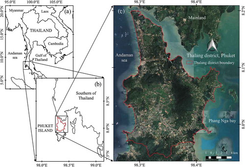
Thalang District, the northern part of Phuket Island, is the study area for this study Figure 1. Phuket Island is the largest island situated off the southwest coast of Thailand, known as the Andaman Sea region. The climate in the study area is tropical monsoon with distinctively dry and rainy seasons. The northeast monsoon begins in November and usually lasts until March which brings cold and dry air from the Asian continent and causes the dry-season aridity in the Andaman Sea region. The rainy season (April to October) with continuous high precipitation is caused by the strong wind of the southwest monsoon which draws warm moisture from the India Ocean. After the end of the tin mining industry in the early 1990s, natural latex from the Para rubber tree is one of the primary sources of income for the local villagers. The majority of the lowland area on the Phuket island had been turned to rubber plantation as a replacement for the tin mining business (Chaiyarat 2007). Phuket island is known as the famous tourist destination nowadays, and the tourism sector contributes most of its income. Despite many developments in infrastructure and commercial property, to support the rapid growth of the tourism industry, there are still many productive plantations, especially in the Thalang district area. More than 90% of rubber planning areas in the study area, also similar throughout Thailand, were established and are managed by smallholder farmers.

Figure 1. (a) Map of Thailand, (b) Phuket Island in southern Thailand and (c) the area of Thalang district.

2.2. Rubber planting practice

According to the Good Agriculture Practices (GAP) for rubber guidelines (Prommee et al. 2018), the rubber tree planting in the study area, same as other places around Thailand, occurs regularly around the end of the local dry period and continues during the early local rainy period. Land clearance is a prerequisite of the rubber seedling. The process of land preparation typically starts around mid of the dry period when the ground is solid enough for heavy machinery. The plantations in lowland usually have been turned into completely bare land, but land preparing process for plantations located in foothill and steep areas is different. The ground usually has been cleared and levelled as a terraced track along the contour of the hillside. The tracks are around 2 to 4 m apart, which depend on the steepness of the land, and some vegetation is left between the tracks. Thus, the highland plantation is terraced land covered by a mixture of sparse vegetation and bare soil.

In Thailand, the rubber-based agricultural system is characterized by three main categories (Simien and Penot 2011): (i) the ‘jungle rubber’ system, which is gradually being abandoned by the farmers, (ii) the monoculture system, which is now the most widely-used system in Thailand and (iii) the intercropped system, based on an association with different crops (fruits, vegetables, cereals) and economic trees (teak, bamboo). The crop-rubber associated plots were found throughout the study area, especially in the lowland. The dominant intercropped plant found in the study area is pineapple fruit. It was introduced, along with other herbaceous plants, to the local smallholder farmers and they were encouraged to grow the pineapples between the rubber tree rows at the beginning or during the first four years of plantation establishment. The ‘short-term’ intercropped approach was adopted to reduce the environmental and economic risk that could subsidies the household incomes during the unproductive stage of rubber culture in the first four to five years.

2.3. Data

2.3.1. Land use and land cover

The secondary LULC data of the year 2016 used in this study were acquired from the Land Development Department (LDD), Ministry of Agriculture and Cooperatives of Thailand. The obtained LULC data are in vector format. There are five main classes of land cover classified by LDD and the rubber agricultural land use in the original LULC data were marked with Level-3 LULC code as ‘A302ʹ. There are approximately 89.29 km² of rubber plantation area in the 284.53 km² area of the Thalang district. The plantations are spread over the flat lowlands land and many of the steep foothill areas. According to the local GAP for rubber cultivation, we classified rubber plantations into two main groups, ‘lowland’ and ‘highland’, where lowland plantations are situated in the areas that are lower than 50 m above sea level and have a slope less than 15%, and the highland plantations are otherwise.

2.3.2. Landsat imagery

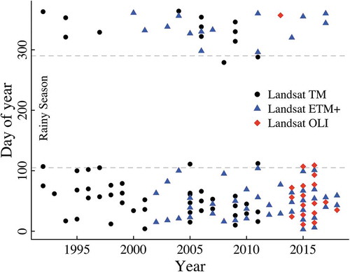
The main goal of this study is to determine the year of rubber plantation establishment from the inter-annual spectral indices profile. The time of land clearance and the rubber tree planting in the study area usually happen during the summer period according to local GAP of rubber cultivation, described in Section 2.2. Thus, the multi-temporal Level-2 Landsat Surface Reflectance (SR) TM, ETM+, and OLI products at Worldwide Reference System 2 (WRS-2) path 130, row 54 that available during the dry season (day of year 280 to 120 of the following year) were acquired through the Earth resources observation and science (EROS) center science processing architecture (ESPA) on demand interface (https://espa.cr.usgs.gov). The first available image dates were from 16 March 1992, and the last image dates for 4 February 2018. However, only 129 images with cloud cover below 20% over the study area were selected for the study. There are 55 Landsat TM images, 56 Landsat ETM+ images, and 18 Landsat OLI images, as illustrated in Figure 2. The acquired surface reflectance images were used to calculate NDVI, Enhanced Vegetation Index (EVI), Soil Adjusted Vegetation Index (SAVI), and Normalized Difference Moisture Index (NDMI).

Figure 2. Acquisition dates of the 129 Landsat TM, ETM+ and OLI images.

2.3.3. Registration of rubber farmer

Registrations of rubber farmers in Thalang district were obtained from the Rubber Authority of Thailand (RAOT), Phuket Province (www.rubber.co.th/phuket/). RAOT is the government agency under the Ministry of Agriculture and Cooperatives of Thailand, which responsible for administration and management of the entire system of rubber production in Thailand on an integrated basis. The documented registrations for rubber plantations in the study area were collected from 2013 to 2018. There were 154 records which consisted of landowner information, Universal Transverse Mercator (UTM) Zone 47 coordinates of plantation shape, coordinates at the middle of the plots, location and size of plots, as well as the year of registration and approval of cultivation from RAOT. The geographical information was used to update LULC data, along with historical imagery from Google Earth^TM, whereas the information of approval year were used for prediction validation. However, registers data with approval year in 2018 (collected around March 2018) were omitted because many farmers had cleared the land but planned to re-plant the rubber trees in the following planting season. Thus only 124 register records were used in mapping accuracy assessment.

3. Methodology

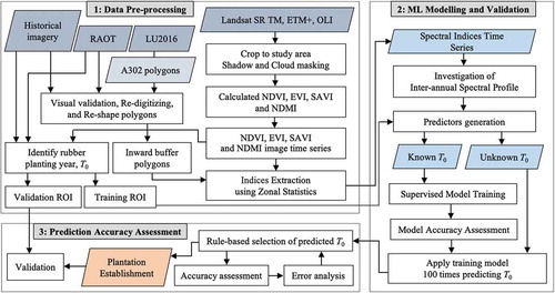
In this study, there were three main steps: 1) data pre-processing, 2) machine learning modelling, and validation, 3) prediction accuracy assessment, as illustrated in the following flowchart Figure 3. The processes in the second and third steps were performed for plantations in lowland and highland separately.

Figure 3. Flowchart of methodology.

3.1. Data preprocessing

3.1.1. LULC data

The secondary LULC vector data were selected only the polygons that were identified as para rubber land use (labelled as ‘A320ʹ) in Level-3 LULC classification, including one that blends with other unseasonal crops such as pineapple and banana. The polygons were then verified with Historical High Resolution (HHR) images available via Google Earth^TM and the coordinates of plantation data from RAOT to ensure the LULC database is up to date (up to December 2018). In this early step, visual interpretation of HHR images is the essential technique in the process of updating the obtained vector data. A vegetation clearance footprint, including the unique patterns of rubber tree planning (mixed with pineapple in the early years of growing phase), rubber tree canopy, and rubber tree spacing were used to distinguish the plantation boundary. Re-digitizing and re-shaping plantation polygons were carried out when necessary on both Google Earth^TM and Quantum GIS (QGIS) platform (QGIS Development Team 2018) for the most accurate representation of rubber plantation areas. The historical satellite images also were used to identify the time (dry season) of land preparation for rubber planting, which will be used as labelled data in the ML supervised model training process.

3.1.2. Spectral indices and spectral time series extraction

All 129 Landsat Level-2 SR images were cropped to the study area. To minimize the influence of negative atmospheric noise and image anomalies, the pixels that labelled as clouds, cloud shadows, and water which corresponding to the product pixel quality attribute was masked from the corresponding images. Also, the gap pixels in the obtained Landsat 7 ETM+ with failed Scan Line Corrector (SLC) data were replaced with ‘NA’ before the extraction of spectral index time series. NDVI, NDMI, and NBR were offend used in previous studies for mapping rubber plantation and classifying rubber stand age. According to the local GAP, there is no activity of using fire to clear land in our study area. Thus, we considered not to use NBR but using EVI and SAVI as additional vegetation indices (VIs). EVI might be a good candidate in this case because we are focusing on dense vegetation cover of fully grown rubber plantations, as well as, the spread vegetation area of young rubber plantations in which SAVI cloud performs better than NDVI to quantify vegetation greenness. In this study, NDVI, EVI, SAVI, and NDWI were derived from the cropped and cloud-free Landsat SR images. The definitions of the vegetation indices and moisture index, including their calculation formulas for Landsat imagery are detailed in Landsat Spectral Indices Product Guide (Masek et al. 2006; Vermote et al. 2016).

Afterwards, for each spectral index, all derived images were extracted using ‘Zonal Statistics’ in QGIS software. Before spectral index extraction, all updated rubber plantation polygons, as described in Section 3.1.1, were shrunken using inward buffering by 15 m to exclude the spectral values from pixels that are situated at the plantation edge. Elimination of edge effects is essential to minimize the influence of spectral noise signal from adjacent plantations and adjacent land uses. Then, the average of spectral values, which represented the overall spectral value at plantation scale, from all pixels within each shrunken polygon were determined for each Landsat image. The output from the process of the spectral value extraction was the tables contain the plantation’s ID attribute and 129 attributes of mean spectral value which calculated from all Landsat images ordering by acquisition date.

3.2. Machine learning algorithms and model validation

3.2.1. Predictors

We considered using the characteristic of inter-annual spectral index profile in identifying plantation establishment year. There is a high variability of spectral index values during the dry season due to local climate variability, rubber tree structure, elevation, ground moisture, soil properties (Dong et al. 2013), local rubber GAP, as well as availability and signal quality of Landsat images. Using mean, minimum, or maximum of spectral index values within the same dry season to represent yearly spectral index profile might not be appropriated. The minimum or maximum values among within-dry-season spectral index values can be outliers and the mean value, as the measures of central tendency, is unusable when the extreme values are presented. Therefore, we used all information of dispersion (or variability): (i) inter-quartile range (IRQ), (ii) first quartile (Q₁), (iii) third quartile (Q₃), (iv) median, (v) minimum (Q₁ – 1.5 × IRQ), and (vi) maximum (Q₃ + 1.5 × IRQ) to represent yearly spectral index profile. In order to obtain the inter-annual spectral index profile, 129 spectral values in spectral index time series were aggregated into 27 groups corresponding to their acquisition date which falls within 27 dry seasons (between Julian day 280 to 120 of the following year) during the study period. Six distribution summary values were computed from same-season spectral values for all 27 dry seasons.

Consequently, each plantation has 27 data records, and each record initially contains six distribution summary values as the predictors. To take advantage of time series data and the characteristic of spectral signature betweentwo years before (T₋₂ and T₋₁) to six years 6 years after (T₁ to T₆) the plantation establishment (T₀), the predictors were generated from difference and ratio of significant distribution summary values among different years to capture the structure of yearly spectral index trend of rubber plantation establishment. The additional variables were comprised of (i) minimum value at a particular year subtracted with the maximum value at other two years before, and six years after a particular year, (ii) Q₁ at a particular year subtracted with Q₃ at other eight years 8 years, and (iii) Q₃ at other eight years divided by median at a particular year. Moreover, we also considered the characteristic of rapid transition of a yearly trend. The breakdown of the inter-annual trend of vegetation and land cover moisture was determined from the decreasing slope of linear line connected median of spectral index values within T₋₂ and T₋₁ year to T₀ year. Similarly, the increasing linear trend during 6 years plantation greening up phase was also calculated in the same manner. Finally, the structure of data consists of plot ID, year (1 to 27), the six distribution summary values, and 32 additional predictors used for model training and prediction.

3.2.2. Supervised model training

The predictor data were separated into modelling (or ‘known T_0ʹ) and predicting (or ‘unknown T_0ʹ) datasets where the ‘known T_0ʹ dataset contains all data from plantations that know the year of land clearance preparing for rubber planting. This information was obtained from the process of identity rubber planting year using Google Earth^TM historical images in the early state of LULC data preparing. For each plantation in the ‘known T_0ʹ dataset, the binary status of land clearance activity, appear (1:Yes) and not appear (0:No) at a particular year, was assigned to each 27 years vegetation and moisture indices profile as an outcome variable.

To explore an advantage of tree-based model ML algorithm, we decided to use RP as a simple algorithm to built the decision tree. This decision tree classification models are a popular method for various machine learning tasks. RP is a statistical tree-based method for multivariable analysis (Izenman 2013). It creates a decision tree to split members of the population recursively into sub-populations based on the independent variable (or predictor) that results in the most significant possible reduction in the heterogeneity of the predicted (dependent or outcome) variable, in case of categorical classification (Breiman et al. 1984). The splitting ends when a predetermined termination criterion is reached. The Complexity Parameter (CP) is the only model hyperparameter used to control the size of the decision tree and to select the optimal tree size in this RP algorithm. As our outcome variable is a categorical response, we implemented a classification tree method using R ‘rpart’ package (Therneau, Atkinson, and Ripley 2018). The algorithm of growing a classification tree is recursive binary splitting the training observations in the aim of predicting that each observation belongs to the most commonly occurring class. The RP algorithm was adopted in this study because of its simplicity of model tuning with only one hyperparameter and the extremely rapid perdition because no complex mathematics is further required after the model has been developed (Maxwell, Warner, and Fang 2018). Furthermore, the ability to handle missing values in training and predicting datasets is another main reason. The approach of generating predictors to capture the inter-annual spectral profile of rubber planting occurrence involves calculating difference and ratio of distribution summary values at a particular year to other values at two years before (T₋₂ and T₋₁) to six years (T₁ to T₆) after. The difference and ratio values on a particular record were related to other records. Moreover, their values at first two and the last six of the 27 records of each plantation cannot be computed and marked as missing values. The generated predictors were missing, not at random. In this circumstance, trying to fill missing data based on the measure of central tendency of non-missing values in a variable, as implemented in the most popular random forest (Tang and Ishwaran 2017), is meaningless and could lead to a low quality of training dataset.

To investigate the potential of RP classifier with different hyperparameter and sets of predictors, the model selection process was performed by randomly dividing the dataset into training, and testing sub-dataset by 60% and 40% of the number of plantations that know T₀, respectively. Test dataset was used to select the most appropriate model by evaluating the performance of the models via F₁ score, which often used in the evaluation of binary classifiers (Powers 2011). Also, the testing dataset was used to detect overfitting and account for the generalization of the model. In general, the model that has a relatively high evaluation matrix (or low error matrix) in both datasets and have similar or not very different values is the promising candidate. The balanced F₁ score was unitized in this study because the predicted classes were skewed. We classified the binary outcome as ‘1:YES’ (3.7%) where land clearance preparing for rubber planting was found, and ‘0:NO’ (96.3%) otherwise. This score takes both False Positive (FP) and False Negative (FN) into account when measuring the quantity of True Positive (TP) in the confusion matrix. The formula of F₁ score defines as

(1) $F_1=2\times \frac{R\times P}{R+P}$(1)

where $R=\frac{\left(\mathrm{T}\mathrm{P}\right)}{\left(\mathrm{T}\mathrm{P}\right)+\left(\mathrm{F}\mathrm{N}\right)}$, $P=\frac{\left(\mathrm{T}\mathrm{P}\right)}{\left(\mathrm{T}\mathrm{P}\right)+\left(\mathrm{F}\mathrm{P}\right)}$

The training of the model was repeated for 30 times to find an appropriate hyperparameter and set of predictors that give the best performance. Then the classifier (predicting model) with the chosen CP and set of predictors, which learned from ‘known T_0ʹ dataset was applied on ‘unknown T_0ʹ dataset.

3.3. Error analysis and ensemble methods

The processes as described in Section 3.2 were separately conducted on both lowland and highland datasets. For each dataset, the classification was repeated for 100 times. The results from each time of prediction were aggregated, and the final result was nominated based on the condition defined to select the aggregated results. The conditions were set after error analysis (Ding and Sheng 2010; Bannach-Brown et al. 2019) on particular cases of misclassification and aimed to produce the highest accuracy result. The purpose of error analysis is to manually examine the examples of misclassified result and find the systematic trend in which type of examples that the algorithm is making an error on. The concept of ensemble method is the combination of several supervised learning models that are individually trained, and the results merged in a various way to achieve the final prediction (Polikar 2006; Rokach 2010; Zhou 2012). Finally, the combined result from lowland and highland datasets was evaluated to assess the efficiency and usefulness of the classification output.

3.4. Prediction accuracy assessment

For this study, the region of interest (ROI) samples for evaluating the accuracy of identifying the age of rubber plantation were a combination of (i) rubber farmer registration data obtained from RAOT and the establishment year of rubber plantation visually interpreted using (ii) HHR imagery from Google Earth^TM and (iii) time-series NDVI and NDMI images derived from Landsat imagery. Due to different availability of reference data, ROI samples from farmer registration records were used to find rubber plantation age after 2013, whereas ROI samples from Google Earth^TM were used to find rubber plantation age after 2002. The visual interpretation of time-series NDVI and NDMI imagery provided ROI samples of rubber plantation established from 1992, which is the first year of Landsat imagery acquisition. However, stratified random sampling grouped by years of plantation establishment was used to select haft of ROI samples from all three sources of reference data for tree-based algorithm training, and the rest were used for validation. We calculated the mean and standard deviation of the predicted establishment year group by year (Chen et al. 2018a). Then, the group means and standard deviation of predicted establishment year of rubber plantations were plotted against observed year.

4. Result and discussion

4.1. Spectral index time series analysis

Figure 4 (a – e) demonstrates the inter-annual NDVI profile of the example lowland intercropping plantations and highland monoculture plantations, respectively. The spectral index time series were starting from October 1991 to April 2018. The label ‘n:’ indicates the number of acquired Landsat images, and the boxplots demonstrate the dispersion of average spectral index values extracted from multiple Landsat images during the dry season of each year. Three HHR images display the dynamic of the plantation at before, at the time of land clearance, and a few years after rubber tree planting. The observed NDVI values, in this example, should be around 0.8 to 0.9 at the beginning of summer because there is a high possibility that the land cover is the dense canopy rubber trees in case of re-cultivation or the pristine dense-evergreen and tropical rain forests in case of new planting. During the land clearing/vegetation clearances process, vegetation index should be around below 0.2 to 0.3 for a couple of months before gaining up to around 0.5 after planting rubber trees mixed with pineapple. However, the interval of each three sub-periods in the rapid transition of yearly trend period can be varied, which cause a skewed dispersion of NDVI values in the rainless period.

Figure 4. Inter-annual NDVI profile of example (a) intercropping lowland plantation and (e) highland plantation. The high resolution images from GoogleEarth^TM show three phases of lowland plantation when (b) before land clearance year (8 January 2004), (c) at year of land clearance (23 February 2009), and (d) after the year of land clearance (28 January 2014). Also the three-phase aerial images of highland plantation at (f) 14 September 2002, (g) 8 January 2004, and (h) 23 February 2009.

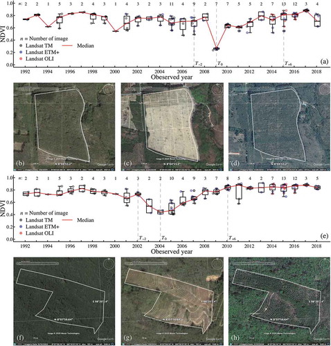
The breakpoint of inter-annual vegetation trend in the lowland plantation was noticeable when the annual spectral value drops approximately below 0.4, which associated with the historical Google Earth^TM images. The spectral values breakdown in the highland plantation was not conspicuous, where the spectral values at land clearance time remained higher than 0.4. However, there is a visible and persistent pattern of inter-annual NDVI trend during six years of rubber tree growing from the time of planting to the closed-canopy rubber trees, as shown in Figure 5. Typically, the yearly NDVI profile of rubber planting and growing phase in highland is higher than in lowland due to the difference of the local rubber GAP described in Section 2.2. Figure 5 also demonstrates the comparison of the yearly vegetation trend during two years before (T₋₂) and six years after (T₊₆) the rubber tree planting year (T₀) between highland and lowland plantations. The profile of other EVI, SAVI, and NDMI behave similarly to NDVI, but only the magnitudes of their values were lower than. The downward values of NDMI at T₀ could reach a negative scale in some plantations in case that if the Landsat images capture the completed land clearance of the entire plantation area. If vegetation cover remains in some parts of plantation extend during the land clearance processing when the Landsat image was taken, the average NDMI value may not reach below zero.

Figure 5. Comparison of inter-annual NDVI profiles for 30 sample lowland and highland plantations during two years before rubber tree planting (T₋₂ to T₋₁), the year of rubber planting (T₀), and the growing period (T₊₁ to T₊₆).

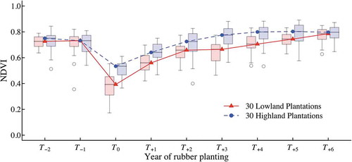
We also found that there was a steady increasing linear trend of spectral index during the first six years of non-productive period in most of the 13 sample monoculture lowland plantations. In contrast, significant dissimilarity of this trend was noticeable in all 17 intercropped lowland plantations, as detailed in Table 1. The primary cause of this high variation was the practice of intercropped pineapple planting. This tropical plant tropically takes up to two years to grow and produce edible fruit. The intercropped system rubber framers can plant pineapple at the same time of rubber seeding year (T₀) and then harvesting fruit next two years (T₊₂). They could repeat planting for the other harvesting years (T₊₄) if the canopy of the rubber tree is not fully cover and allows the sunlight gets through on the ground. Thus, there was a sign of dropping values at T₊₂ and T₊₄ in spectral index profiles. Planning this non-seasonal crop can begin at any time. However, many farmers often plant pineapple right between the very end of the dry season to the beginning of the rainy season, as well as to apply special fertilizers to speed up fruit yield period (1.2 to 1.5 years), for earning higher prices of their off-season product. This key factor directly contributes to variation of increasing slope and within-dry-season distribution of spectral index values during six years of rubber tree growing.

Table 1. Statistical information for the slope coefficient of spectral indices values during the first six years of non-productive phase in 30 sample lowland rubber plantations.

	Rubber-based agricultural system
Spectral Index	Monoculture		Intercropped
	µ	σ	µ	σ
NDVI	0.075	0.008	0.066	0.015
EVI	0.070	0.011	0.063	0.018
SAVI	0.072	0.009	0.070	0.020
NDMI	0.076	0.009	0.074	0.019

µ indicate mean values, and σ stands for standard deviation

4.2. Hyperparameter and predictors

Figure 6 (a,b) illustrates the results from the sensibility test of various sets of predictors that varies by different CP and the importance of predictors, which used in model training of 30 times performance cross-validation. In lowland dataset, there is insignificant different of model performance across different sets of predictors derived from individual and combined spectral indices and the various CPs (mean F₁ = 0.658), excepting a set of predictors derived from only NDMI (mean F₁ = 0.534), as shown in Figure 6a. This similar F₁ score characteristic also found in the highland dataset, as shown in Figure 6b. As NDMI is sensitive to moisture (Grogan et al. 2015), the healthy green vegetation could have high, positive value and non-vegetation land surface, such as bare soils could have a negative value (Watmough, Atkinson, and Hutton 2011). Although, the negative spectral value depicts plantations that were soil exposed during the observed dates.

Figure 6. The 30 times performance sensibility test on various sets of predictors varies by five complexity parameters for (a) lowland and (b) highland datasets. And the frequency of utilized predictors in sensibility tests in case of using (c) only NDVI and (d) all indices for lowland dataset, and (e) only NDVI and (f) all indices for highland dataset.

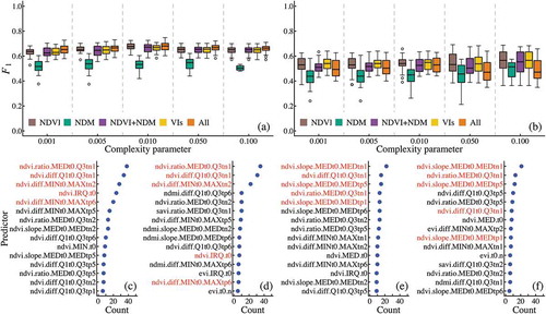
According to the local GAP in the study, the land clearance process could take time, which depends on the extent of the plantation. Some small to medium plantations operated by smallholder might take two to three weeks to finish ground cover clearance, especially in case of a re-planting plantation. The farmers carefully and slowly harvesting rubber timber for the last income offered from the non-productive plantation, which will turn, part by part, the green land cover gradually to bare soil. The plantation may not have thoroughly non-vegetation cover when the imagery was acquired. Therefore, this effect of heterogeneous land cover inside plantation extend could vary the average value (positive or negative) as we used to represent the spectral index value at the particular plantation and at the time of image acquisition. Consequently, the predictor calculated from different or ratio of the summary distribution values for both positive and negative NDMI could be immensely varied. These results from the sensibility test imply that the predictors derived from the NDMI profile, in this case, were unsuitable for both lowland and highland datasets.

Figure 6 (c – f) shows the list of predictors order by their frequently used in RP model training on the set of predictors calculated from only NDVI and all indices for lowland and highland datasets. In general, there were three distinctive predictors derived from NDVI profile; (i) ratio of the median at T₀ by Q₃ at T₋₁, (ii) difference of Q₁ at T₀ and Q₃ at T₋₁, and (iii) difference of minimum at T₀ and maximum at T₋₂ that had been repeatedly used in forming decision tree in lowland data modelling. These results indicate that the pattern of greenness breakdown in the rapid transition phase of the yearly trend (T₋₂ to T₀) gives essential information to the learning RP algorithm. Moreover, the top three often used predictors in both sets of ‘only NDVI’ and ‘All Indices’ predictors were ranked as the same. It suggests that only predictors derived from the NDVI profile were enough for the best performance of modelling the lowland dataset.

In the highland dataset, the declined rate and amount of greenness breakdown was the most important predictors. However, the increasing rate and amount of vegetation cover from the year of the rubber tree planting (T₀) to one and five years after planting (T₊₁ and T₊₅) also contribute to the performance of the RP model. The selecting of predictors by the model exhibited and confirmed the distinctive difference between the annual spectral index profile of lowland and highland rubber plantations. Since the insignificant difference of cross-validation performance performed in both lowland and highland datasets, as shown in Figure 6 (a, b), the CP with 0.01 and a set of predictors derived from only NDVI were selected for model learning on ‘known T_0ʹ datasets and subsequently applied to the predicting (‘unknown T_0ʹ) datasets.

4.3. Prediction result

During the aggregation of 100 times prediction result and error analysis, we found that the trained RP model predicted multiple T₀ in many plantations. This over-prediction error could happen when low NDVI values appear in the dry season, where only a few Landsat images were available, as well as in the actual circumstance that there was more than one land clearance occur on a particular plantation. In this case, we selected only the last T₀ in 27 years of inter-annual spectral index profile under the assumption that the age of current rubber tree plantation should be calculated from the last land clearance. Moreover, in the cases where many under-fitting occur in 100 times prediction, ‘NA’ was selected as the final result if there were more than 80% ‘NA’ nominated. Otherwise, the most nominated T₀ was selected. The summary result of model training and predicting is detailed in Table 2. The ‘known T_0ʹ plantations, which account for 20.4% of lowland plantations, were used to train the RP model. There were 373 correctly predicted plots (84.4%) and 57 plots (12.9%) that were misclassified. There were 12 plots where the model failed to predict the time of land clearance, even though there was ‘known T_0ʹ for all plots in the modelling dataset. This result indicated that the trained model underpredicted only 2.7% of plantations.

Table 2. Summary result of model training and predicting and their performances for both lowland and highland datasets.

	Lowland		Highland		Total
Num. of plots	2203		1122		3325
	Modelling (%)	Predicting (%)	Modelling (%)	Predicting (%)	Modelling (%)	Predicting (%)
	442 (20.1)	1761 (79.9)	202 (18.0)	920 (82.0)	644 (19.4)	2681 (80.6)
Correct	373 (84.4)	-	171 (84.6)	-	536 (83.2)	-
Incorrect	59 (12.9)	-	26 (12.9)	-	85 (13.2)	-
NA	12 (2.7)	403 (22.9)	5 (2.5)	284 (31.1)	23 (3.6)	757 (28.7)

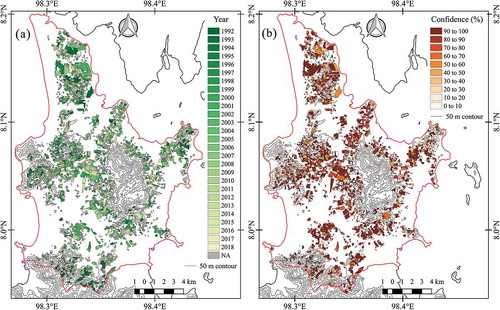
For the highland dataset, 84.7% and 13.4% of training data were corrected and uncorrected classified, respectively. There was only 1.9% of ‘known T_0ʹ highland plantations that were underpredicted. Moreover, there were 22.9% of 1761 plantations and 31.7% of 920 plantations in lowland and highland with ‘unknown T₀’ datasets, respectively, where the actual T₀ could not be determined. It should be noted that this could not lead to an absolute conclusion which all ‘NA’ plantations resulting from the underestimated prediction of the training RP model because there were many more than 30 years old plantations in the study area. The land clearance may occur before the first acquisition date of obtained Landsat image (16 March 1992). The map in Figure 7a shows the dynamic of rubber plantation age resulting from the final prediction. The percentage of nominated T₀ displays in Figure 7b to provide the confidence of the result. There were 1455 out of 3225 (45.1%) plantations that have T₀ predicted with more than 80% confidence.

Figure 7. (a) The map of predicted age of rubber plantations in the study area, and (b) the map of result’s confidence by the percentage of nominated T_0.

4.4. Accuracy assessment

In this study, we conducted an accuracy assessment at two stages. The first assessment was performed when we trained the model using a modelling dataset. Accuracy of the classification was achieved as high as 84.4% and 84.7% for lowland and highland datasets, respectively, during RP modelling. After the simple ensemble method, which based on the percentage of under-condition aggregated result selection and the error analysis, the validation was conducted to assess the accuracy of the predicted establishment year map. Predicted and observed establishment year of rubber plantations with 645 validated ROIs is presented in Figure 8. The scatterplot of predicted and observed the establishment year with different colour shades and sizes of dots is illustrated in Figure 8a. The bigger and black dots indicate a high density of plantations that have the same observed and predicted establishment year and placed along with the 1:1 line. The year with the highest plantation density (47 plots) was in 1992. The ‘NA’ label shows the number of plantations where the planting year (T₀) could not be determined. There were 22 plantations (3.4%) of all validated ROI plantations that under-fitted prediction. Figure 8b illustrates the mean predicted establishment year of rubber plantations against the observed year, which closely distributed along with the 1:1 line. The R² of the linear regression fitted on the mean predicted year is 0.992, and the RMSE is 0.83 years. The young rubber plantations that were planted after 2010 were slightly underpredicted. Further, when we examined particular misclassifications, we found that 40.32% of misclassified plantations (119 plots) were one-year error prediction (±1 year), as shown in Figure 8c. The majority of positive one-year error was the validated ROIs come from the RAOT rubber farmer registration dataset. The main reason for many positive one-year misclassifications is, in fact, many farmers usually start their rubber planting one or two years after the actual approval by RAOT.

Figure 8. Accuracy assessment of the predicted rubber plantation establishment year with 645 validated ROIs: (a) the scatter plot of the predicted against observed establishment year of rubber plantations, (b) error bar plot of mean predicted against observed establishment year of rubber plantations, and (c) the positive and negative errors of predicted establishment year (predicted T₀ – observed T₀). ‘NA’ indicates the number of underprediction in particular years.

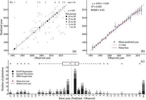
In conjunction with the investigation during error analysis, there was perceptible variability of spectral profile at T₋₁ and T₀ when the land clearance event occurs around the very end of the dry season. In this case, there were many high spectral values scattered from beginning to mid of dry season, and only one or a few low spectral index values which reflect the actual land clearance activity appear around the end of the dry season. Their low values were treated as outliers in the distribution. Thus the median and other summary distribution values remained high at the actual land clearance year, but rather low in the next year, which could be identified as land clearance year by the model. Consequently, there were 17 negative one-year error cases (14.3%). The majority of under-prediction error (‘NA’) was found in the validated ROIs dataset from the interpretation of NDVI and NDMI time series. During the image interpretation, we found that the low NDVI or negative NDMI values inside many plantations extent were observed in the year 1992, which is the first year of Landsat imagery acquisition, and we identified the year 1992 as the starting year of rubber cultivation. However, there could be lower NDVI and NDMI values, which were the actual time of land clearance in a few years before the year 1992. Despite various predicted year errors, the average and the median of error years were −0.66 and 1 years, respectively.

4.5. Uncertainties of predicting rubber plantation establishment year

4.5.1. Availability and accessibility of cloud-free satellite imagery

Cloud-free satellite images were essential for mapping rubber plantation age (Chen et al. 2018a). Although the Landsat images are available every 16 days, Landsat Level-2 SR images acquired during the dry season only be used to avoid images with a high percentage of cloud cover. Since we selected only images that contain less than 20% of cloud cover over our small tropical study area, there were still the presence of cloud cover and some degree on thin cloud contamination in spectral signal in tropical regions during the summer period (Watmough, Atkinson, and Hutton 2011; Chen et al. 2018a). Thus, a few images utilized in some of the dry seasons and the subpixel could contamination substantially affect the distribution of extracted spectral index values, which caused a high variation of inter-annual spectral profiles.

Moreover, the accuracy of the original LULC data is uncertain, given that it was up-dated using other available data sources. There was a limitation for cross-validation of data from Google Earth^TM and RAOT. Google Earth^TM historical imagery over the study area available from 2002, but there were long intervals of accessible images during the early period of image availability. The farmer registration records from RAOT were first recorded in the year 2013, and it accounts for only 3.8% of all plantations. Many pristine rubber tree areas (over 25 years tree) in the original LULC data were used without updating, especially the highland plantations. The accuracy of the visually observed year of rubber planting from satellite and aerial image time series was critical because the incorrect outcomes can affect the performance of the supervised ML algorithm. The predictive model will learn to form continuous or discrete conditions, either in sequent or nested, from the complex features against the known outcome values. The training and validating more accurate data from the ground survey, e.g., intensive plantation owners interviewing or estimating from the length of the tapping line, may improve the predicting accuracy, but high cost and time consuming is the trade-off.

4.5.2. Variability of spectral index profiles

Not only the limited number of obtained images in each dry season that varies inter-annual spectral profiles but also the average of pixel values over the small plantations and their narrow shape could bias the depicted plantation spectral signature, due to the low spatial resolution of Landsat imagery and mixed pixels (Hsien, Lee, and Chen 2001; Choodarathnakara, Kumar, and Patil 2012). The smaller the plantation, the higher the ‘boundary effects’ expected. We found that the predictions made of larger plantations were more accurate than smaller plantations, and ‘boundary effects’ are much reduced.

The deciduous phase of the para rubber trees in the study area is between December and March. It also caused high variability of the VIs values since the partial or completed defoliation of rubber trees is strongly associated with the location of the plantation. The highland rubber trees in the study area are more sensitive to drought than the lowland. Although, the yearly NDVI trend of highland plantations was higher than lowland plantations by average. There was a notable variability of NDVI values in highland plantations where some of low NDVI value caused unbalanced dispersion, as shown in Figure 5. The range from the median to lowest values (or lower whisker) of boxplot was longer than the rang between median and highest values. However, not all highland plantations have a defoliation process, which depends on their location and topographic properties, e.g., slope and contour. Even though in the same plantation extent, rubber trees found in the narrow valley or along the small creek barely have a leaf-off stage. The degree of rubber tree defoliation in the study area strongly associated with the local weather and seasonal variation, as well as the rubber tree species, which have been bred for various drought tolerance and soil properties. This annual variability of spectral index values is the main reasons why the predictors were generated from different significant summary distribution values (e.g., median, Q₁, or Q₃) instead of only minimum or maximum values within the planting year of a rubber tree, and the lowland and highland plantations should be modelled independently.

Moreover, the rubber intercroppedintercropped system is also one of the expressively affected factors. There was a certain degree of distinction between spectral values in monoculture and intercropped plantations during the non-production period of rubber tree growing (first five years), as resulted in Table 1. According to LULC data, more than 90% intercrop in the study area is pineapple. The farmers usually plant unseasonal pineapple between the rubber trees row at the same time of rubber planting and harvest one and a half or two years after that. Two or three pineapple cultivating seasons could be found in many intercropped plantations before the rubber trees have developed a full cover canopy, and this could vary the VIs values between two to five years (T₊₂ to T₊₅) after rubber planting (T₀). Although our approach using distribution properties could minimize the variation of spectral indices, there was still high variability of spectral indices to be modelled by the RP algorithm. The huge advantage of using the RP model is the concept of developing classifiers, as same as other ML algorithms, from a set of training data that contain high-quality information representing the solid structure or pattern of data to be classified. The algorithm will try to explore all the observed features (predictors) and will statistically find the appropriate predictive features to categorize the observation against the known outcome. As a result, shown in Figure 6 (c – f), none of the top five critical predictors used to train RP classifier was created from the summary distribution values at T₊₂ to T₊₅ for lowland dataset, whereas the slope between the median value at T₀ and T₅ was one of the top five critical predictors in the highland dataset. These results imply that modelling the annual green-up trend of rubber plantations that have a massive effect from the intercropped system, as well as a heterogeneous mixture (Li and Fox 2011; Li, Zhang, and Feng 2015), may not be the promising approach. Focusing on the rapid breakdown of vegetation cover that could provide more quality information for training RP classifier since the significant predictors (different, ratio and slope) were derived from summary distribution values at T₋₂, T₋₁, and T₀ in both lowland and highland datasets. Different ML algorithms may not produce the same result due to their underline algorithm. However, in the ML paradigm, the training sample size had more substantial impact on classification accuracy than the algorithm used. Thus, a sufficient training sample for each class (location and agricultural system in this study) and its quality are the key issues and should be a priority in implementing an ML-based classification (Maxwell, Warner, and Fang 2018).

From the error analysis, we also found that the VIs profiles from the pre-conversion land cover (Chen et al. 2018a) which the existing plantations have been converted from other croplands such as rice paddy field, fruit and vegetable orchards, were dissimilar to the re-cultivating rubber plantations or the newly established plantation on the pristine dense evergreen forests. The VIs before the year of land clearance (T₀) may not appear as high as it should be, and thus the greenness breakpoint in the penological profile may not be recognized by the training model. As mention above, the model mostly uses the predictors derived from the NDVI distribution properties at T₋₂ and T₋₁. Therefore, this pre-conversion land cover substantially contributes to the underestimated predictions. We found 12 sample pre-paddy field lowland plantations during the obtaining sample ROI from Google Earth^TM HHR imagery, and they were all misclassified as ‘NA’. If there were a significant number of pre-conversion plantation cases in the training dataset, the RP algorithm might statistically distinguish this yearly spectral index pattern instead appear as a noise.

4.5.3. Reclusive partitioning algorithms

The result from the training RP algorithm was straightforward and closely mirrored human decision-making as the hierarchical conditions were formed and illustrated in the decision tree model. Figure 9(a, b) demonstrated the examples of the decision trees of RP algorithm when using CP as 0.05 and 0.03, respectively, in lowland data model training. The root-level predictor was ‘ndvi.ratio.MEDt0.Q3tn1ʹ. Only this predictor with the condition as ‘< 1.337ʹ, the model correctly classified 6718 of ‘0:No’ outcomes and misclassified 77 of ‘1:Yes’ as the ‘0:No’ outcomes. Accordingly, the model with the second predictors can accurately classify 145 of ‘1:Yes’ outcomes using the nested condition: ‘ndvi.ratio.MEDt0.Q3tn1ʹ ≥ 1.337, and then ‘ndvi.diff.MINt0.MAXtn2ʹ < −0.3118.

Figure 9. Comparison of example decision trees from RP model training using complexity parameter as (a) 0.05 and (b) 0.03.

The model with smaller CP produced more splitting of the tree. Therefore more nested conditions were introduced, and more accuracy was accomplished. Different nominated predictors and their values to build a good representation depend on different assumptions about the training data. This advantage contributes to the ability of training RP models to denote different structures of data whenever there is a specific mapping pattern of input and output variables. In this study, the predictors were generated based upon the pattern of the inter-annual NDVI profile between two years before to six years after the year that the event of land preparation for rubber planting was found, as shown in Figure 5. There were many methods to create the predictors from the spectral index time series that characterize the event of the loss of vegetation cover and the increase of canopy cover from rubber plantings as they grow to maturity (Chen et al. 2018a). Finding the optimum combination of informative predictors is a universal principle that underlies all supervised ML algorithms for predictive modelling. We demonstrated that only the use of the more straightforward methods to create predictors from only the NDVI profile could accomplish acceptable prediction accuracy. Moreover, instructive predictors could be used to improve the accuracy, but more importantly, eliminating the variation of inter-annual spectral index trend caused by the drawback issues specified in Section 4.6.2 is promising but most likely need more extensive datasets than were available in the present study. Alternatively, separately modelling different groups of plantations such as by elevation and pre-conversion, to reduce profile variation could also increase prediction accuracy, as we demonstrated in this study. Moreover, including potential information, e.g., elevation and slope of plantations into the set of predictors and leave the RP algorithm to decide based on the given set of predictive data.

Unlike the threshold-based approaches (Kou et al. 2015; Beckschäfer 2017; Chen et al. 2018a) in pixel-based image classification to identify the age of rubber plantations, the RP algorithm does not require the global references. This supervised tree-based algorithm learns and creates the discrete function that best maps predictors to an outcome from the structure of given training data against the known outcomes. The form of the function being learned depends on the complicated relationship between the outcome and predictors, whether it is linear or nonlinear (regression tree or classification tree). Moreover, the presented approach of forming predictors from summary distribution values that represent characteristic of rapid greenness breakdown and gradually change of vegetation cover during rubber tree closing-canopy period allows the RP algorithm to numerically explore the various data structure of predictors corresponding to predicted outcomes not just only the values of the global thresholds. With the difficulty of acquiring satellite images at the precise time of completed land clearance, different land preparing practices of individual smallholder, size and location of plantation, different rubber-based agricultural system, and local climate conditions, global references such as sub-zero NDMI value (Beckschäfer 2017; Chen et al. 2018a) and modelling rubber tree growth (Chen et al. 2018b) may not be practicable in such inevitable variability of spectral index values and their annual profiles.

5. Conclusion

We investigated the potential of using tree-based ML techniques to identify the establishment year of para rubber plantations in Thalang District, Phuket Province, Southern of Thailand from multitemporal Landsat cross-sensor images and secondary LULC data. The supervised RP classifier was learned from the training dataset, which extracted and derived from 129 Landsat images. The specific predictors in training data were the combination of the difference, ratio, and slope of spectral indices distribution properties at different years between two years (T₋₂) before and six years after (T₊₆) of a particular year in 27 years inter-annual spectral index profiles. The presenting approach of generating predictors and the simple RP algorithm achieved mapping rubber plantation at an annual scale with RMSE 0.83 years. The study also demonstrated that

1. Among four multitemporal Landsat-derived spectral indices (i.e., NDVI, EVI, SAVI, and NDMI), only the inter-annual NDVI profile was a significant candidate as been repeatedly used in forming predictive RP model.

2. The characteristics of rapid greenness breakdown period, either the slope or the change of NDVI values between one or two years before (T₋₁ or T₋₂) and the year of land clearance occur (T₀), exhibited to be the potential parameters for identifying rubber plantation age.

3. The tree-based RP algorithm can learn from the sufficient and good quality of sample training dataset to form a set of linear or discrete functions used for high accurate predicting unknown outcomes from the new sets of predictors. Thus, no pre-defined global thresholds or pre-developing models were required.

Despite many limitations of acquired satellite-based data, the presented approach provided an acceptable result and has high potential to overcome the acquisition of rubber plantations age with field observation, which is time-consuming, laborious and expensive (Chen et al. 2012a; Beckschäfer 2017), yielding the needed information for the national precision agriculture database.

Contribution

Natthaphon Somching graduated with B.Sc degree in environmental geoinformatics in 2014 from Faculty of Technology and Environment, Prince of Songkla University and has continued his higher education of M.Sc. in Environmental Management Technology. His master thesis involved utilizing GIS and RS technologies in agricultural land use and environmental management.

Noppachai Wongsai was a senior lecturer at Prince of Songkla University (PSU), Phuket campus. He received his Ph.D. degree in Research Methodology. Since his backgrounds are computer engineering (B.Eng.) and IT (M.Sc.), his main research interests aim to data sciences in geoinformatics for environment and climate.

Sangdao Wongsai is currently an assistant professor and a lecturer at Thammasat University. She received her Ph.D. degrees in applied statistics from Macquarie University in Sydney, Australia. She teaches spatial statistics, geoinformatics research methodology, and GIS applications to graduate and undergraduate courses. Her main research interests include data sciences in the environment, ecology, energy, land and water, and tourism management. She is a member of International Statistic Institute (ISI).

Werapong Koedsin was received the Ph.D. (Survey Engineering) degrees from Chulalongkorn University, Thailand, in 2013. He is currently a researcher with the Tropical Plants Biology Research Unit, Faculty of Technology and Environment, Prince of Songkla University, Thailand. His research interests include Hyperspectral Remote Sensing, Vegetation dynamics, Land Surface Phenology, and vegetation biophysical variable estimating.

Acknowledgements

This research had been supported by the Faculty of Technology and Environment, Prince of Songkla University, and Thammasat University Research Unit in Data Learning. We wish to thank the Land Development Department (LDD), Thailand’s Ministry of Agriculture and Cooperatives and Rubber Authority of Thailand (RAOT), Phuket office for their data support. We would like to gratefully and sincerely thank Asst. Prof. Dr. Chanida Suwanprasit and Assoc. Prof. Dr. Raymond J. Ritchie for their useful guidance and continual encouragement.

Disclosure statement

No potential conflict of interest was reported by the authors.

Additional information

Funding

This work was supported by the Faculty of Technology and Environment, Prince of Songkla University [Research Assistant Scholarship].

References

- Bannach-Brown, A., P. Przybyła, J. Thomas, A. S. C. Rice, S. Ananiadou, J. Liao, and M. R. Macleod. 2019. “Machine Learning Algorithms for Systematic Review: Reducing Workload in a Preclinical Review of Animal Studies and Reducing Human Screening Error.” Systematic Reviews 8 (1): 23. doi:10.1186/s13643-019-0942-7.
- Beckschäfer, P. 2017. “Obtaining Rubber Plantation Age Information from Very Dense Landsat TM & ETM + Time Series Data and Pixel-Based Image Compositing.” Remote Sensing of Environment 196: 89–100. doi:10.1016/j.rse.2017.04.003.
- Breiman, L., J. H. Friedman, R. A. Olshen, and C. J. Stone. 1984. Classification and Regression Trees. Pacific Grove, California: Wadsworth.
- Chaiyarat, N. 2007. “Guidelines for Development Tourism Area on the Tsunami Disaster Area: A Case Study of Kamala Beach, Amphoe Kathu, Phuket Province.” Journal of Architectural/Planning Research and Studies 5 (2): 53–76.
- Chantuma, P., R. Lacote, A. Leconte, and E. Gohet. 2011. “An Innovative Tapping System, the Double Cut Alternative, to Improve the Yield of Hevea Brasiliensis in Thai Rubber Plantations.” Field Crops Research 121 (3): 416–422. doi:10.1016/j.fcr.2011.01.013.
- Chen, B., J. Cao, J. Wang, Z. Wu, Z. Tao, J. Chen, C. Yang, et al. 2012a. “Estimation of Rubber Stand Age in Typhoon and Chilling Injury Afflicted Area with Landsat TM Data: A Case Study in Hainan Island, China.” Forest Ecology and Management 274:222–230. doi:10.1016/j.foreco.2012.01.033.
- Chen, B., X. Guishui, W. Jikun, W. Zhixiang, and C. Jianhua. 2012b. “Estimation of Rubber Stand Age Using Statistical and Artificial Neural Network Approaches with Landsat TM Data.” Chinese Journal of Tropical Crops 1: 182–188.
- Chen, B., X. Xiao, Z. Wu, T. Yun, W. Kou, H. Ye, Q. Lin, et al. 2018a. “Identifying Establishment Year and Pre-Conversion Land Cover of Rubber Plantations on Hainan Island, China Using Landsat Data during 1987-2015.” Remote Sensing 10 (8): 1240. doi:10.3390/rs10081240.
- Chen, G., J.-C. Thill, S. Anantsuksomsri, N. Tontisirin, and R. Tao. 2018b. “Stand Age Estimation of Rubber (Hevea Brasiliensis) Plantations Using an Integrated Pixel- and Object-based Tree Growth Model and Annual Landsat Time Series.” ISPRS Journal of Photogrammetry and Remote Sensing 144: 94–104. doi:10.1016/j.isprsjprs.2018.07.003.
- Choodarathnakara, A. L., A. Kumar, and G. Patil. 2012. “Mixed Pixels: A Challenge in Remote Sensing Data Classification for Improving Performance.” Journal of Advances in Computer Engineering and Technology 1 (9): 261–271.
- Dibs, H., M. O. Idrees, and G. B. A. Alsalhin. 2017. “Hierarchical Classification Approach for Mapping Rubber Tree Growth Using Per-Pixel and Object-Oriented Classifiers with SPOT-5 Imagery.” The Egyptian Journal of Remote Sensing and Space Sciences 20 (1): 21–30. doi:10.1016/j.ejrs.2017.01.004.
- Ding, L., and B.-H. Sheng. 2010. “Error Analysis of Classifiers in Machine Learning.” In 3rd International Congress on Image and Signal Processing. Yantai, China. doi:10.1109/CISP.2010.5646324.
- Dong, J., X. Xiao, B. Chen, N. Torbick, C. Jin, G. Zhang, and C. Biradar. 2013. “Mapping Deciduous Rubber Plantations through Integration of PALSAR and Multi-temporal Landsat Imagery.” Remote Sensing of Environment 134: 392–402. doi:10.1016/j.rse.2013.03.014.
- Grogan, K., D. Pflugmacher, P. Hostert, R. Kennedy, and R. Fensholt. 2015. “Cross-Border Forest Disturbance and the Role of Natural Rubber in Mainland Southeast Asia Using Annual Landsat Time Series.” Remote Sensing of Environment 169: 438–453. doi:10.1016/j.res.2015.03.001.
- Hsien, P.-F., L. C. Lee, and N.-Y. Chen. 2001. “Effect of Spatial Resolution on Classification Errors of Pure and Mixed Pixels in Remote Sensing.” IEEE Transactions on Geoscience and Remote Sensing 39 (12): 2657–2663. doi:10.1109/36.975000.
- Izenman, A. J. 2013. “Recursive Partitioning and Tree-Based Methods.”Chap. 9 in Modern Multivariate Statistical Techniques, Springer, 281-314. New York, NY: Springer Texts in Statistics. doi:10.1007/978-0-387-78189-1_9.
- Koedsin, W., and A. Huete. 2015. “Mapping Rubber Tree Stand Age Using Pléiades Satellite Imagery: A Case Study in Thalang District, Phuket, Thailand.” Engineering Journal 19 (4): 45–56. doi:10.4186/ej.2015.19.4.45.
- Koedsin, W., and K. Yasen. 2016. “Estimating Leaf Area Index of Rubber Tree Plantation Using Worldview-2 Imagery.” Journal of Life Sciences and Technologies 4 (1): 1–6. doi:10.18178/jolst.4.1.1-6.
- Kou, W., J. Dong, X. Xiao, A. J. Hernandez, Y. Qin, G. Zhang, B. Chen, N. Lu, and R. Doughty. 2018. “Expansion Dynamics of Deciduous Rubber Plantations in Xishuangbanna, China during 2000–2010.” GIScience & Remote Sensing 55 (6): 905–925. doi:10.1080/15481603.2018.1466441.
- Kou, W., X. Xiao, J. Dong, S. Gan, D. Zhai, G. Zhang, Y. Qin, and L. Li. 2015. “Mapping Deciduous Rubber Plantation Areas and Stand Ages with PALSAR and Landsat Images.” Remote Sensing 7 (1): 1048–1073. doi:10.3390/rs70101048.
- Li, P., J. Zhang, and Z. Feng. 2015. “Mapping Rubber Tree Plantations Using A Landsat-based Phenological Algorithm in Xishuangbanna, Southwest China.” Remote Sensing Letters 6 (1): 49–58. doi:10.1080/2150704X.2014.996678.
- Li, Z., and J. M. Fox. 2011. “Rubber Tree Distribution Mapping in Northeast Thailand.” International Journal of Geosciences 2 (4): 573–584. doi:10.4236/ijg.2011.24060.
- Li, Z., and J. M. Fox. 2012. “Mapping Rubber Tree Growth in Mainland Southeast Asia Using Time-series MODIS 250 m NDVI and Statistical Data.” Applied Geography 32 (2): 420–432. doi:10.1016/j.apgeog.2011.06.018.
- Masek, J. G., E. F. Vermote, N. E. Saleous, R. Wolfe, F. G. Hall, K. F. Huemmrich, F. Gao, et al. 2006. “A Landsat Surface Reflectance Dataset for North America, 1990–2000.” IEEE Geoscience and Remote Sensing Society 3 (1): 68–72. doi:10.1109/LGRS.2005.857030.
- Maxwell, A. E., T. A. Warner, and F. Fang. 2018. “Implementation of Machine-learning Classification in Remote Sensing: An Applied Review.” International Journal of Remote Sensing 39 (9): 2784–2817. doi:10.1080/01431161.2018.1433343.
- Polikar, R. 2006. “Ensemble Based Systems in Decision Making.” IEEE Circuits and Systems Magazine 6 (3): 21–45. doi:10.1109/MCAS.2006.1688199.
- Powers, D. M. W. 2011. “Evaluation: From Precision, Recall and F-Measure to ROC, Informedness, Markedness & Correlation.” Journal of Machine Learning Technologies 2 (1): 37–63.
- Prommee, V., T. Phomchai, N. Laykhaviphat, N. Chanrueang, K. Theerawattanasuk, P. Chantuma, P. Suchatkul, et al. 2018. Academic Information of Para Rubber (2018). 1st ed. Bangkok: RAOT.
- Putklang, W., C. Mongkolsawat, and R. Suwanwerakamtorn. 2019. “Object-Based Image Analysis Applied for Different Stages of Rubber Plantations Mapping Using THAICHOTE Satellite Data.” Journal of Theoretical and Applied Information Technology 97 (6): 1720–1746.
- QGIS Development Team. 2018. “QGIS Geographic Information System. Open Source Geospatial Foundation Project.” Accessed 25 December 2018. http://qgis.osgeo.org
- Razak, J. A. A., A. R. M. Shariff, N. Ahmad, and M. I. Sameen. 2018. “Mapping Rubber Trees Based on Phenological Analysis of Landsat Time Series Datasets.” Geocarto International 33: 627–650. doi:10.1080/10106049.2017.1289559.
- Rokach, L. 2010. “Ensemble-Based Classifiers.” Artificial Intelligence Review 33 (1–2): 1–39. doi:10.1007/s10462-009-9124-7.
- Simien, A., and E. Penot. 2011. “Current Evolution of Smallholder Rubber-Based Farming Systems in Southern Thailand.” Journal of Sustainable Forestry 30 (3): 247–260. doi:10.1080/10549811.2011.530936.
- Suratman, M. N., G. Q. Bull, D. G. Leckie, V. M. Lemay, P. L. Marshall, and M. R. Mispan. 2004. “Prediction Models for Estimation the Area, Volume, and Age of Rubber (Hevea Brasiliensis) Plantation in Malaysia Using Landsat TM Data.” The International Forestry Review 6 (1): 1–12. doi:10.1505/ifor.6.1.1.32055.
- Tang, F., and H. Ishwaran. 2017. “Random Forest Missing Data Algorithms.” Statistical Analysis and Data Mining: The ASA Data Science Journal 10 (6): 363–377. doi:10.1002/sam.11348.
- Thenkabail, P. S. 2003. “Biophysical and Yield Information for Precision Farming from Near-real-time and Historical Landsat TM Images.” International Journal of Remote Sensing 24 (14): 2879–2904. doi:10.1080/01431160710155974.
- Therneau, T., B. Atkinson, and B. Ripley. 2018. “Recursive Partitioning and Regression Trees, R ‘Rpart’ Package Documentation, Version 4.1-13.” February 23. Accessed 13 December 2018. https://cran.r-project.org/web/packages/rpart/rpart.pdf
- Trisasongko, B. H. 2017. “Mapping Stand Age of Rubber Plantation Using ALOS-2 Polarimetric SAR Data.” European Journal of Remote Sensing 50 (1): 64–76. doi:10.1080/22797254.2017.1274569.
- Vermote, E., C. Justice, M. Claverie, and B. Franch. 2016. “Preliminary Analysis of the Performance of the Landsat 8/OLI Land Surface Reflectance Product.” Remote Sensing of Environment 185: 46–56. doi:10.1016/j.rse.2016.04.008.
- Watmough, G. R., P. M. Atkinson, and C. W. Hutton. 2011. “A Combined Spectral and Object-Based Approach to Transparent Cloud Removal in an Operational Setting for Landsat ETM+.” International Journal of Applied Earth Observation and Geoinformation 13 (2): 220–227. doi:10.1016/j.jag.2010.11.006.
- Xiao, C., P. Li, Z. Feng, Z. You, L. Jiang, and K. Boudmyxay. 2020. “Is the Phenology-based Algorithm for Mapping Deciduous Rubber Plantations Applicable in an Emerging Region of Northern Laos?” Advances in Space Research 65 (1): 446–457. doi:10.1016/j.asr.2019.09.022.
- Ye, S., J. Rogan, and F. Sangermano. 2018. “Monitoring Rubber Plantation Expansion Using Landsat Data Time Series and a Shapelet-based Approach.” ISPRS Journal of Photogrammetry and Remote Sensing 136: 134–143. doi:10.1016/j.isprsjprs.2018.01.002.
- Zhou, Z.-H. 2012. Ensemble Methods: Foundations and Algorithms. 1st ed. Boca Raton, FL: Chapman & Hall/CRC Press, Taylor & Francis Group.