Assessment of linear relationships between TanDEM-X coherence and canopy height as well as aboveground biomass in tropical forests

ABSTRACT

Information about the forest structure attributes like canopy height and aboveground biomass (AGB) are crucial for forest monitoring systems and in the assessment of the global carbon cycle. The globally available TerraSAR-X add-on for Digital Elevation Measurement (TanDEM-X) data are a potential data source for estimating canopy height and AGB. Several empirical and semi-empirical investigations have indicated a linear relationship between X-band coherence and canopy height as well as AGB. The generality of this relationship is to date underexplored. In this study, the volume coherence of bistatic TanDEM-X acquisitions was retrieved and linearly related to canopy height and AGB in different tropical study areas to assess the generality of their relationship. Airborne light detection and ranging (LiDAR) data were also used to complement the estimation of canopy height and AGB with the X-band volume coherence. The results indicated that the linear function provides a statistically significant fit to the observed relationship between coherence and canopy height as well as AGB. The estimation of canopy height with this linear relationship resulted in a coefficient of determination R² of 0.72 and a root mean square error (RMSE) of 6.4 m (15.7%), where the AGB estimation had a decreased accuracy with an R² of 0.59 and RMSE of 88.2 t ha⁻¹ (21%). The estimation where the LiDAR (light detection and ranging)-based AGB relationship and coherence was combined revealed generally similar accuracies compared to the coherence alone. This confirms that the TanDEM-X coherence can support the consistent estimation of canopy height and AGB, where it provides as a minimum a source for a stratification to assess the spatial distribution of qualitative AGB classes.

1. Introduction

Forests are highly relevant to the global carbon cycle and climate change, where they act as sinks when growing, sources when disturbed and as stable pool when undisturbed for CO₂ (GCOS 2015). The estimation of forest structural properties like aboveground biomass (AGB) for retrieving information about its spatial distribution and change over time is essential to understand and quantify the global carbon balance (Pan et al. 2011). The combination of field measurements and remote sensing seems particularly useful for forest monitoring and the estimation of the structural properties of forests on a large spatial scale (Gibbs et al. 2007). The potential of synthetic aperture radar (SAR) data for forest monitoring applications has long been recognized. Low frequencies like L- and P-band are generally considered to have more potential than high frequencies like X- and C-band in forestry applications, such as in estimating AGB due to their higher penetration capability (Le Toan et al. 1992; Imhoff 1995; Castro, Sanchez-Azofeifa, and Rivard 2003; Schlund and Davidson 2018). However, the potential of high-frequency SAR systems for monitoring forests and estimating their height and AGB has also been demonstrated, in which their interferometric information was found to be particularly useful (Solberg et al. 2010; Treuhaft et al. 2015; Schlund et al. 2015, 2016; Olesk et al. 2016; Schlund et al. 2019). Other key technologies for monitoring forest and estimating their structural attributes are passive microwave (Liu et al. 2015) and LiDAR (light detection and ranging) sensors (Lefsky et al. 2005; Asner 2009; Hu et al. 2016) as well as the combination of different sensors (Saatchi et al. 2011; Baccini et al. 2012; Hu et al. 2016).

LiDAR data have achieved high accuracies in the estimation of forest canopy height and AGB, but is normally limited in its spatial coverage and thus has to be integrated into a sampling scheme to receive a consistently wide coverage (Asner 2009; Qi et al. 2019; Schlund, Erasmi, and Scipal 2020). In contrast, the TerraSAR-X add-on for Digital Elevation Measurement (TanDEM-X) mission provides interferometric SAR (InSAR) data consistently on global scale, where the interferometric coherence was used to estimate canopy height and AGB in different case studies (Kugler et al. 2014; Treuhaft et al. 2015; Schlund et al. 2015; Chen, Cloude, and Goodenough 2016; Joetzjer et al. 2017; Chen et al. 2018; Olesk et al. 2016; Schlund et al. 2019). These studies evaluated the relationship at each study area individually, where the empirical basis of the relationship between TanDEM-X coherence and canopy height as well as AGB was not rigorously assessed. Consequently, the validity and generality of the found relationships are to date underexplored. A generic relationship across biomes and different forests between coherence and canopy height as well as AGB would support the globally consistent estimation of these variables. Moreover, it could improve the understanding of the effect of different forest structures even though the generic relationship might result in lower accuracies compared to a locally calibrated model (Knapp et al. 2020).

A linear relationship has been frequently used to estimate AGB as well as canopy height with TanDEM-X coherence (Treuhaft et al. 2015; Schlund et al. 2015; Olesk et al. 2016; Schlund et al. 2019). This is based on the fact that the Random Volume over Ground (RVoG) model must be simplified for TanDEM-X single-polarization acquisitions, whereby the RVoG or derivations of it are commonly used to estimate canopy height with polarimetric interferometric SAR data (PolInSAR) (Kugler et al. 2014; Khati, Singh, and Ferro-Famil 2017). In most studies, the simplifications rely on the assumption that the extinction of the TanDEM-X data is zero and the X-band wave will not penetrate to the ground, which results in a sinc model (Chen, Cloude, and Goodenough 2016; Olesk et al. 2016; Schlund et al. 2019). Furthermore, it is known that the models perform best if the forest height is in the range or smaller than the height of ambiguity (HoA). This also means that a linear function can be used to approximate the sinc function. Consequently, a linear model could be established between TanDEM-X coherence and canopy height, where previous studies have found that this linear relationship performed similarly to the sinc model (Olesk et al. 2016; Schlund et al. 2019). A linear relationship between AGB and canopy height models (CHM) from TanDEM-X or LiDAR data has been found in other studies (Solberg et al. 2010, 2013; Schlund et al. 2016; Solberg et al. 2017; Schlund, Erasmi, and Scipal 2020). It can be argued that the canopy heights are a plot level aggregated metric (Asner and Mascaro 2014), which is affected by the height and the canopy density, where the AGB is determined by the product of these two properties (Treuhaft and Siqueira 2004; Solberg et al. 2013). This is in contrast to allometry based on individual trees and a linear relationship was considered appropriate (Solberg et al. 2013). It can be assumed that a linear relationship between interferometric coherence and canopy height as well as between canopy height and AGB will result in a linear relationship between interferometric coherence and AGB, which has been confirmed in different individual areas (Treuhaft et al. 2015; Schlund et al. 2015).

The objective of this study is to assess the linear relationship of interferometric coherence and canopy height as well as AGB in different tropical forests on three continents to empirically confirm the validity and generality of these relationships. Having established the generality of the linear relationship between coherence and canopy height as well as AGB, it is then used to estimate both quantities. It is worth noting that empirical functions are necessary to provide reliable results in the estimation of canopy height and AGB with TanDEM-X single-polarized coherence (Schlund et al. 2015; Chen, Cloude, and Goodenough 2016; Olesk et al. 2016; Schlund et al. 2019). This requires a calibration (i.e. training) of the empirical linear functions. However, once a general relationship between different quantities has been established, the calibration of the empirical functions can be supported with external data sources like LiDAR data. Therefore, in this study, it has been assessed if a linear relationship between LiDAR-based canopy height and AGB can be also used to support the calibration of the empirical function between TanDEM-X coherence and AGB or canopy height. This could be a way forward combining data from TanDEM-X and airborne LiDAR data or even spaceborne missions like GEDI (Qi and Dubayah 2016; Qi et al. 2019; Schlund, Erasmi, and Scipal 2020). This would enable the combined use of the different sensor systems such as LiDAR and InSAR, which would support a spatially and temporally consistent estimation of canopy height and AGB. Such an estimation could be used, at a minimum, to provide information about the canopy height and AGB distribution, but it could be also assimilated into dynamic ecosystem and vegetation models (Joetzjer et al. 2017; Yang et al. 2020).

2. Data

2.1. Study areas and in situ data

The study areas are distributed over three continents covering South-American, African, and Asian tropical forests. Furthermore, the study was conducted in different types of tropical forests, which included the transition from savannah to mature tropical forests as well as tropical peat swamp forest.

Three study areas were in Gabon, namely Lopé, Mondah and Rabi. Lopé is a protected forest area about 250 km east of Libreville. This area included the transition from savannah to mature tropical forest resulting in a high structural diversity (Labriere et al. 2018; Silva et al. 2018). In contrast to Lopé, in Mondah parts of the forests were disturbed or deforested, whereas others remained pristine (Walters et al. 2016; Labriere et al. 2018). This study area is a coastal area about 25 km northwest of Libreville. Rabi, about 260 km south of Libreville, is a lowland tropical forest. It is partially protected similar to Mondah, but oil drilling is also carried out in this area. However, parts of the forest were kept intact to preserve the forest, which was true for the forest plots (Labriere et al. 2018). Paracou is a study area south of Sinnamary in French Guiana, South America, which is also mainly covered by tropical lowland forest (Dubois-Fernandez et al. 2012; Schlund, Erasmi, and Scipal 2020). The Mawas study area is located about 60 km east of Palangkaraya, Central Kalimantan, Indonesia. This is a tropical peat swamp forest, which is under protection as conservation area (Schlund et al. 2015).

Forest inventories were conducted for all study areas, by which data from a total of 84 plots were available for this study (Table 1). The size of the plots varied from 0.1 ha in Mawas to 6.25 ha (n= 15) and 25 ha (n= 1) in Paracou (Schlund et al. 2015; Labriere et al. 2018). The size of the plots in Gabon was generally 1 ha, whereas three plots of young colonizing forest in Lopé were 0.5 ha Labriere et al. (2018). The tree measurement protocols were generally similar where the tree height and diameter at breast height (DBH) of trees when more than 10 cm were measured. The height was measured from a sample of trees in French Guiana and the African areas, where Michaelis–Menten models were used to predict the tree height from DBH (Molto et al. 2014; Labriere et al. 2018). Trees with more than 5 cm DBH were measured in Savannah and young colonizing forest plots in Lopé, which was the only exception based on the fact that these plots mainly consisted of small trees contributing substantially to the AGB (Labriere et al. 2018). The same non-linear allometric equation was applied in all study areas to estimate the AGB for each tree, where the DBH (cm), tree height (m), and oven-dry wood density (gcm⁻³) was used (Chave et al. 2014). The AGB for each tree was summed and normalized to a 1 ha unit area resulting in a plot-based AGB in t ha⁻¹. Density values were extracted from the Global Wood Density Database (Chave et al. 2009). More information and the data can be obtained from the Forest Observation System (FOS) (Schepaschenko et al. 2019a, 2019b).

Table 1. Study areas and average CHM (with range in brackets) and AGB (with range in brackets) of available forest plots (n is the number of forest plots used in this study)

Study area	CHM (m)	AGB (t ha^−1)	n	Year of inventory	Year of LiDAR acquisition
Lopé	25.5	218.4
	(1.9 to 42.7)	(0.6 to 404.2)	12	2016	2016
Mawas	18.2	168.6
	(13.3 to 25.1)	(106.4 to 235.7)	16	2014 to 2015	2007
Mondah	19.4	119.7
	(5.0 to 31.3)	(2.3 to 331.8)	15	2016	2016
Paracou	27	319.9
	(24.3 to 30.7)	(257.5 to 485.7)	16	2009	2009
Rabi	32.7	298.2
	(28.0 to 37.7)	(205.2 to 513.9)	25	2010 to 2012	2016

The plot AGB ranged in the different study areas from 0.6 t ha⁻¹ in Lopé to 513.9 t ha⁻¹ in Rabi. In general, the ranges of AGB were relatively similar, whereas the averages of AGB were different between the individual areas. Mondah had the lowest average AGB at 119.7 t ha⁻¹ and Paracou had the highest average AGB of 319.9 t ha⁻¹ (Table 1).

2.2. Remote sensing data

2.2.1. TanDEM-X data

The TanDEM-X mission consists of two X-band SAR satellites flying in close formation, which are able to acquire single-pass interferometric SAR data to create a global digital elevation model (DEM) (Krieger et al. 2007). Both sensors use a phased-array X-band antenna with a carrier frequency of 9.65 GHz (i.e. 3.1 cm wavelength) to transmit and receive the electromagnetic waves (Pitz and Miller 2010).

Only TanDEM-X datasets that had also been utilized in the creation of the TanDEM-X DEM in the respective study areas were used in this study. Consequently, the data were acquired in horizontal polarization (transmit and receive; HH) and StripMap mode resulting in a resolution of about 3 m (Table 2). One sensor acts as transmitter and receiver (monostatic/active) while the other only receives (bistatic/passive) the electromagnetic waves in the bistatic acquisition mode. Spectral filtering in azimuth and range was applied in order to reduce decorrelation due to Doppler centroid shift and the geometric properties of the acquisition, and the data were co-registered and resampled to CoSSC (co-registered single-look slant range complex) data products (Fritz 2012).

Table 2. Summary of TanDEM-X datasets (incidence angle θ and height of ambiguity (HoA) at the centre of the scene)

Study area	Acquisition date	θ (°)	Resolution (m) azimuth × range	HoA (m)	Orbit
Lopé	31 December 2010	46.3	3.3 × 2.4	49.8	Descending
	2 October 2011	46.1	3.3 × 1.6	86.3	Descending
Mawas	21 December 2010	47.7	3.3 × 2.4	51.2	Descending
	21 April 2014	47.7	3.3 × 3.4	72.1	Descending
Mondah	17 November 2017	47.7	3.3 × 2.4	51.3	Descending
	12 March 2018	31.3	3.3 × 3.4	52.4	Descending
Paracou	15 September 2011	36.2	3.3 × 3.0	48.2	Ascending
	5 January 2014	37.1	3.3 × 3.0	66.5	Descending
Rabi	6 May 2011	40.5	3.3 × 2.7	54.0	Descending
	22 January 2013	41.4	3.3 × 2.7	101.7	Descending

The height of ambiguity was about 50 m for all acquisitions. This height of ambiguity was generally used for the global TanDEM-X acquisition because it achieved the best trade-off in terms of interferometric accuracy and sensitivity (Martone et al. 2012). In addition, a height of ambiguity which is approximately similar or higher than the maximum canopy heights resulted in the best results of the canopy height estimation (Schlund et al. 2019). The consistency of the established models was tested in each study area, where the acquisition parameters should be similar. Consequently, two TanDEM-X acquisitions for each study area were selected, which were in line with these conditions. Note that most available acquisitions with this height of ambiguity and that were temporally not too different to in situ and LiDAR data acquisition was acquired in descending orbit direction, while only one acquisition in Paracou was acquired in ascending orbit.

2.2.2. Airborne laser scanning data

Airborne laser scanning (ALS) data acquired with LiDAR sensors were available for all study areas. The ALS data were collected with a small footprint Riegl laser rangefinder in Paracou and Mawas (Dubois-Fernandez et al. 2011; Schlund et al. 2015, 2016). The point clouds were used to retrieve a digital surface model (DSM) and a digital terrain model (DTM) with a 1 m spatial resolution in both areas. A large footprint laser altimeter system, namely NASA’s Land, Vegetation, and Ice Sensor (LVIS), was used to collect full-waveform data with a nominal footprint diameter of 18 m in the African areas (Blair, Rabine, and Hofton 1999). The lowest mode within the waveform was used to detect the ground elevation (DTM), whereas the height at which 98% of the waveform energy occurs in relation to the ground elevation was used to retrieve the surface height (DSM) (Blair, Hofton, and Rabine 2018). The 98% percentile height was used because it proved best when large footprint data from LVIS were compared to a small footprint LiDAR sensor, where both resulted in similar ground and forest heights (Silva et al. 2018). The heights of the LVIS system were gridded to 15 m pixel spacing.

The CHM based on the ALS data with small and large footprint LiDAR sensors was calculated by subtracting pixelwise the DTM from the DSM. The pixels of each CHM within an in situ plot were extracted and averaged to retrieve the average canopy height of each plot. The canopy height in the different study areas ranged from 1.9 m to 42.7 m, where both were found in Lopé. The smallest canopy heights were found on average in Mawas (18.2 m), whereas the largest average canopy heights were found in Rabi (32.7 m) (Table 1).

3. Methods

3.1. Volume coherence estimation

The volume coherence was derived from the TanDEM-X data, where first the interferometric coherence for each TanDEM-X acquisition was estimated. Multi-look processing was applied to obtain a spatial resolution of 12 m. The interferometric coherence is a product of individual coherence contributions, where they can be assumed to be independent (Krieger et al. 2007; Martone et al. 2012, 2018). The ${\gamma }_{\mathrm{S}\mathrm{N}\mathrm{R}}$ and ${\gamma }_{\mathrm{V}\mathrm{o}\mathrm{l}}$ were the main remaining coherence contributions in the used TanDEM-X acquisitions since spectral filtering was applied in the CoSSC generation and the simultaneous acquisitions resulted in negligible temporal decorrelation (Duque et al. 2012; Fritz 2012; Martone et al. 2012). The ${\gamma }_{\mathrm{V}\mathrm{o}\mathrm{l}}$ was finally retrieved from the estimated coherence

(1) ${\gamma }_{\mathrm{V}\mathrm{o}\mathrm{l}}=\frac{\gamma }{{\gamma }_{\mathrm{S}\mathrm{N}\mathrm{R}}}$(1)

The signal-to-noise ratio (SNR) coherence ${\gamma }_{\mathrm{S}\mathrm{N}\mathrm{R}}$ is a function of the SNR of the individual channels

(2) ${\gamma }_{\mathrm{S}\mathrm{N}\mathrm{R}}=\frac{1}{\sqrt{1+{\mathrm{S}\mathrm{N}\mathrm{R}}_1^{-1}}\sqrt{1+{\mathrm{S}\mathrm{N}\mathrm{R}}_2^{-1}}}$(2)

and the SNR for image i can be calculated as

(3) $\mathrm{S}\mathrm{N}{\mathrm{R}}_i=\frac{{\beta }^{0}sin\theta -\mathrm{N}\mathrm{E}\mathrm{S}\mathrm{Z}}{\mathrm{N}\mathrm{E}\mathrm{S}\mathrm{Z}}$(3)

where ${\beta }^0$ means backscattering coefficient, θ means the incidence angle and NESZ means the noise equivalent sigma zero, which describes the noise from the antenna pattern and the antenna’s thermal noise (Martone et al. 2012). The NESZ pattern was available for every TanDEM-X acquisition, which was used to calculate the NESZ for every pixel and channel. This was further utilized to calculate the SNR and SNR coherence ${\gamma }_{\mathrm{S}\mathrm{N}\mathrm{R}}$ for every pixel.

3.2. Linear relationships between volume coherence and canopy height as well as aboveground biomass

The linear relationship between volume coherence and canopy height could be supported by the fact that the frequently used RVoG (Random Volume over Ground) is most appropriate when the maximum canopy height equals the height of ambiguity, and thus the canopy height $h_{\mathrm{V}}$ should be normalized with the height of ambiguity (Olesk et al. 2016; Schlund et al. 2019)

(4) $|{\gamma }_{\mathrm{V}\mathrm{o}\mathrm{l}}|=|1-a_{h_{\mathrm{V}}}\frac{h_{\mathrm{V}}}{\mathrm{H}\mathrm{o}\mathrm{A}}|$(4)

where $a_{h_{\mathrm{V}}}$ is the slope coefficient in this linear relationship. A relationship between canopy height and AGB has been observed frequently in the past, and thus a similar relationship between volume coherence and AGB normalized with the height of ambiguity was established

(5) $|{\gamma }_{\mathrm{V}\mathrm{o}\mathrm{l}}|=|1-a_{\mathrm{A}\mathrm{G}\mathrm{B}}\frac{\mathrm{A}\mathrm{G}\mathrm{B}}{\mathrm{H}\mathrm{o}\mathrm{A}}|$(5)

where $a_{\mathrm{A}\mathrm{G}\mathrm{B}}$ is the slope coefficient in this linear relationship. The linearity of these relationships was assessed using all available data along with the support of the plots of the residuals against fitted values, quantile-quantile plots, scale-location plots, and residuals versus leverage plots (Cook’s distance plots) (Kutner et al. 2005; Faraway 2006).

The canopy height and AGB were estimated by the inversion of the Equations (4)(4) $|{\gamma }_{\mathrm{V}\mathrm{o}\mathrm{l}}|=|1-a_{h_{\mathrm{V}}}\frac{h_{\mathrm{V}}}{\mathrm{H}\mathrm{o}\mathrm{A}}|$(4) and (5(5) $|{\gamma }_{\mathrm{V}\mathrm{o}\mathrm{l}}|=|1-a_{\mathrm{A}\mathrm{G}\mathrm{B}}\frac{\mathrm{A}\mathrm{G}\mathrm{B}}{\mathrm{H}\mathrm{o}\mathrm{A}}|$(5) ), which were calibrated with data from the first acquisitions only in order to avoid auto-correlation based on dependent samples. It was assumed that the number of samples was sufficiently high to randomly split between 50% training and 50% validation without a rotation. The coefficient of determination and root mean square error (RMSE) were calculated to evaluate the performance of the models. The RMSE was further normalized with the range of the observed data. Data from the first acquisitions were used to estimate canopy height and AGB trained and validated individually in each area. The general model was based on data where the volume coherences from the first acquisitions and all areas were pooled into one dataset.

3.3 Estimation of canopy height and aboveground biomass using volume coherence and the support from laser scanning data

It is possible to equate the Equations (4)(4) $|{\gamma }_{\mathrm{V}\mathrm{o}\mathrm{l}}|=|1-a_{h_{\mathrm{V}}}\frac{h_{\mathrm{V}}}{\mathrm{H}\mathrm{o}\mathrm{A}}|$(4) and (5(5) $|{\gamma }_{\mathrm{V}\mathrm{o}\mathrm{l}}|=|1-a_{\mathrm{A}\mathrm{G}\mathrm{B}}\frac{\mathrm{A}\mathrm{G}\mathrm{B}}{\mathrm{H}\mathrm{o}\mathrm{A}}|$(5) ) resulting in

(6) $|1-a_{h_{\mathrm{V}}}\frac{h_{\mathrm{V}}}{\mathrm{H}\mathrm{o}\mathrm{A}}|=|1-a_{\mathrm{A}\mathrm{G}\mathrm{B}}\frac{\mathrm{A}\mathrm{G}\mathrm{B}}{\mathrm{H}\mathrm{o}\mathrm{A}}|$(6)

which can be further simplified to

(7) $\mathrm{A}\mathrm{G}\mathrm{B}=\frac{a_{h_{\mathrm{V}}}}{a_{\mathrm{A}\mathrm{G}\mathrm{B}}}{h}_{\mathrm{V}}$(7)

In addition to the estimations using volume coherence, the AGB was estimated by using the canopy height from ALS data with linear models without intercept, which have been successfully used in the past (Neeff et al. 2005; Solberg et al. 2013; Solberg, Weydahl, and Astrup 2015; Solberg et al. 2017; Schlund, Erasmi, and Scipal 2020)

(8) $\mathrm{A}\mathrm{G}\mathrm{B}=a_{\mathrm{A}\mathrm{L}\mathrm{S}}{h}_{\mathrm{V}}$(8)

where $a_{\mathrm{A}\mathrm{L}\mathrm{S}}$ means the slope coefficient of the ALS canopy height to the AGB relationship. A linear relationship was also considered in this study based on the fact that the canopy height models were determined by gaps in the canopy (i.e. canopy density) as well as the height of the canopy, where the product of both is assumed proportional to AGB (Treuhaft and Siqueira 2004; Solberg et al. 2013). In addition, the linear form enables the simple comparison of the Equations (7)(7) $\mathrm{A}\mathrm{G}\mathrm{B}=\frac{a_{h_{\mathrm{V}}}}{a_{\mathrm{A}\mathrm{G}\mathrm{B}}}{h}_{\mathrm{V}}$(7) and (8(8) $\mathrm{A}\mathrm{G}\mathrm{B}=a_{\mathrm{A}\mathrm{L}\mathrm{S}}{h}_{\mathrm{V}}$(8) ), which revealed that

(9) $a_{\mathrm{A}\mathrm{L}\mathrm{S}}=\frac{a_{h_{\mathrm{V}}}}{a_{\mathrm{A}\mathrm{G}\mathrm{B}}}$(9)

which means that the linear relationship of the ALS canopy height and the AGB could support the estimation of canopy height or AGB with volume coherence. The averaged CHM value of each plot was further related to AGB to retrieve the slope coefficient $a_{\mathrm{A}\mathrm{L}\mathrm{S}}$ in Equation (8)(8) $\mathrm{A}\mathrm{G}\mathrm{B}=a_{\mathrm{A}\mathrm{L}\mathrm{S}}{h}_{\mathrm{V}}$(8) . The slope coefficient of volume coherence and AGB can be simply retrieved assuming that the relationship between volume coherence and canopy height as well as between ALS canopy height and AGB is known. Therefore, the AGB was estimated with the volume coherence using the slope coefficients $a_{\mathrm{A}\mathrm{L}\mathrm{S}}$ and $a_{h_{\mathrm{V}}}$ to retrieve $a_{\mathrm{A}\mathrm{G}\mathrm{B}}$ ($a_{\mathrm{A}\mathrm{G}\mathrm{B}}=\frac{a_{h_{\mathrm{V}}}}{a_{\mathrm{A}\mathrm{L}\mathrm{S}}}$). This analysis would confirm that ALS data could support the estimation of AGB with volume coherence. Similarly, the $a_{h_{\mathrm{V}}}$ was retrieved with $a_{\mathrm{A}\mathrm{L}\mathrm{S}}$ and $a_{\mathrm{A}\mathrm{G}\mathrm{B}}$ and solving Equation (9)(9) $a_{\mathrm{A}\mathrm{L}\mathrm{S}}=\frac{a_{h_{\mathrm{V}}}}{a_{\mathrm{A}\mathrm{G}\mathrm{B}}}$(9) after $a_{h_{\mathrm{V}}}$ ($a_{h_{\mathrm{V}}}=a_{\mathrm{A}\mathrm{G}\mathrm{B}}\times a_{\mathrm{A}\mathrm{L}\mathrm{S}}$).

3.4. Spatial consistency of the estimations

The volume coherence estimated individually for each date was spatially compared with the structural similarity (SSIM) index (Wang et al. 2004; Jones et al. 2016). This index indicated the consistency of the interferometric coherence and the subsequent estimations of canopy height and AGB not only on plot level, but also on spatial level for the whole acquisitions. The SSIM index was estimated by a moving window of 3 by 3 pixels to assess the similarity of local contrasts in magnitude (i.e. mean l and variance c) and structure (i.e. correlation s). The SSIM is ultimately the product of the similarity in mean, variance and spatial correlation (Wang et al. 2004; Jones et al. 2016). The latter ranges from −1 to 1 indicating negative and positive correlations of the compared images, whereas the similarity in mean and variance ranges from 0 to 1 indicating no similarity to high similarity. Consequently, the SSIM as the product of the three components ranges from −1 to 1, where −1 means dissimilarity and 1 identical information (Wang et al. 2004; Jones et al. 2016).

4. Results

4.1. Relationship of X-band interferometric coherence and normalized canopy height as well as aboveground biomass

The visual analysis of scatterplots and diagnostic plots suggests that the relationship between volume coherence of TanDEM-X and canopy height as well as AGB normalized with the height of ambiguity was linear (Figure 1). No systematic deviation from a horizontal line was observed in the the plots of the residuals against the fitted values and the scale-location plots. A systematic deviation would indicate that the linear model is not a good fit to the data. The residuals followed a straight line in the quantile-quantile plot for both variables (canopy height and AGB), which suggested that the residuals were normally distributed. In addition, all values were within the Cook’s distance and there were no outliers, which would have had a substantial influence on the regression (Figure 1). The low p-values of the F-test statistics for the pooled data as well as of the individual study areas supported the conclusion of a linear regression, in which the relationship was generally highly significant at 99.9% level for the canopy height as well as the AGB (Table 3).

Figure 1. Scatterplots (a and b) and diagnostic plots (c to j) of the linear relationship between TanDEM-X volume coherence and canopy height as well as AGB normalized with the height of ambiguity (with an intercept of 1)

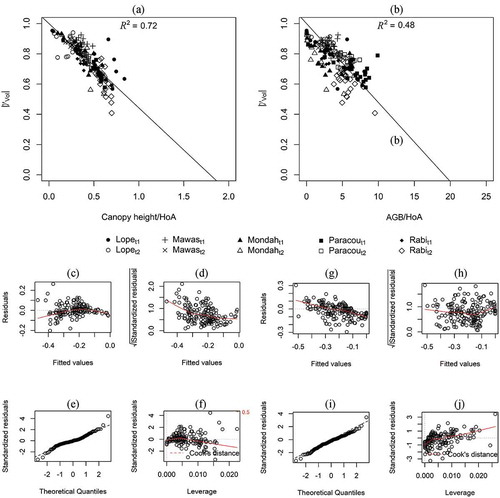
Table 3. Summary of the relationship between TanDEM-X coherence and canopy height as well as AGB (with a fixed intercept of 1)

Study area	Canopy height			AGB			$a_{h_{\mathrm{V}}}/a_{\mathrm{A}\mathrm{G}\mathrm{B}}$
	$a_{h_{\mathrm{V}}}$	$R_{h_{\mathrm{V}}}^2$	p-value	$a_{\mathrm{A}\mathrm{G}\mathrm{B}}$	$R_{\mathrm{A}\mathrm{G}\mathrm{B}}^2$	p-value
$\mathrm{L}\mathrm{o}\mathrm{p}{\mathrm{e}{ }^{\mathrm{\prime }}}_{t1}$	0.444	0.63	≤ 0.001	0.048	0.59	≤ 0.001	9.311
$\mathrm{L}\mathrm{o}\mathrm{p}{\mathrm{e}{ }^{\mathrm{\prime }}}_{t2}$	0.460	0.64	≤ 0.001	0.049	0.63	≤ 0.001	9.353
$\mathrm{M}\mathrm{a}\mathrm{w}\mathrm{a}{\mathrm{s}}_{t1}$	0.330	0.29	≤ 0.001	0.039	0.30	≤ 0.001	8.393
$\mathrm{M}\mathrm{a}\mathrm{w}\mathrm{a}{\mathrm{s}}_{t2}$	0.531	0.35	≤ 0.001	0.056	0.31	≤ 0.001	9.459
$\mathrm{M}\mathrm{o}\mathrm{n}\mathrm{d}\mathrm{a}{\mathrm{h}}_{t1}$	0.545	0.73	≤ 0.001	0.063	0.40	≤ 0.001	8.625
$\mathrm{M}\mathrm{o}\mathrm{n}\mathrm{d}\mathrm{a}{\mathrm{h}}_{t2}$	0.637	0.68	≤ 0.001	0.073	0.40	≤ 0.001	8.783
$\mathrm{P}\mathrm{a}\mathrm{r}\mathrm{a}\mathrm{c}\mathrm{o}{\mathrm{u}}_{t1}$	0.595	0.76	≤ 0.001	0.044	0.45	≤ 0.001	13.471
$\mathrm{P}\mathrm{a}\mathrm{r}\mathrm{a}\mathrm{c}\mathrm{o}{\mathrm{u}}_{t2}$	0.546	0.64	≤ 0.001	0.042	0.59	≤ 0.001	12.922
$\mathrm{R}\mathrm{a}\mathrm{b}{\mathrm{i}}_{t1}$	0.624	0.50	≤ 0.001	0.067	0.22	≤ 0.001	9.370
$\mathrm{R}\mathrm{a}\mathrm{b}{\mathrm{i}}_{t2}$	0.594	0.56	≤ 0.001	0.063	0.25	≤ 0.001	9.371
$\mathrm{A}\mathrm{l}{\mathrm{l}}_{t1}$	0.554	0.67	≤ 0.001	0.052	0.47	≤ 0.001	10.576
$\mathrm{A}\mathrm{l}{\mathrm{l}}_{t2}$	0.565	0.67	≤ 0.001	0.052	0.35	≤ 0.001	10.905
$\mathrm{A}\mathrm{l}{\mathrm{l}}_{t1+t2}$	0.558	0.72	≤ 0.001	0.052	0.48	≤ 0.001	10.680

The pooled data of all acquisitions resulted in a linear relationship of volume coherence and canopy height with a coefficient of determination of 0.72 and a slope of 0.56 (Figure 1 & Table 3). The slopes of the individual areas ranged from 0.33 in Mawas to 0.64 in Mondah. The coefficient of determination was generally above 0.50, except for the Mawas area where the coefficients of determination were 0.29 and 0.35 (Table 3).

The lowest coefficients of determination in the regression of volume coherence and AGB were also observed in Mawas. In general, the R² in the AGB regression was lower compared to the canopy height. The coefficients of determination ranged from 0.30 to 0.63 for the AGB, where the pooled data achieved a coefficient of determination of 0.48. The slope of the pooled data was 0.052 for the linear relationship between volume coherence and AGB, where it ranged in the individual areas from 0.039 in Mawas to 0.073 in Mondah (Table 3).

However, the different acquisition dates of each individual area generally resulted in similar slopes of the relationship for both variables. The largest difference was observed in Mawas, where the slopes differed by 0.2 for the canopy height and 0.02 for the AGB. Similarly, the pooled data with the first acquisition dates resulted in a similar slope compared to the pooled data with the second acquisition dates as well as to the pooled data with both acquisition dates for the canopy height and the AGB (Table 3).

The similarity between different acquisition dates was also confirmed by the SSIM index, where the three components l, c, and s as well as their product were considered. In general, the comparisons of the means (l) and standard deviations (c) generally revealed a similarity above 0.9. Lowest values of 0.93 were found for $l$ in Mawas and for c in Mondah. The comparisons of correlations (s) revealed in general values of 0.79 and higher. The only exception was Paracou, where the value was 0.13. This also resulted in the lowest overall SSIM value of 0.12 in Paracou, whereas the other SSIM values were 0.72 in Mondah to 0.85 in Rabi (Table 4).

Table 4. Average SSIM values of the two coherences in each study area

Study area	SSIM	l	c	s
$\mathrm{L}\mathrm{o}\mathrm{p}\mathrm{e}{ }^{\mathrm{\prime }}$	0.75	0.98	0.96	0.79
$\mathrm{M}\mathrm{a}\mathrm{w}\mathrm{a}\mathrm{s}$	0.82	0.93	0.98	0.90
$\mathrm{M}\mathrm{o}\mathrm{n}\mathrm{d}\mathrm{a}\mathrm{h}$	0.72	0.98	0.93	0.79
$\mathrm{P}\mathrm{a}\mathrm{r}\mathrm{a}\mathrm{c}\mathrm{o}\mathrm{u}$	0.12	0.99	0.94	0.13
$\mathrm{R}\mathrm{a}\mathrm{b}\mathrm{i}$	0.85	0.99	0.98	0.88

4.2. Estimation of canopy height and aboveground biomass

In the following, the model inversion for estimating canopy height is presented based on the pooled first date acquisitions in order to avoid auto-correlation due to dependent samples when combining first and second acquisition. The R² of the validated samples was 0.71 and the RMSE was 6.4 m (15.7%). Most errors and deviations from the 1:1 line were observed at higher canopy heights, which were in the order of the height of ambiguities of the used acquisitions (Figure 2). Furthermore, boxplots of canopy height residuals in each area indicated that this general model resulted in no substantial systematic over- or underestimation. Only the median in Lopé and Mawas indicated an underestimation of about 5 m. The medians of the residuals were about 0 m in the other areas, where the residuals were normally distributed (Figure 2).

Figure 2. Validation of the linear relationship between TanDEM-X volume coherence and canopy height with the pooled data from the first acquisitions (a) and the residuals in the individual areas (b)

Similarly to the canopy height, the model for estimating AGB was trained and validated with all acquisitions from the first date only. The R² of the validated samples was 0.59, where the RMSE was 88.2 t ha⁻¹. Consequently, the accuracy of the AGB estimation was generally lower compared to the canopy height. Again, the over- or underestimations were limited. However, a small overestimation was observed in Mondah and Rabi (Figure 3).

Figure 3. Validation of the linear relationship between TanDEM-X volume coherence and AGB with the pooled data from the first acquisitions (a) and the residuals in the individual areas (b)

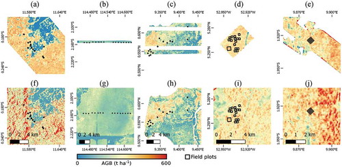
The spatial representation of the AGB estimation with ALS canopy height and TanDEM-X volume coherence confirmed the similarity between both estimations. In general, the spatial patterns were similar between ALS and TanDEM-X-based estimations (Figure 4). The lowest level of AGB was observed in Mawas, whereas the other areas had a generally higher AGB level. Lopé and Mondah showed a high dynamic range in AGB, where the AGB ranged from 0 t ha⁻¹ to about 600 t ha⁻¹. The largest visual discrepancies between the ALS and TanDEM-X-based estimation were observed in Lopé, where the TanDEM-X-based estimation indicated overestimations of the AGB (Figure 4). However, these were outside the plot locations and were therefore not part of the training and validation.

Figure 4. Spatial representation of the AGB estimated with ALS canopy height (a to e) and TanDEM-X volume coherence (f to j) in Lopé (a and f), Mawas (b and g), Mondah (c and h), Paracou (d and i) and Rabi (e and j)

The individual estimations had a generally similar R² compared to the estimation from the pooled data. The individual R² was higher in Mondah and Mawas compared to the R² from the pooled data in the canopy height estimation. The RMSE in m was lower in Mondah, Paracou, and Rabi compared to the pooled data. The R² in the AGB estimation was higher in Lopé and Paracou compared to the pooled data, whereas the RMSE in t ha⁻¹ was lower in Mawas, Paracou, and Rabi compared to the pooled data. However, the coefficients of determination and RMSE values did not differ substantially between the estimations with training and validation in the individual areas compared to the pooled data of all areas (Table 5).

Table 5. Summary of the validation for the estimations of canopy height and AGB based on TanDEM-X volume coherence trained with data from the individual areas and with the pooled data

Study area	Canopy height			AGB
	$R_{h_{\mathrm{V}}}^2$	RMSE (m)	RMSE (%)	$R_{\mathrm{A}\mathrm{G}\mathrm{B}}^2$	RMSE (t ha^−1)	RMSE (%)
Lopé	0.66	9.3	22.7	0.62	101.2	25.1
Mawas	0.73	7.6	43.7	0.55	63.5	16.8
Mondah	0.82	4.0	15.3	0.46	94.9	28.8
Paracou	0.40	4.0	32.6	0.71	75.1	17.8
Rabi	0.62	5.6	26.8	0.44	63.4	17.3
All	0.72	6.4	15.7	0.59	88.2	20.7

4.3. Estimation of canopy height and aboveground biomass with support from laser scanning data

The coefficient of determination of the regression between ALS canopy height and AGB was 0.68, where the slope coefficient $a_{\mathrm{A}\mathrm{L}\mathrm{S}}$ was 9.76 (Figure 5). Equation (9)(9) $a_{\mathrm{A}\mathrm{L}\mathrm{S}}=\frac{a_{h_{\mathrm{V}}}}{a_{\mathrm{A}\mathrm{G}\mathrm{B}}}$(9) suggests that the ratio of the slope coefficients of the linear relationship between volume coherence and canopy height as well as AGB equalled the slope coefficient of the regression between ALS canopy height and AGB. The ratio $a_{h_{\mathrm{V}}}/a_{\mathrm{A}\mathrm{G}\mathrm{B}}$ ranged from 8.4 to 13.5 for the different study areas. The smallest values were found in Mawas and Mondah, whereas the highest values were found in Paracou. The pooled data resulted in values of 10.6, 10.9, and 10.7 for this ratio (Table 3).

Figure 5. Linear relationship between ALS canopy height and AGB without intercept

The slope coefficient of the regression between ALS canopy height and AGB was used together with the slope of the canopy height and volume coherence regression to retrieve the slope of AGB and volume coherence regression ($a_{\mathrm{A}\mathrm{G}\mathrm{B}}=\frac{a_{h_{\mathrm{V}}}}{a_{\mathrm{A}\mathrm{L}\mathrm{S}}}$, where $a_{h_{\mathrm{V}}}$ was 0.554 and $a_{\mathrm{A}\mathrm{L}\mathrm{S}}$ was 9.76). This resulted in a $a_{\mathrm{A}\mathrm{G}\mathrm{B}}$ of 0.056. Similarly, the slope coefficient of the AGB and volume coherence regression was used together with $a_{\mathrm{A}\mathrm{L}\mathrm{S}}$ to estimate the slope coefficient of the canopy height and volume coherence regression ($a_{h_{\mathrm{V}}}=a_{\mathrm{A}\mathrm{G}\mathrm{B}}\times a_{\mathrm{A}\mathrm{L}\mathrm{S}}$). Consequently, in this estimation $a_{h_{\mathrm{V}}}$ was 0.547. Note that again only the first dates were used with 50% of the samples as training and 50% as validation in order to avoid dependent estimations. This slope coefficient was further used to estimate canopy height with volume coherence.

The estimations supported by the ALS canopy height resulted in R² values of 0.71 in the canopy height and 0.59 in the AGB estimation. The RMSEs were 6.7 m (16.4%) and 85.2 t ha⁻¹ (20.0%), where again no systematic over- or underestimation was observed (Figure 6). In general, the error distribution was similar compared to the estimations without support from the ALS canopy height (Figures 2, 3 and 6).

Figure 6. Validation of the linear relationship between TanDEM-X volume coherence and canopy height (a) as well as AGB (b) with the pooled data from the first acquisitions and slope coefficient estimated with the support of ALS data

5. Discussion

This study confirms that the volume coherence at X-band is related to forest structure attributes such as canopy height and AGB (Kugler et al. 2014; Treuhaft et al. 2015; Schlund et al. 2015; Olesk et al. 2016; Chen, Cloude, and Goodenough 2016; Schlund et al. 2019). Empirical functions were suggested to account for ambiguity effects in the linear and sinc relationship between TanDEM-X coherence and canopy height (Olesk et al. 2016; Chen, Cloude, and Goodenough 2016). Consequently, empirical functions were used to estimate canopy height in this study, which support the linear model for canopy height estimation. However, little is known about what determines the slope of the relationship. The selection of heights of ambiguity for this study was based on the fact that these heights of ambiguity are generally used for the global digital elevation model acquisition of TanDEM-X over forest areas. The relationship found might be applicable for a large range of forests acquired with similar height of ambiguities, even though the knowledge of what determines the slope of the relationship is limited. This was confirmed by the fact that the pooled data of all available study areas resulted in a similar slope and accuracy compared to the individual areas. Higher accuracies in the canopy height estimation in terms of R² and RMSE compared to this study could be achieved by using dual-polarized or full-polarized TanDEM-X data (Kugler et al. 2014; Khati, Singh, and Ferro-Famil 2017; Khati, Singh, and Kumar 2018). However, these datasets are not available on a global scale and are therefore limited in their applicability.

The AGB is a function of different tree attributes, which are reflected in allometric models, where the tree height is highly relevant (Chave et al. 2005, 2014; Jucker et al. 2017). The canopy height on plot, or stand level, was considered to have a high potential for estimating AGB (Neeff et al. 2005; Solberg et al. 2010; Schlund et al. 2016; Solberg et al. 2017; Schlund, Erasmi, and Scipal 2020; Knapp et al. 2020). Consequently, the volume coherence of TanDEM-X can be directly related to the AGB assuming that it can be used to estimate the canopy height. This direct relationship achieved an R² of 0.59 and an RMSE of 88.2 t ha⁻¹ (20.7%). Again, a linear relationship was considered appropriate between volume coherence and AGB. In general, the coefficients of determination as well as the relative RMSE indicated lower accuracy in the AGB estimation compared to the canopy height estimation with X-band coherence. This could be based on the fact that the interferometric coherence is related to the volume height (i.e. canopy height), which is further related to AGB. Consequently, errors and inaccuracies propagate in the AGB estimation. Despite potential inaccuracies in absolute AGB estimation, the estimated AGB indicates its spatial distribution and also different forest structure types, conditions of forests and forest degradation. This indication can support sampling schemes for forest stratification purposes (Schlund et al. 2015).

The results were found purely empirically, where a further understanding of the linear coefficients is necessary. Physical models are of relevance for improving the understanding of the empirically found relationships. Nevertheless, simplifications of the semi-empirical RVoG model support the findings of this study (Olesk et al. 2016; Schlund et al. 2019). The applicability of the relationships found should be studied further, as different regression coefficients could be also caused by topographical effects. This results in different estimations as can be seen in Lopé outside the forest plots, where the forest plots were generally acquired in flat terrain.

It is important to note that the calibration and validation in this study were based on forest plots in tropical forests. It was found that this could result in an erroneous overall AGB estimation and conclusions from outside of forests have limited validity (Schlund, Scipal, and Davidson 2017). Consequently, a forest classification is necessary to mask out non-forest areas, which could be created from TanDEM-X data or other data sources (Schlund et al. 2014; Baron and Erasmi 2017; Martone et al. 2018).

The similarity of $a_{\mathrm{A}\mathrm{L}\mathrm{S}}$ and $\frac{a_{h_{\mathrm{V}}}}{a_{\mathrm{A}\mathrm{G}\mathrm{B}}}$ confirms that ALS and TanDEM-X data provide complementary information. This is relevant since the globally consistent TanDEM-X data could complement the normally spatially limited ALS data. The canopy height models were information aggregated to plot level and thus were assumed to be determined by the canopy density and height, where the product of both was assumed proportional to the AGB (Treuhaft and Siqueira 2004; Solberg et al. 2013; Asner and Mascaro 2014). Therefore, previous studies revealed an insignificant exponent or an exponent close to one in the power-law form in the relationship of canopy height on plot level and AGB (e.g. Solberg et al. (2013); Asner and Mascaro (2014); Schlund and Davidson (2018)). Furthermore, the linear model of canopy height and AGB was considered easy to interpret enabling the comparison with the linear relationships of coherence and canopy height as well as AGB. Therefore, the linear relationship between canopy height and AGB was similar to other studies assumed appropriate (Neeff et al. 2005; Solberg et al. 2010; Schlund et al. 2016; Solberg et al. 2017; Schlund, Erasmi, and Scipal 2020). The canopy height and AGB estimation can be calibrated and validated in a limited number of areas with ALS coverage, which are further applied to TanDEM-X data to provide canopy height and AGB information on a larger spatial scale. A combined estimation of canopy height with spaceborne LiDAR data (e.g. GEDI) and TanDEM-X was suggested in previous studies (Qi and Dubayah 2016; Qi et al. 2019). This could potentially bridge the gap between in situ measurements and spaceborne data (Réjou-Méchain et al. 2019). Furthermore, the results of this study suggest that the estimations were consistent for the different acquisitions on plot level and on spatial level indicated by the SSIM. The TanDEM-X data from the same orbit direction were generally highly similar with SSIM values of higher than 0.7. The similarity in terms of correlation decreased with data from different orbit directions resulting in lowest SSIM, as was observed in Paracou. Consequently, the consistency between acquisitions was highest for the same orbit directions and to achieve the highest accuracies the general models should be calibrated and validated individually for the orbit directions. However, the similarity of local contrasts in magnitude (i.e. mean l and variance c) was also highly similar in Paracou, which means that the canopy height and AGB estimation was highly similar in their spatial average and variance.

It was assumed that in the analysis no change occurred between the different TanDEM-X acquisitions as well as between the in situ and ALS data acquisitions. This is one potential source of error in this analysis (Réjou-Méchain et al. 2019). However, the observed forests were generally mature and it can be assumed that forest growth was negligible in the time frames of the acquisitions. Furthermore, the forest plots were located in stable areas with low frequencies of change, where some of the forest plots were even located in protected areas. For instance, the Mawas area with the largest temporal discrepancy between the acquisition dates is a conservation area. This area was assumed to be undisturbed with stable AGB and even increase of AGB in the eastern part of the Mawas area (Schlund et al. 2015; Wedeux et al. 2020), where only few plots were sampled. However, the reported growth rate by Wedeux et al. (2020) was lower than the error of the AGB estimation. The lowest coefficient of determination in Mawas compared to the other areas could be also based on the fact that the area had the lowest range and variability of canopy height and AGB. Consequently, changes based on deforestation, forest degradation, or growth were neglected in this study.

6. Conclusion

The estimation of forest structure attributes is important for the assessment of the global carbon cycle. The study revealed that TanDEM-X has the potential to provide information about canopy height and AGB with accuracies of 16% and 21% across five different study areas in the tropics. The extensive empirical analysis confirms the generality of a linear relationship between X-band volume coherence and canopy height as well as AGB. The results suggest a relationship between LiDAR and X-band coherence, which could help to bridge the gap from sampled ALS or spaceborne LiDAR acquisitions to consistent wall-to-wall coverage with the globally available TanDEM-X data. The volume coherence of TanDEM-X could at least provide the spatial distribution of canopy height and AGB indicating the status of the forest in general, despite potential errors in the absolute canopy height and AGB derivatives. Such a stratification would be useful as a prerequisite for efficient forest inventories, which are of relevance in national carbon accounting and REDD+ projects (GOFC-GOLD 2012; Schlund et al. 2015).

Acknowledgements

TanDEM-X data used within this work were provided by DLR. The authors would like to thank B. Herault and A. Dourdain from CIRAD for providing the LiDAR data of Paracou. LVIS data sets were provided by the Land, Vegetation, and Ice Sensor (LVIS) team in Code 61A at NASA Goddard Space Flight Center, with support from the University of Maryland, College Park, MD, USA. The LVIS data sets are accessible via http://lvis.gsfc.nasa.gov. We would like to thank the field teams and plot owners for conducting the in situ measurements and also Klaus Scipal for his support in the data acquisition. The plot data of Gabon and French Guiana can be accessed via forest-observation-system.net. BOS is acknowledged for the support during the Mawas field campaign.

Disclosure statement

No potential conflict of interest was reported by the authors.

Correction Statement

This article has been republished with minor changes. These changes do not impact the academic content of the article.

Additional information

Funding

This work was supported in part by the Federal Ministry for Economic Affairs and Energy (BMWi) as part of the Project IKEBANA under Grant no. 50EE1808B and the German Academic Exchange Service.

References

- Asner, G. P. 2009. “Tropical Forest Carbon Assessment: Integrating Satellite and Airborne Mapping Approaches.” Environmental Research Letters 4 (3): 1–11. doi:10.1088/1748-9326/4/3/034009.
- Asner, G. P., and J. Mascaro. 2014. “Mapping Tropical Forest Carbon: Calibrating Plot Estimates to a Simple LiDAR Metric.” Remote Sensing of Environment 140: 614–624. doi:10.1016/j.rse.2013.09.023.
- Baccini, A., S. J. Goetz, W. S. Walker, N. T. Laporte, M. Sun, D. Sulla-Menashe, J. Hackler, et al. 2012. “Estimated Carbon Dioxide Emissions from Tropical Deforestation Improved by Carbon-density Maps.” Nature Climate Change 2 (3): 182–185. doi:10.1038/nclimate1354.
- Baron, D., and S. Erasmi. 2017. “High Resolution Forest Maps from Interferometric TanDEM-X and Multitemporal Sentinel-1 SAR Data.” PFG - Journal of Photogrammetry, Remote Sensing and Geoinformation Science 85 (6): 389–405. doi:10.1007/s41064-017-0040-1.
- Blair, J. B., M. A. Hofton, and D. L. Rabine. 2018. Processing of NASA LVIS Elevation and Canopy (LGE, LCE and LGW) Data Products. NASA Goddard Space Flight Center. Maryland.
- Blair, J. B., D. L. Rabine, and M. A. Hofton. 1999. “The Laser Vegetation Imaging Sensor (LVIS): A Medium-altitude, Digitization-only, Airborne Laser Altimeter for Mapping Vegetation and Topography.” ISPRS Journal of Photogrammetry and Remote Sensing 54 (2–3): 115–122. doi:10.1016/S0924-2716(99)00002-7.
- Castro, K. L., G. A. Sanchez-Azofeifa, and B. Rivard. 2003. “Monitoring Secondary Tropical Forests Using Space-borne Data: Implications for Central America.” International Journal of Remote Sensing 24 (9): 1853–1894. doi:10.1080/01431160210154056.
- Chave, J., M. Rejou-Mechain, A. Burquez, E. Chidumayo, M. S. Colgan, W. B. C. Delitti, A. Duque, et al. 2014. “Improved Allometric Models to Estimate the Aboveground Biomass of Tropical Trees.” Global Change Biology 20 (10): 3177–3190. doi:10.1111/gcb.12629.
- Chave, J., C. Andalo, S. Brown, M. A. Cairns, J. Q. Chambers, D. Eamus, H. Folster, et al. 2005. “Tree Allometry and Improved Estimation of Carbon Stocks and Balance in Tropical Forests.” Oecologia 145 (1): 87–99. doi:10.1007/s00442-005-0100-x.
- Chave, J., D. Coomes, S. Jansen, S. L. Lewis, N. G. Swenson, and A. E. Zanne. 2009. “Towards a Worldwide Wood Economics Spectrum.” Ecology Letters 12 (4): 351–366. doi:10.1111/j.1461-0248.2009.01285.x.
- Chen, H., S. R. Cloude, and D. G. Goodenough. 2016. “Forest Canopy Height Estimation Using TanDEM-X Coherence Data.” IEEE Journal of Selected Topics in Applied Earth Observations and Remote Sensing 9 (7): 3177–3188. doi:10.1109/JSTARS.2016.2582722.
- Chen, H., S. R. Cloude, D. G. Goodenough, D. A. Hill, and A. Nesdoly. 2018. “Radar Forest Height Estimation in Mountainous Terrain Using Tandem-X Coherence Data.” IEEE Journal of Selected Topics in Applied Earth Observations and Remote Sensing 11 (10): 3443–3452. doi:10.1109/JSTARS.2018.2866059.
- Dubois-Fernandez, P., T. Le Toan, J. Chave, L. Blanc, S. Daniel, H. Oriot, A. Arnaubec, et al. 2011. TropiSAR 2009 - Technical Assistance for the Development of Airborne SAR and Geophysical Measurements during the TropiSAR 2009 Experiment. Vol. 2.1. ESA/CNES. Noordwijk.
- Dubois-Fernandez, P. C., T. Le Toan, S. Daniel, H. Oriot, J. Chave, L. Blanc, L. Villard, M. Davidson, and M. Petit. 2012. “The TropiSAR Airborne Campaign in French Guiana: Objectives, Description, and Observed Temporal Behavior of the Backscatter Signal.” IEEE Transactions on Geoscience and Remote Sensing 50 (8): 3228–3241. doi:10.1109/TGRS.2011.2180728.
- Duque, S., U. Balls, C. Rossi, T. Fritz, and W. Balzer. 2012. TanDEM-X. Ground Segment. CoSSC Generation and Interferometric Considerations. Issue: 1.0. Oberpfaffenhofen: Deutsches Zentrum fuer Luft- und Raumfahrt (DLR).
- Faraway, J. J. 2006. Extending the Linear Model with R. Generalized Linear, Mixed Effects and Nonparametric Regression Models. Boca Raton: Chapman & Hall/CRC.
- Fritz, T. 2012. TanDEM-X. Ground Segment. TanDEM-X Experimental Product Description. Issue: 1.2. Oberpfaffenhofen: Deutsches Zentrum fuer Luft- und Raumfahrt (DLR).
- GCOS. 2015. Status of the Global Observing System for Climate. WMO. GCOS-195. Geneva.
- Gibbs, H. K., S. Brown, J. O. Niles, and J. A. Foley. 2007. “Monitoring and Estimating Tropical Forest Carbon Stocks: Making REDD a Reality.” Environmental Research Letters 2: 1–13. doi:10.1088/1748-9326/2/4/045023.
- GOFC-GOLD. 2012. A sourcebook of methods and procedures for monitoring and reporting an-thropogenic greenhouse gas emissions and removals associated with deforestation, gains and losses of carbon stocks in forests remaining forests, and forestation. GOFC-GOLD Report version COP18-1. Wageningen: Wageningen University.
- Hu, T., Y. Su, B. Xue, J. Liu, X. Zhao, J. Fang, and Q. Guo. 2016. “Mapping Global Forest Aboveground Biomass with Spaceborne LiDAR, Optical Imagery, and Forest Inventory Data.” Remote Sensing 8 (7): 565–591. doi:10.3390/rs8070565.
- Imhoff, M. L. 1995. “Radar Backscatter and Biomass Saturation: Ramifications for Global Biomass Inventory.” IEEE Transactions on Geoscience and Remote Sensing 33 (2): 511–518. doi:10.1109/TGRS.1995.8746034.
- Joetzjer, E., M. Pillet, P. Ciais, N. Barbier, J. Chave, M. Schlund, F. Maignan, et al. 2017. “Assimilating Satellite-based Canopy Height within an Ecosystem Model to Estimate Aboveground Forest Biomass.” Geophysical Research Letters 44 (13): 6823–6832. https://agupubs.onlinelibrary.wiley.com/doi/abs/10.1002/2017GL074150
- Jones, E. L., L. Rendell, E. Pirotta, and J. A. Long. 2016. “Novel Application of a Quantitative Spatial Comparison Tool to Species Distribution Data.” Ecological Indicators 70: 67–76. doi:10.1016/j.ecolind.2016.05.051.
- Jucker, T., J. Caspersen, J. Chave, C. Antin, N. Barbier, F. Bongers, M. Dalponte, et al. 2017. “Allometric Equations for Integrating Remote Sensing Imagery into Forest Monitoring Programmes.” Global Change Biology 23 (1): 177–190. https://onlinelibrary.wiley.com/doi/abs/10.1111/gcb.13388
- Khati, U., G. Singh, and S. Kumar. 2018. “Potential of Space-Borne PolInSAR for Forest Canopy Height Estimation over India - A Case Study Using Fully Polarimetric L-, C-, and X-Band SAR Data.” IEEE Journal of Selected Topics in Applied Earth Observations and Remote Sensing 11 (7): 2406–2416. doi:10.1109/JSTARS.2018.2835388.
- Khati, U., G. Singh, and L. Ferro-Famil. 2017. “Analysis of Seasonal Effects on Forest Parameter Estimation of Indian Deciduous Forest Using TerraSAR-X PolInSAR Acquisitions.” Remote Sensing of Environment 199: 265–276. doi:10.1016/j.rse.2017.07.019.
- Knapp, N., R. Fischer, V. Cazcarra-Bes, and A. Huth. 2020. “Structure Metrics to Generalize Biomass Estimation from Lidar across Forest Types from Different Continents.” Remote Sensing of Environment 237: 111597. doi:10.1016/j.rse.2019.111597.
- Krieger, G., A. Moreira, H. Fiedler, I. Hajnsek, M. Werner, M. Younis, and M. Zink. 2007. “TanDEM-X: A Satellite Formation for High-Resolution SAR Interferometry.” IEEE Transactions on Geoscience and Remote Sensing 45 (11): 3317–3341. doi:10.1109/TGRS.2007.900693.
- Kugler, F., D. Schulze, I. Hajnsek, H. Pretzsch, and K. P. Papathanassiou. 2014. “TanDEM-X Pol-InSAR Performance for Forest Height Estimation.” IEEE Transactions on Geoscience and Remote Sensing 52 (10): 6404–6422. doi:10.1109/TGRS.2013.2296533.
- Kutner, M. H., C. J. Nachtsheim, J. Neter, M. H. Li, W. Kutner, C. J. Nachtsheim, J. Neter, and W. Li. 2005. Applied Linear Statistical Models. 5th ed. New York: McGraw-Hill/Irwin.
- Labriere, N., S. Tao, J. Chave, K. Scipal, T. L. Toan, K. Abernethy, A. Alonso, et al. 2018. “In Situ Reference Datasets from the TropiSAR and AfriSAR Campaigns in Support of Upcoming Spaceborne Biomass Missions.” IEEE Journal of Selected Topics in Applied Earth Observations and Remote Sensing 11 (10): 3617–3627. doi:10.1109/JSTARS.2018.2851606.
- Le Toan, T., A. Beaudoin, J. Riom, and D. Guyon. 1992. “Relating Forest Biomass to SAR Data.” IEEE Transactions on Geoscience and Remote Sensing 30 (2): 403–411. doi:10.1109/36.134089.
- Lefsky, M. A., D. J. Harding, M. Keller, W. B. Cohen, C. C. Carabajal, F. Del Bom Espirito-Santo, M. O. Hunter, and R. de Oliveira. 2005. “Estimates of Forest Canopy Height and Aboveground Biomass Using ICESat.” Geophysical Research Letters 32 (22): 1–4. doi:10.1029/2005GL023971.
- Liu, Y. Y., I. J. M. Albert, R. A. van Dijk, M. de Jeu, J. G. Canadell, M. F. McCabe, J. P. Evans, and G. Wang. 2015. “Recent Reversal in Loss of Global Terrestrial Biomass.” Nature Climate Change 5: 470–474. doi:10.1038/nclimate2581.
- Martone, M., B. Braeutigam, P. Rizzoli, C. Gonzalez, M. Bachmann, and G. Krieger. 2012. “Coherence Evaluation of TanDEM-X Interferometric Data.” ISPRS Journal of Photogrammetry and Remote Sensing 73: 21–29. doi:10.1016/j.isprsjprs.2012.06.006.
- Martone, M., P. Rizzoli, C. Wecklich, C. González, J.-L. Bueso-Bello, P. Valdo, D. Schulze, M. Zink, G. Krieger, and A. Moreira. 2018. “The Global Forest/non-forest Map from TanDEM-X Interferometric SAR Data.” Remote Sensing of Environment 205: 352–373. doi:10.1016/j.rse.2017.12.002.
- Molto, Q., B. Hérault, -J.-J. Boreux, M. Daullet, A. Rousteau, and V. Rossi. 2014. “Predicting Tree Heights for Biomass Estimates in Tropical Forests - a Test from French Guiana.” Biogeosciences 11 (12): 3121–3130. doi:10.5194/bg-11-3121-2014.
- Neeff, T., L. V. Dutra, J. R. Dos Santos, C. D. C. Freitas, and L. S. Araujo. 2005. “Tropical Forest Measurement by Interferometric Height Modeling and P-Band Radar Backscatter.” Forest Science 51 (6): 585–594. http://www.ingentaconnect.com/content/saf/fs/2005/00000051/00000006/art00009.
- Olesk, A., J. Praks, O. Antropov, K. Zalite, T. Arumae, and K. Voormansik. 2016. “Interferometric SAR Coherence Models for Characterization of Hemiboreal Forests Using TanDEM-X Data.” Remote Sensing 8 (700): 1–23. doi:10.3390/rs8090700.
- Pan, Y., R. A. Birdsey, J. Fang, R. Houghton, P. E. Kauppi, W. A. Kurz, O. L. Phillips, et al. 2011. “A Large and Persistent Carbon Sink in the World’s Forests.” Science 333 (6045): 988–993. http://science.sciencemag.org/content/333/6045/988
- Pitz, W., and D. Miller. 2010. “The TerraSAR-X Satellite.” IEEE Transactions on Geoscience and Remote Sensing 48 (2): 615–622. doi:10.1109/TGRS.2009.2037432.
- Qi, W., and R. O. Dubayah. 2016. “Combining Tandem-X InSAR and Simulated GEDI Lidar Observations for Forest Structure Mapping.” Remote Sensing of Environment 187: 253–266. doi:10.1016/j.rse.2016.10.018.
- Qi, W., S.-K. Lee, S. Hancock, S. Luthcke, H. Tang, J. Armston, and R. Dubayah. 2019. “Improved Forest Height Estimation by Fusion of Simulated GEDI Lidar Data and TanDEM-X InSAR Data.” Remote Sensing of Environment 221: 621–634. doi:10.1016/j.rse.2018.11.035.
- Réjou-Méchain, M., N. Barbier, P. Couteron, P. Ploton, G. Vincent, M. Herold, S. Mermoz, et al. 2019. “Upscaling Forest Biomass from Field to Satellite Measurements: Sources of Errors and Ways to Reduce Them”. Surveys in Geophysics 40: 881–911. doi:10.1007/s10712-019-09532-0.
- Saatchi, S. S., N. L. Harris, S. Brown, M. Lefsky, E. T. A. Mitchard, W. Salas, B. R. Zutta, et al. 2011. “Benchmark Map of Forest Carbon Stocks in Tropical Regions across Three Continents.” Proceedings of the National Academy of Science of the United States of America (PNAS) 108 (24): 9899–9904. doi:10.1073/pnas.1019576108.
- Schepaschenko, D., J. Chave, O. L. Phillips, S. L. Lewis, S. J. Davies, M. Réjou-Méchain, P. Sist, et al. 2019a. “The Forest Observation System, Building a Global Reference Dataset for Remote Sensing of Forest Biomass.” Scientific Data 6 (198): 1–11. doi:10.1038/s41597-019-0196-1.
- Schepaschenko, D., J. Chave, O. L. Phillips, S. L. Lewis, S. J. Davies, M. Réjou-Méchain, P. Sist, et al. 2019b. “A Global Reference Dataset for Remote Sensing of Forest Biomass. The Forest Observation System Approach.” Technical Report. Forest Observation System.
- Schlund, M., and M. W. J. Davidson. 2018. “Aboveground Forest Biomass Estimation Combining L- and P-Band SAR Acquisitions.” Remote Sensing 10 (7): 1–23. doi:10.3390/rs10071151.
- Schlund, M., S. Erasmi, and K. Scipal. 2020. “Comparison of Aboveground Biomass Estimation from InSAR and LiDAR Canopy Height Models in Tropical Forests.” IEEE Geoscience and Remote Sensing Letters 17 (3): 367–371. doi:10.1109/LGRS.2019.2925901.
- Schlund, M., F. V. Poncet, S. Kuntz, H. D.-V. Boehm, D. Hoekman, and C. Schmullius. 2016. “TanDEM-X Elevation Model Data for Canopy Height and Aboveground Biomass Retrieval in a Tropical Peat Swamp Forest.” International Journal of Remote Sensing 37 (21): 5021–5044. doi:10.1080/01431161.2016.1226001.
- Schlund, M., P. Magdon, B. Eaton, C. Aumann, and S. Erasmi. 2019. “Canopy Height Estimation with TanDEM-X in Temperate and Boreal Forests.” International Journal of Applied Earth Observation and Geoinformation 82: 101904. doi:10.1016/j.jag.2019.101904.
- Schlund, M., K. Scipal, and M. W. J. Davidson. 2017. “Forest Classification and Impact of BIOMASS Resolution on Forest Area and Aboveground BIOMASS Estimation.” International Journal of Applied Earth Observation and Geoinformation 56: 65–76. doi:10.1016/j.jag.2016.12.001.
- Schlund, M., F. von Poncet, D. H. Hoekman, S. Kuntz, and C. Schmullius. 2014. “Importance of Bistatic SAR Features from TanDEM-X for Forest Mapping and Monitoring.” Remote Sensing of Environment 151: 16–26. doi:10.1016/j.rse.2013.08.024.
- Schlund, M., F. von Poncet, S. Kuntz, C. Schmullius, and D. H. Hoekman. 2015. “TanDEM-X Data for Aboveground Biomass Retrieval in a Tropical Peat Swamp Forest.” Remote Sensing of Environment 158: 255–266. doi:10.1016/j.rse.2014.11.016.
- Silva, C. A., S. Saatchi, M. Garcia, N. Labriere, C. Klauberg, A. Ferraz, V. Meyer, et al. 2018. “Comparison of Small- and Large-Footprint Lidar Characterization of Tropical Forest Aboveground Structure and Biomass: A Case Study from Central Gabon.” IEEE Journal of Selected Topics in Applied Earth Observations and Remote Sensing 11 (10): 3512–3526. doi:10.1109/JSTARS.2018.2816962.
- Solberg, S., D. J. Weydahl, and R. Astrup. 2015. “Temporal Stability of X-Band Single-Pass InSAR Heights in a Spruce Forest: Effects of Acquisition Properties and Season.” IEEE Transactions on Geoscience and Remote Sensing 53 (3): 1607–1614. doi:10.1109/TGRS.2014.2346473.
- Solberg, S., R. Astrup, J. Breidenbach, B. Nilsen, and D. Weydahl. 2013. “Monitoring Spruce Volume and Biomass with InSAR Data from TanDEM-X.” Remote Sensing of Environment 139: 60–67. doi:10.1016/j.rse.2013.07.036.
- Solberg, S., R. Astrup, T. Gobakken, E. Naesset, and D. J. Weydahl. 2010. “Estimating Spruce and Pine Biomass with Interferometric X-band SAR.” Remote Sensing of Environment 114 (10): 2353–2360. doi:10.1016/j.rse.2010.05.011.
- Solberg, S., E. H. Hansen, T. Gobakken, E. Naessset, and E. Zahabu. 2017. “Biomass and InSAR Height Relationship in a Dense Tropical Forest.” Remote Sensing of Environment 192: 166–175. doi:10.1016/j.rse.2017.02.010.
- Treuhaft, R., F. Goncalves, J. R. Dos Santos, M. Keller, M. Palace, S. N. Madsen, F. Sullivan, and P. M. L. A. Graca. 2015. “Tropical-Forest Biomass Estimation at X-Band from the Spaceborne TanDEM-X Interferometer.” IEEE Geoscience and Remote Sensing Letters 12 (2): 239–243. doi:10.1109/LGRS.2014.2334140.
- Treuhaft, R. N., and P. R. Siqueira. 2004. “The Calculated Performance of Forest Structure and Biomass Estimates from Interferometric Radar.” Waves in Random Media 14 (2): 345–358. doi:10.1088/0959-7174/14/2/013.
- Walters, G., E. N. Ndjabounda, D. Ikabanga, J. P. Biteau, O. Hymas, L. J. T. White, A.-M. Ndong Obiang, et al. 2016. “Peri-urban Conservation in the Mondah Forest of Libreville, Gabon: Red List Assessments of Endemic Plant Species, and Avoiding Protected Area Downsizing.” Oryx 50 (3): 419–430.
- Wang, Z., A. C. Bovik, H. R. Sheikh, and E. P. Simoncelli. 2004. “Image Quality Assessment: From Error Visibility to Structural Similarity.” IEEE Transactions on Image Processing 13 (4): 600–612. doi:10.1109/TIP.2003.819861.
- Wedeux, B., M. Dalponte, M. Schlund, S. Hagen, M. Cochrane, L. Graham, A. Usup, A. Thomas, and D. Coomes. 2020. “Dynamics of a Human-modified Tropical Peat Swamp Forest Revealed by Repeat Lidar Surveys.” Global Change Biology 26 (7): 3947–3964. doi:10.1111/gcb.15108.
- Yang, H., P. Ciais, M. Santoro, Y. Huang, W. Li, Y. Wang, A. Bastos, et al. 2020. “Comparison of Forest Above-ground Biomass from Dynamic Global Vegetation Models with Spatially Explicit Remotely Sensed Observation-based Estimates.” Global Change Biology 26 (7): 3997–4012. https://onlinelibrary.wiley.com/doi/abs/10.1111/gcb.15117