Heading variations resolve the heading-direction ambiguity in vertical-beam radar observations of insect migration

ABSTRACT

Vertical-beam entomological radars provide precise measurements of the body alignment of individual overflying insects but are unable to distinguish which of the two axial directions the insect is heading towards. Insects migrating at altitude typically show common alignment, although with a broad spread. We show here that when observations from multiple individual insects are available, and the insects have airspeeds of about 2 ms^–1 or greater, the spread in heading directions allows the heading ambiguity to be resolved (though at the sample rather than the individual level). A vector analysis of radar-measured track direction, track speed, and heading will provide consistent results for all the insects in a sample only when the heading direction is chosen correctly. With the heading then resolved, the analysis can continue to estimation of representative values for the airspeed of the insects in the sample and for the speed and direction of the wind they were flying in. This general approach can be implemented in two different ways, which we term the ‘cluster’ and ‘projection’ methods. When applied to an intense migration of large insects, probably moths, these methods produced highly consistent results from hour to hour and from one 150 m height interval to the next. Simulations show that the methods are not liable to directional bias and reveal when they are rendered ineffective by small sample sizes or low insect airspeeds; they also indicate that the cluster method handles small sample sizes better than the projection method, and its use is therefore recommended. A comparison with two previously proposed methods that use meteorological data to resolve the ambiguity shows that the new methods are more reliable. Use of this objective means of resolving the heading ambiguity will increase confidence in radar-based studies of the orientation behaviour of insect migrants and their responses to cues like sky illumination patterns, the Earth’s magnetic field, and wind.

1. Introduction

Very large numbers of insects take to the air, by day and by night, to undertake movements over hundreds of kilometres that constitute a form of migration, i.e. that lead to populations breeding in a region distant from that in which they had arisen (Johnson 1969; Chapman et al. 2015; Reynolds, Chapman, and Drake 2017). These movements enable populations to exploit host plants and prey as these arise at different latitudes and in different seasons, with significant economic and humanitarian impact when the migrants are crop pests (Drake and Gatehouse 1995; Chapman et al. 2012). Insect migrations also lead to transfers between regions of biomass, essential elements, pollen, and pathogens of plant, animal, and human diseases (Reynolds, Chapman, and Harrington 2006; Hu et al. 2016a; Huestis et al. 2019; Satterfield et al. 2020). In most cases, insect migratory flight is primarily windborne, and occurs at altitudes of a few hundred metres (Drake 1984; Reynolds, Chapman, and Drake 2017). Our knowledge of these migrations is derived mainly from sampling with balloon-, kite-, or aircraft-borne nets (e.g. Johnson 1969; Huestis et al. 2019) and, predominantly in the modern era, through observation with radar (Drake and Reynolds 2012).

An almost universal finding of radar studies of insect migration is that the migrants exhibit common orientation, i.e. insects flying at similar times and heights head in similar directions (Schaefer 1976; Riley and Reynolds 1986; Hu et al. 2016b). Potential advantages conferred by this behaviour, which occurs even at night in insects flying hundreds of metres above the surface, include greater distance covered or movement in a more favourable direction (e.g. Chapman et al. 2010). Both the mechanisms by which the heading is determined and maintained, and the way it benefits the migrant, are currently the subject of significant research effort (e.g. Reynolds et al. 2016; Dreyer et al. 2018; Wotton et al. 2019; Adden 2020). A major difficulty that radar-based studies have faced is that radars provide estimates of insect body alignments rather than headings; i.e. they provide an angle, often quite precise, in the range 0° to 180°, but are not able to determine whether this is the direction the insect is heading towards or the direction it is heading away from. This is the case both for the vertical-beam systems developed specifically for insect observation, e.g. of the type known variously as Vertical-Looking Radars (VLR) and Insect Monitoring Radars (IMR) (Chapman, Reynolds, and Smith 2003; Drake et al. 2020), and radars in which the beam is scanned (e.g. Schaefer 1976). With scanning radars, differences in the echo signals from the two possible directions can sometimes be discerned, but these are not easily interpreted (Drake 1983; Melnikov, Istok, and Westbrook 2015). In this article, we present two variants of a novel approach to resolving this ‘heading-direction ambiguity’ in the observation datasets provided by VLRs and IMRs, in which measurement data are obtained for individual insects. We show also that the new procedures allow estimation of both a representative airspeed for the migrant population and the direction and speed of the wind that the insects are flying in.

An insect’s movement over the ground arises from the vector sum of its own airspeed and heading and that of the wind at the height it is flying. If the movement and wind vectors are known, the flight speed and direction are easily estimated by vector subtraction. The alignment ambiguity could then be resolved by adopting the direction closest to the estimated flight direction. When winds are strong, the contribution of the insect’s airspeed may be relatively small and movement and wind measurements that are both precise and accurate will be needed to determine the flight vector. We have previously explored this approach with movement data from an IMR operating in inland eastern Australia and winds obtained from reanalysed operational meteorological observations via a dynamic downscaling process, with mixed results (Hao, Drake, and Taylor 2019; and see below). By drawing only on IMR data, i.e. data from a single observing system, the new methods eliminate a potential source of systematic error. They exploit the variation in alignment directions within a sample of measurements to determine, again by vector subtraction, which of the two possible heading directions provides a consistent estimate of the wind. In order to verify the underlying approach and its specific implementations, the two methods have been applied to a 15-night observation dataset and also examined through simulation. The latter is useful particularly for assessing the sensitivity of the methods and the likelihood of biases arising through their use.

2. Materials and methods

While the two methods exploit the same information content in the data, they do so in rather different ways. We document both here to allow the advantages and drawbacks of each to be recognized, and to enable a recommendation to be made on which one to adopt for general use.

2.1. Cluster method

The basis of the first method, which is essentially an extension of an analysis developed for photographic recordings of locust flights within swarms (Rainey 1989, his Figure 104), is illustrated in the vector diagrams of Figure 1(a–c). An insect flying through the air with airspeed and heading direction v_F (the ‘flight vector’) is carried along by the wind v_W, producing a movement over the ground (or ‘track’) v_T that is the vector sum of these two quantities (Figure 1(a)). (Vertical motion is assumed negligible and not represented.) The dashed lines in Figure 1(a) represent a second insect moving in the same airflow and flying at the same airspeed, but with a different heading. The measurements produced by the radar comprise both components of v_T (speed and direction) and the alignment direction φ_A, represented in Figure 1(b) by a double-headed arrow (the length of which has no significance); the wind vector v_W and the insects’ airspeeds are unknown. [An insect’s transit of a VLR’s or IMR’s narrow (about 1°) vertical beam lasts only a few seconds and is well represented by motion with unchanging speed and direction (Harman and Drake 2004; Drake and Reynolds 2012, pp. 144–159).] Measurements for a single insect do not allow v_W to be determined: the vector could end anywhere on the dotted line drawn along the alignment axis. If an airspeed is assumed, the number of possible endpoints is reduced to two (blue dots, drawn for an assumed airspeed slightly lower than the actual one), but which of these is the correct one cannot be resolved from the measured values v_T,m and φ_A,m alone. However, it is readily seen (Figure 1(b)) that when measurements from a second insect that is experiencing the same wind, but has a different alignment, are available, the alignment axes will intersect and not only is the heading direction ambiguity resolved but values for the airspeed and the wind can be estimated.

Figure 1. Vector triangles illustrating cluster method for resolving the heading direction ambiguity and estimating airspeed and wind. In this example, the wind speed is twice the insect’s airspeed. (a) Vector triangles for two insects with different headings. (b) Resolution of ambiguity from available measurements for two insects with no random variation. (c) Resolution for multiple insects with random variation; for clarity, only the endpoints (green dots) of the track vectors are shown. Diagonal crosses indicate the centroids of the two sets of blue points. Key: N, north; O, origin (where speeds are zero); A, alignment of insect; F, flight of insect through the air; T, track of insect; W, wind; m, a measured value, e, an estimated value

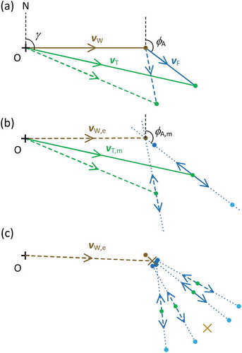
A more realistic scenario is illustrated in Figure 1(c), in which v_T,m and φ_A,m values for additional insects are available but these are now subject to random variation, so that the alignment axes will not all meet at one point. A practicable procedure for dealing with this is to assume a common airspeed for all the insects in the sample, and then determine the two sets of endpoints (blue dots). It is evident that they form two clusters, one compact and the other spread out and in the form of an arc. Selection of the smaller cluster resolves the heading direction ambiguity, and its centroid provides estimates for the speed v_W and direction φ_W of the wind. This procedure can be repeated for a range of plausible airspeeds, with whichever produces the most compact cluster being adopted as the estimate of an airspeed representative of the sample; the centroid wind values obtained with this airspeed provide the final estimate of the wind experienced by the insects in the sample.

A more formal statement of the procedure illustrated in Figure 1(c) is now presented. First, the track vectors v_T are calculated, in Cartesian coordinates, for each insect i as

(1) $v_{\mathrm{T},x,i}=v_{\mathrm{T},m,i}sin{\gamma }_{m,i},v_{\mathrm{T},y,i}=v_{\mathrm{T},m,i}cos{\gamma }_{m,i}$(1)

where (v_T,m,i, γ_m,i) are the insect’s measured movement speed and direction (the latter defined as clockwise from N), the x coordinate represents movement to E, and the y coordinate movement to N. These are the coordinates of the green dots. For each assumed airspeed value a_j, components of the flight vectors v_F,j,i are then calculated for each insect i, using the measured alignment φ_A,m,i,

(2) $v_{\mathrm{F},x,j,i}=a_{j}sin{\phi }_{\mathrm{A},m,i},v_{\mathrm{F},y,j,i}=a_{j}cos{\phi }_{\mathrm{A},m,i}$(2)

The wind can be estimated by subtracting the flight vector from the track vector (Figure 1(a)), but as the airspeed is not yet determined and there are two possible flight vectors for each insect, we will follow Hao, Drake, and Taylor (2019) and refer to these estimates as ‘putative winds’ v_P. The first of each pair is calculated by subtracting v_F from v_T and the second by adding these two vectors.

$v_{\mathrm{P},x,s,j,i}=v_{\mathrm{T},x,i}$ ∓ $v_{F,x,j,i},$   $v_{\mathrm{P},y,s,j,i}=v_{\mathrm{T},y,i}$ ∓ $v_{\mathrm{F},y,j,i}$      (3)

(Here the subscript s takes the values – or +. The addition is equivalent to recalculating v_F with φ_A increased by 180° and then subtracting this alternative value from v_T.) These coordinates specify the locations of the blue dots in Figure 1(c). The centroids of the – and + sets of these points (brown crosses) are then calculated by simple (equal weights) averaging over the n insects in the sample,

(4) $\stackrel{‾}{}{v}_{\mathrm{P},x,s,j}=\frac{1}{n}\sum _i{v}_{\mathrm{P},x,s,j,i},\overline{v_{\mathrm{P},y,s,j}}=\frac{1}{n}\sum _i{v}_{\mathrm{P},y,s,j,i}.$(4)

As a measure of the spread of each cluster, the mean sum of squares (MSS) is calculated as

(5) $S_{s,j}=\frac{1}{n}\sum _i\left[{\left(v_{\mathrm{P},x,s,j,i}-\overline{v_{\mathrm{P},x,s,j}}\right)}^2+{\left(v_{\mathrm{P},y,s,j,i}-\overline{v_{\mathrm{P},y,s,j}}\right)}^2\right]$(5)

The lowest S_s value over the range of assumed airspeeds a_j is identified; denoting the j index for this by J, the estimate of the airspeed is a_J. If one of the S_– series is the lowest, the heading directions are resolved as φ_H,i = φ_A,i and the wind components (v_W,x, v_W,y) are estimated as $\left(\overline{v_{\mathrm{P},x,-,J}},\overline{v_{\mathrm{P},y,-,J}}\right)$; alternatively, if one of the S₊ series is the lowest, then φ_H,i = φ_A,i + 180° and the wind components are $\left(\overline{v_{\mathrm{P},x,+,J}},\overline{v_{\mathrm{P},y,+,J}}\right)$. A wind estimate for the sample, in polar coordinates, can then be obtained as

(6) $v_{\mathrm{W}}=\sqrt{v_{\mathrm{W},x}^2+v_{\mathrm{W},y}^2},{\varphi }_{\mathrm{W}}={tan}^{-1}\left(v_{\mathrm{W},x}/v_{\mathrm{W},y}\right).$(6)

A tan^–1 function with separate numerator and denominator arguments should be used so that φ_W is determined through its full 360° range. Alternatively, Equation (6)(6) $v_{\mathrm{W}}=\sqrt{v_{\mathrm{W},x}^2+v_{\mathrm{W},y}^2},{\varphi }_{\mathrm{W}}={tan}^{-1}\left(v_{\mathrm{W},x}/v_{\mathrm{W},y}\right).$(6) can be applied to the individual putative-wind estimates (Equation (3)(4) $\stackrel{‾}{}{v}_{\mathrm{P},x,s,j}=\frac{1}{n}\sum _i{v}_{\mathrm{P},x,s,j,i},\overline{v_{\mathrm{P},y,s,j}}=\frac{1}{n}\sum _i{v}_{\mathrm{P},y,s,j,i}.$(4) with j = J); this has the advantage that measures of dispersion (standard deviations, SD) can also be calculated, but note that for the φ_W,i both the mean and the SD should be calculated by the methods of circular statistics (Fisher 1993). The set of resolved headings φ_H,i can similarly be represented statistically by their circular mean and circular SD.

2.2. Projection method

An alternative view of the scenario of Figure 1(a) is shown in Figure 2(a). It is evident that as the alignment angle increases from φ_A,1 to φ_A,2, the track angle γ also increases and the track speed (the length of the line representing v_T) decreases. In contrast, in the case of the alternative heading (paler blue flight vector), the track angle decreases and the track speed increases. Thus, the relationship between alignment angle and track vector (direction and speed) differ for the two possible heading directions, and this provides a means of resolving the alignment ambiguity. In the data analysis, these relationships will translate into correlations or regressions. However, in scenarios differing from that of Figures 1, 2 (for example, one where headings are clustered around 90° or 225°) these relationships will take a different form, so interpretation is not straightforward (Green and Alerstam 2002, their Figure 3Figure 4). Representation of the problem in vector form, however, allows an efficient computation that works for all scenarios and makes full use of the available measurement data v_T, F, and γ_A and the assumption that the insects have similar airspeeds.

Figure 2. Vector triangles illustrating the projection method for resolving the heading direction ambiguity and estimating airspeed and wind. Scenario and symbols as in Figure 1. (a) As Figure 1(a), with alternative flight and track vectors shown in paler colours. (b) Projections of the flight vectors onto the mean alignment direction φ_A,av and the normal to this direction. (c), (d) Projections of both the flight vectors and the track vectors onto the normal for, respectively, the original (φ_A,m,i) and the alternative (φ_A,m,i + 180°) sets of heading directions. For clarity, most track vectors are omitted, but all track-vector endpoints are indicated with green dots; the m subscript (indicating measurement) has also been dropped

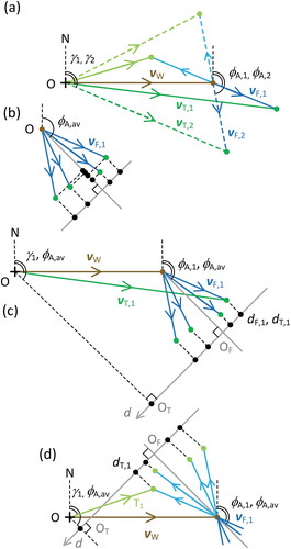
Figure 3. Cluster- and projection-method analyses of large-moth echoes observed at heights of 475 to 625 m between 01.00 and 02.00 h on 14 September 2007. (a) Distribution of track speeds; (b) distribution of track directions; (c) distribution of alignments; (d) formation of along-track (A, dark blue) and back-track (B, light blue) alignment groups and elimination of outliers (grey, also indicated in (a) and (b)); mean directions and the range ±1 SD are shown inside the circle in (b) and (d); (e) track velocity endpoints (green) relative to origin O (larger cross, where insect velocity is zero), and centroid of endpoints (smaller cross); (f) putative-wind velocity endpoints for A and B groups, and centroids (with centroid of selected group circled in red); (g) variation of A and B group RMSs with assumed airspeed, with selected airspeed/group combination circled in red; (h) scatterplot of flight- and track-vector projections onto normal to the mean heading direction, and linear regression fit

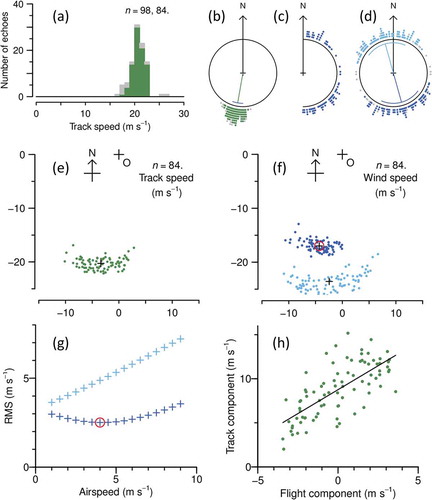
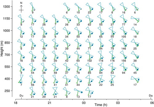
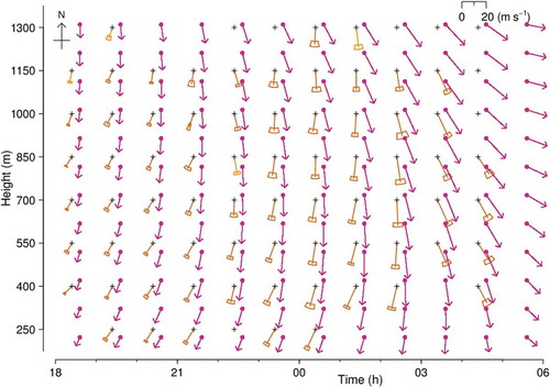
Figure 4. Track directions (green) and alignments (blue) and their SDs, and resolved headings (dots), for large moths at Bourke, NSW, during the night of 13–14 September 2007. Track direction mean and SD represented as in Figure 3(b); length is arbitrary. Alignment represented by hourglass symbol, width of which indicates the ±1-SD range of the alignment distribution. Large dots indicate heading resolved by projection method, blue if p ≤ 0.05 and grey if 0.05 < p ≤ 0.2; small black dots indicate heading closest to track direction. Numbers are sample size for the unit. Key: Du, dusk (end of civil twilight, 18.31 h); Da,dawn (05.53 h). Note: observations ceased at 05.00 h

As the cluster method demonstrated (Figure 1), it is the spread of heading angles that allows the ambiguity to be resolved and the wind vector to be determined. In terms of distances, the spread of φ_A produces the greatest effect along the normal to the mean alignment direction φ_A,av, where it is proportional to the sine of the angle difference φ_A,m,i – φ_A,av, and has the least effect along the mean alignment (cosine of φ_A,m,i – φ_A,av) (Figure 2(b)). The spread of distances along the φ_A,av axis is due also to variation between individuals of the airspeed a_i, an unmeasured quantity; such variations will also affect distances along the normal to the φ_A,av axis, but (provided the angle differences φ_A,m,i – φ_A,av, are not large) to a lesser degree. Thus, distances d along the normal to the φ_A,av axis, i.e. projections of the individual flight vectors onto this direction, d_F,i (Figure 2(c)) provide an efficient representation of the variation in the alignment measurements φ_A,m,i. These distances can be related directly to the two other available measurements, the track speed and track direction, as these too can be projected onto the normal, with values d_T,i (Figure 2(c)). The two projections are calculated as

(7) $d_{\mathrm{F},i}=a_{j}sin\left({\phi }_{\mathrm{A},m,i}-{\phi }_{\mathrm{A},av}\right)d_{\mathrm{T},i}=v_{\mathrm{T},i}sin({\gamma }_{m,i}-{\phi }_{\mathrm{A},av})$(7)

While these distances are measured from different origins (O_F and O_T respectively, (Figure 2(c)) their differences from one insect to the next are identical. Thus, a linear regression of the track projections (dependent variable) against the heading projections (independent variable) should result in a slope of 1.

Now consider the case where the flight vectors are actually along φ_A,m,i + 180° (Figure 2(d)). The track vectors now have a different form, and their projections d_T,i appear in the exact reverse order along the normal direction. As the set of heading directions differs only by a rotation of 180°, the contribution of the flight vectors to the d_T are expected to be of the same size, but with reversed sign. Therefore, a regression of d_T,i against d_F,i, with the latter calculated as previously (i.e. with φ_A,m,i, not φ_A,m,i + 180°), will now have a slope of –1. Thus, if the regression slope is significant, the alignment ambiguity is resolved.

As in the cluster method, a value must be assumed for the airspeed a. The differences of the projection distances d_F and d_T will only be equal, and the regression slopes ±1, if the assumed airspeed matches the insects’ actual airspeeds. However, in this method it is not necessary to try a series of airspeeds until a good match is found. The equations are linear in a, so if a slope b is obtained for an assumed airspeed a_as, the actual airspeed can immediately be estimated as ba_as. Airspeeds of larger migrant insects are typically in the range 3 to 6 ms^–1 (Drake and Reynolds 2012, chapters 6, 9), and 4 ms^–1 has been adopted for a_as in the analyses presented here. With the heading resolved and the airspeed estimated, the methods of the previous section (Equations (3(4) $\stackrel{‾}{}{v}_{\mathrm{P},x,s,j}=\frac{1}{n}\sum _i{v}_{\mathrm{P},x,s,j,i},\overline{v_{\mathrm{P},y,s,j}}=\frac{1}{n}\sum _i{v}_{\mathrm{P},y,s,j,i}.$(4) -6(7) $d_{\mathrm{F},i}=a_{j}sin\left({\phi }_{\mathrm{A},m,i}-{\phi }_{\mathrm{A},av}\right)d_{\mathrm{T},i}=v_{\mathrm{T},i}sin({\gamma }_{m,i}-{\phi }_{\mathrm{A},av})$(7) )) can be employed to estimate the wind speed and direction for each insect and then the averages and standard deviations of these.

2.3. Preliminary procedures

The two methods described above implicitly assume that the insects in the sample being analysed comprise a single (behavioural) population and that all insects in the sample experience the same wind. To obtain samples where these assumptions are approximately valid, datasets of radar observations will need to be partitioned, first by insect class and secondly by time and height. In the dataset from which the examples presented here are drawn, estimates of insect size, shape, and wingbeat frequency, obtained from analyses of individual echo signals, have been used to classify each echo as probably originating from an Australian plague locust (Chortoicetes terminifera), a large moth, or a medium-sized moth (Hao et al. 2020). Samples were then formed from a single insect class. As wind will typically vary with both time and height, and as the radar-observed insect tracks usually exhibit both of these variations, samples need to be drawn from limited time periods and height ranges. For observations from the Australian IMR, the source of the data presented here, sampling periods of duration 1 h and depth 150 m, termed ‘units’ (following Hao, Drake, and Taylor 2019), have proved satisfactory. Some units will produce samples that are too small to obtain a reliable result (see below), but on nights of intense migration there can be more than 50 units with adequate samples. Minor variations of airspeed within an insect class, and of wind within a unit, can be treated in the same way as measurement errors; on occasions when they are larger than usual, fewer units will meet the statistical criterion (e.g. p ≤ 0.05) for confident resolution of the ambiguity.

In the scenarios of Figures 1 and 2, all alignment measurements fall within a range of values that does not extend as far as either the 0° or the 180° limits of the variable φ_A. In these circumstances, it is straightforward to assign the values φ_A,m,i to one set of putative winds and φ_A,m,i + 180° to the other. Very often, however, the range of actual heading angles will extend over one of the limits, and as a result the measured alignments for some insects in the sample will have φ_A values close to 0° (but always positive) and for others φ_A will be close to 180° (but never greater) (see Results for example,). This splitting is artefactual and would lead to some putative winds from each group (– and + in Equation (3)(4) $\stackrel{‾}{}{v}_{\mathrm{P},x,s,j}=\frac{1}{n}\sum _i{v}_{\mathrm{P},x,s,j,i},\overline{v_{\mathrm{P},y,s,j}}=\frac{1}{n}\sum _i{v}_{\mathrm{P},y,s,j,i}.$(4) , and index s there and subsequently) falling into one cluster and the remainder into the other cluster, leading to an unsuccessful or invalid analysis. Appropriate grouping is achieved by first determining the mean alignment direction φ_A,av by the usual method of doubling the angle, calculating the circular mean, and halving the result (Fisher 1993). The φ_A,m,i values are then divided into those that fall within 90° of this direction, and the remainder. One group is then formed by combining the subsets, but with 180° added to the φ_A,m,i of the second subset; the other group is formed similarly, but with the 180° added to the first subset. The result is two well-formed groups, one centred on φ_A,av and the other on φ_A,av + 180°. For consistent identification, it is useful to also calculate the mean track direction γ_av and then denote the group that is centred at an angle closer to this (i.e. <90° from it) as A (‘along-track’) and the other one by B (‘back-track’). As part of this procedure, outliers, identified as insects with any of the measurement values v_T,m,i, γ_m,i, and Ø_A,m,i more than two SDs from their sample means, can be eliminated.

2.4. Precision of the estimates and statistical tests

In the idealized scenario of Figure 1(c), both the difference in spread of the two clusters, and their separation, is obvious. With larger measurement errors, and/or more variation (within the sample) of actual airspeeds and/or of the wind, the clusters (and especially the smaller one) will become broader. If the airspeed is small, the clusters will be closer and may start to overlap; and if the distribution of actual headings is not unimodal, overlapping may again arise but now through incorrect assignment of points to clusters. To determine whether identification of one cluster as the smaller (and ‘correct’) one is likely to be reliable, a statistical test is required. The measure of cluster spread used, the MSS (Equation (5)(5) $S_{s,j}=\frac{1}{n}\sum _i\left[{\left(v_{\mathrm{P},x,s,j,i}-\overline{v_{\mathrm{P},x,s,j}}\right)}^2+{\left(v_{\mathrm{P},y,s,j,i}-\overline{v_{\mathrm{P},y,s,j}}\right)}^2\right]$(5) ), has a form close to that of a variance, and the ratio of the – and + MSSs for the same sample is thus similar to an F statistic (the ratio of two variances, larger over smaller). The conventional F-test for comparing variances (e.g. Sokal and Rohlf 2012) has therefore been employed. As either cluster could be the ‘correct’ one, a two-tailed probability criterion applies. The sample sizes n are the same for numerator and denominator, so the number of degrees of freedom is 2n – 2, this being the number of x coordinates plus the number of y coordinates less the two averages calculated from these. p-values calculated in this way (denoted p_F) appear consistent with qualitative assessments made from plots of the two clusters. The heading is resolved if the p-value is sufficiently low; as well as the usual p ≤ 0.05 criterion, a less demanding p ≤ 0.2 requirement has been investigated.

For the projection method, normal regression-analysis criteria can be employed: if the p-value for the slope b (denoted p_b) exceeds 0.05 (or 0.2), the ambiguity is not resolved. For both methods, uncertainties for the sample v_W and φ_W estimates can be obtained by dividing the SDs of these quantities, calculated from the individual putative winds (see above), by $\sqrt{n}$. For the cluster method, the root-mean-square (RMS) deviation of the selected cluster, $\sqrt{S_{s,J}}$, provides an additional general measure (with unit ms^–1) of the precision of the estimates. It is expected that, if the result of the F-test is significant, this will be smaller than the airspeed estimate a_J.

2.5. Limitations

The most obvious limitation is that a minimum number of insects is required in each unit, so the method will only work when migrations are moderately intense. Units could be extended, in both duration and height range, to increase sample sizes, but only for periods when both the wind and migratory behaviour are relatively steady; this will, of course, lead to the information provided having poorer temporal and vertical resolution. More fundamentally, the methods depend on the assumption that the headings are clustered around a single direction. If there are in fact two or more populations heading in different directions, a compact cluster will not form and the methods will fail. Riley and Reynolds (1986) document some obviously bimodal distributions of the φ_A,m,i, but mixed populations (and more particularly mixed behaviours by a single population) may not always be immediately evident; for example, if the headings are almost opposite, the two alignment distributions will superimpose. Another possible problem is that the distribution of φ_A,m,i could be close to uniform, the difficulty then being not with the core procedures but at the preliminary stage of assigning points to the two groups A and B. The Rayleigh test of non-uniformity (Fisher 1993), with angle doubling, can be used to determine whether there is enough directionality in the alignments for an analysis to be viable. Finally, the distribution of headings could be so narrow that the ‘correct’ cluster is very spread out (in one dimension) as the insect flights (F in (Figure 1(a)) are almost parallel. The heading will still be resolved, but the inferred wind direction will have poor precision.

2.6. Implementation

The methods have been implemented in R (R Core Team 2020), with the R package ‘Circular’ (Agostinelli and Lund 2017) used to calculate statistics of angular quantities. The R scripts use standard summary files produced by the IMR processing system as input. A variant that analyses data from a newer, upgraded radar (Drake et al. 2020) has also been developed.

2.7. Simulations

The effectiveness of the methods has been investigated through simulation. The primary aim was to establish whether the methods work well for all angles between heading and track, because if this is not the case a biased representation of the insects’ behaviours will result. Simulation also allows the sensitivity of the methods to be determined, and their effectiveness when sample sizes are small, or airspeeds are low, to be assessed. In addition, a good correspondence between outputs from simulated and real data provides a degree of verification of the model underlying the methods and its implementation in equations and code.

The simulations were made in R, using a specially developed script that generates samples of ‘insects’ (i.e. headings, plus the track speeds and directions calculated for flight at a given airspeed and in a given wind) and then analyses them by both the cluster and the projection methods. All generated quantities are subject to random variation representing behavioural differences in headings and airspeeds, variability in the wind, and measurement errors. Random distributions have Gaussian form except in the case of heading directions when the von-Mises (‘circular normal’) distribution is used as this quantity varies over a broader range. Input parameters are mean wind speed, spread of wind speed, spread of wind direction, spread of headings (expressed as the von Mises parameter κ), mean airspeed, spread of airspeed, and measurement errors for track direction and track speed. The mean direction of the wind is fixed:it is set to blow towards 90° (i.e. E). The heading direction is varied through 360° at 30° intervals starting at 10°. The same set of generated values are used for the cluster and projection analyses, but new random distributions are used for each heading angle. The programme performs 100 replicate sets of calculations and calculates statistics of the results, and repeats this for a series of different sample sizes n_s and airspeeds a. As the aim has been to determine the robustness and limits of the method, performance has been assessed at both p ≤ 0.05 and p ≤ 0.2 and samples sizes as low as 6.

Parameters have been chosen to represent an individual unit from the night of 13–14 September 2007, with airspeed, spread of headings, wind speed, and the spread of wind direction and speed, obtained from the analysis of this unit (see Results). For measurement uncertainties on track speed and direction and on heading direction, we drew on estimates of about 0.2 ms^–1, 2° and 1° respectively by Harman and Drake (2004) and of 1%, 1°, and 1° by Smith, Riley, and Gregory (1993), and also noted differences of up to 5 ms^–1 when track speeds are measured in different ways (Drake and Reynolds 2012, their Figure A7). Taking account also of the spread of measured values for a unit, which sets an upper limit, we adopted values of 0.5 ms^–1 for track speed and 2° for track direction; the spreads of wind speed and wind direction were reduced by these amounts. As uncertainties for the heading direction are small compared with the spread, they were not explicitly modelled. The spread of airspeeds was set to 25% of the airspeed value; this range was chosen to represent the considerable variation in individual size and physiological condition typically found within a population.

2.8. Example datasets

We demonstrate the effectiveness of the two methods by applying them to data obtained from the IMR located at Bourke Airport, New South Wales (30.0415° S, 145.9523° E), in the inland plains of eastern Australia, during September and October 2007. During this period, there was a series of high-intensity night-time flights of insects of the large-moth type. Detailed results are provided for the night of 13–14 September 2007, when the migration was particularly intense and extended through both the 175 to 1350 m height range of radar coverage and the 11 h of radar observations. Only echoes falling into the large-moth class are included in the samples. Some more general results are provided for a larger dataset comprising the 15 nights in September and October 2007 with the most large-moth echoes. This includes movements in different directions and at different speeds, and so provides a more varied test of the new analysis methods. Analysis of a unit was attempted if there were at least six fully analysable echoes left after removal of outliers, and the heading was determined to be resolved if the projection-method b (slope) parameter was significantly different from zero at the p ≤ 0.2 level. These criteria were deliberately set low, in order to establish how broadly the methods can be employed.

Wind estimates from meteorological observations, used here to verify the winds inferred from the radar observations, were obtained from European Centre for Medium-Range Weather Forecasts (ECMWF) reanalyses (ECMWF 2018) and dynamically downscaled using The Air Pollution Model (TAPM) (Hurley 2008; Hurley, Edward, and Luhar 2008; Hao, Drake, and Taylor 2019). For ready comparison with the insect tracks and flight vectors, wind directions are presented here as the direction the wind is blowing towards. TAPM produces hourly averaged winds for a series of heights through the 150 to 1350 m range of the radar observations. The wind for a specific unit was obtained by calculating E and N components of the wind vectors immediately above and below the unit’s centre-height and interpolating them linearly to the centre height. Interpolation in time was not required as the meteorological and radar hourly intervals corresponded.

3. Results

3.1. Single unit

An example of the methods applied to a single unit is illustrated in Figure 3. The sample is for large moths observed between 01.00 and 02.00 h on 14 September 2007 between the heights of 450 and 600 m. The distributions of the measured track speeds, track directions, and alignments are shown in (Figure 3(a-c)). The alignments (Figure 3(c)) are evidently split artefactually at the 0° and 180° limits of this quantity. The output of the preliminary procedure to form two groups of possible headings, and remove outliers, is shown in Figure 3(d). The two groups contain 84 insects, with headings centred on directions 164° and 344°, respectively; the first of these, being closer to the mean track direction of 190°, is designated A and the second B. The heading distributions are broad (angular SD 38°) in comparison to the track directions (10°).

The distribution of track-vector endpoints (green dots in Figure 1) and the A and B sets of putative-wind endpoints (blue dots), calculated for an assumed airspeed of 4.0 ms^–1, are shown in Figure 3(e,f). All three endpoint clusters are elongated across the mean track direction, indicating greater variation arising from directional factors (principally the spread of alignments, but variation in wind direction, track direction measurement error, and heading measurement error will also contribute) than from speeds (variation in wind speed and airspeed, and track speed measurement error). The A and B clusters are well separated, with A somewhat smaller than the cluster of track endpoints and B clearly larger. An arc form, like that in Figure 1(c), is also evident in the B cluster. RMSs are 3.3 ms^–1 for the tracks, 2.5 ms^–1 for A and 4.9 ms^–1 for B; F is 3.78, there are 166 degrees of freedom, and p < 0.001. The variation with assumed airspeed of the RMSs for the A group exhibits a clear minimum at 4 ms^–1 while that of the B group increases monotonically and is consistently higher (Figure 3(g)). The A group is therefore selected as the heading direction. The inferred wind speed is 17.5 ms^–1, towards direction 194° (Figure 3(f)). The individual inferred winds in the A group have spreads of 0.9 ms^–1 (SD) in speed and 7.7° (circular SD) in direction.

For the projection method, Figures 3(a-d) apply, except that only the A set of alignments (Figure 3(d)) is required. Projections along the normal to the mean heading direction (164°), calculated from Equation (7)(7) $d_{\mathrm{F},i}=a_{j}sin\left({\phi }_{\mathrm{A},m,i}-{\phi }_{\mathrm{A},av}\right)d_{\mathrm{T},i}=v_{\mathrm{T},i}sin({\gamma }_{m,i}-{\phi }_{\mathrm{A},av})$(7) with a_as = 4 ms^–1, are plotted in Figure 3(h) along with the regression of the track-vector projection on the flight-vector projection. The slope b is 1.09 ± 0.12, p < 0.001, with a coefficient of determination R² of 0.51 (indicating 51% of the variance is explained), and the RMS for the residuals is 2.1 ms^–1. The corrected airspeed ba_as is therefore 4.3 ms^–1; a check reanalysis with a_as set to this value gave the expected b value of 1.00.

3.2. Single night

Results for the night of 13–14 September 2007 (from 18.00 to 05.00 h, UTC+10) are summarized in Table 1 for both methods, and for the projection method are presented in Figure 4. The requirement of at least 6 good-quality large-moth echoes was met by 79 of the 88 units. Migration was sustained throughout the hours of darkness (19.00 to 05.00 h), with moths flying at all altitudes receiving radar coverage (150 to 1350 m). The heading was resolved at the p ≤ 0.05 probability level in 67 (85%) of the 79 analysed units, and a further 4 units were resolved at p ≤ 0.2. Some units with < 10 echoes were resolved at p ≤ 0.05, and only one of the 54 units with ≥ 20 echoes failed to resolve at this level. There are no ‘flips’ (changes of approximately 180° from one unit to the next, indicative of a probable incorrect resolution). All headings are resolved as along-track (group A, within 90° of the mean track direction), and therefore on this occasion the common practice of resolving the heading ambiguity by selecting the direction closer to the track direction (black dots in Figure 4) is validated. Headings were consistently towards the S or SE (mean 145°, SD 14°; 0.05 < p ≤ 0.2 cases included), showed little variation with either time or height, and were always to the left of the track, at angles ranging from 0° to 76°; this difference decreased later in the night when tracks turned more to the SE. Estimated representative airspeeds range from 2.2 to 7.8 ms^–1 (average 4.1 ms^–1).

Table 1. Performance of different heading-resolution methods

Method	Units analysed n, (%)	Cluster n, (%)	Projection n, (%)	Subtraction n, (%)	Putative n, (%)
Night of 13–14 September 2007
Units resolved	79, (100)	60, (76)	67, (85)	30, (38)	25, (32)
along-track	79, (100)	60, (76)	67, (85)	13, (16)	9, (11)
back-track	0, (0)	0, (0)	0, (0)	17, (22)	16, (20)
15 nights, September and October 2007.
Units resolved	845, (100)	607, (72)	627, (74)	349, (41)	210, (25)
along-track	845, (100)	607, (72)	620, (73)	324, (38)	186, (22)
back-track	0, (0)	0, (0)	0, (0)	25, (3)	24, (3)
6 ≤ nu ≤ 12	279, (33)	162, (58)	150, (54)	128, (46)	84, (30)
12 < nu ≤ 25	311, (37)	227, (73)	236, (76)	138, (44)	72, (23)
25 < nu ≤ 50	195, (23)	165, (84)	181, (93)	69, (35)	39, (20)
50 < nu ≤ 100	54, (6)	47, (87)	54, (100)	14, (26)	13, (24)
nu > 100	6, (1)	6, (100)	6, (100)	0, (0)	2, (33)

Note. At p ≤ 0.05. The ‘Units analysed’ column also gives the number of units resolved by the assume-along method. See main text (below) for description of this and of the subtraction and putative methods. Percentages are proportions of the total number of units (79 for the night of 13–14 September and 845 for the 15 nights), except at bottom-right where they are proportions of the number of units in the sample-size class (leftmost two columns).

The winds inferred from these analyses are shown in Figure 5, along with the winds determined from meteorological observations via TAPM. Both sets of winds show a coherent pattern, generally similar in their forms and to the pattern of the tracks in Figure 4. The two wind sets show an increase in speed during the course of the night, and all three direction sets show a change in direction, from SSW to SE, and a slight anticlockwise (eastward) rotation with height. Comparison of Figures 4 and 5 indicates that the radar-derived winds are directed slightly clockwise (westward) of the tracks, as is to be expected given that track speeds (range 10 to 24 ms^–1) were considerably faster than the 4 ms^–1 airspeeds and the resolved heading directions (Figure 4) were consistently to the SE. The RMS difference between the two sets of wind vectors is 4.9 ms^–1 (for 71 units), or 3.0 ms^–1 in speed and 15° in direction. For the difference between the measured track vectors and the TAPM winds, the RMSs are smaller: 3.3 ms^–1 (for 79 units), or 1.6 ms^–1 in speed and 9° in direction.

Figure 5. Wind speeds and directions inferred from projection-method analyses of large-moth echoes (orange, paler for units with 0.05 < p ≤ 0.2) and from dynamic downscaling of meteorological observations via TAPM (violet), for the night of 13–14 September 2007 at Bourke, NSW. Boxes at end of large-moth inferred-wind arrows indicate ±1-SD ranges of individual wind speed and direction estimates. Number of echoes in each unit as in Figure 4

3.3. Multiple nights

For the 15-night dataset, there were 845 units with 6 or more large-moth echoes after elimination of outliers. Of these, 607 (72%) resolved the heading at p ≤ 0.05 using the cluster method, and 627 (74%) using the projection method (Table 1), with all selecting group A (along-track). At the less demanding p ≤ 0.2 level (not tabulated), the number of units resolved rose to 717 (85%) for the cluster method and 724 (86%) for the projection method, with two units classified as back-track and the remainder as along-track for both methods. Resolution rate increased with the number of insects in the unit, n_u, from a little over 50% for 6 ≤ n_u ≤ 12 to 100% for n_u > 100 (Table 1).

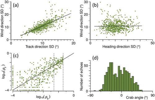
After eliminating a small number of outliers, the SD of heading directions within a unit averaged 20° over the 15 nights; for track directions and inferred-wind directions the SD averaged 10° and 11° respectively. For track speeds and inferred-wind speeds, the average unit SDs were 1.2 ms^–1 and 1.1 ms^–1 respectively. There was a strong relationship between the spread of track directions within a unit, and the spread of the inferred-wind directions (slope 1.09 ± 0.03, p < 0.001, R² = 0.60; Figure 6(a)), and similarly with track and inferred-wind speeds (slope 0.86 ± 0.02, p < 0.001, R² = 0.81; not shown). However, there is no equivalent relationship between the spread of heading directions and the spread of wind directions (slope 0.01 ± 0.02, p = 0.65, R² < 0.01; Figure 6(b)). Larger spreads in heading directions are weakly associated with larger spreads in track directions (slope 0.16 ± 0.01, p ≤ 0.001, R² = 0.15; not shown). p-values for the two methods, after logarithmic transformation, are linearly related, though not closely (Figure 6(c)). p_F is lower than p_b (but ≥ 0.0001) in 36% of units, and the reverse is true in another 33%; in the remaining units (31%), both p-values are < 0.0001. The ‘crab angle’ (χ = φ – γ, the angle the insect is heading to left (–ve) or right (+ve) of its track, ranges from – 60° to +60° (Figure 6(d)).

Figure 6. Features of the analysis results for 15 nights of intense large-moth migration at Bourke, NSW, in September and October 2007, for units with the heading resolved at p ≤ 0.2. (a), (b) Relation of the SD of the inferred wind direction to the SD of the measured track (a) and heading (b) directions, n = 716 (after elimination of 8 units with outlier SDs); solid lines indicate regression fits. (c) Relation of p-values (logarithmically transformed) of the cluster (p_F) and projection (p_b) methods, n = 498 (with units with both p-values < 0.0001 excluded); solid line indicates equal p-values, dashed lines indicate p = 0.05 (left) and p = 0.2 (right). (d) Histogram of crab angle χ, n = 724

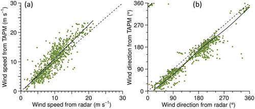
The winds inferred from the radar observations over the 15 nights exhibited a wide range of speeds and directions but were generally consistent with winds estimated for the same time and height from meteorological observations (Figure 7). A regression analysis for wind speeds indicated the TAPM winds were slightly faster than the radar winds (slope 1.15 ± 0.02, p < 0.001, R² = 0.77, residual 2.4 ms^–1, n = 724). After eliminating 6 units as outliers (direction differences >90°), the radar wind directions have an average offset of 20° clockwise from the TAPM winds and an SD of 19° about this mean. The circular correlation coefficient is 0.97 (p < 0.001), and a circular-circular regression fits the points well (Figure 7).

Figure 7. Relation of wind estimated from radar observations of insects to wind from meteorological observations downscaled via TAPM. Data from 15 nights as in Figure 6, n = 724 for speeds (a) and 718 for directions (b). Dashed line indicates where the two quantities are equal, solid line is regression fit (linear in (a), circular-circular in (b))

3.4. Comparison with alternative methods

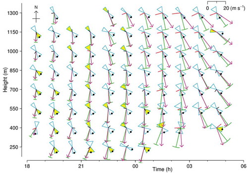
Summaries of the performances of three previously used methods are included in Table 1. The ‘assume-along’ method simply selects whichever of the two possible heading directions is closer to the track direction. The ‘subtraction’ and ‘putative’ methods are methods B and C of Hao, Drake, and Taylor (2019); both make use of winds estimated from meteorological analyses. The assume-along method can be applied to any unit for which a mean track and heading can be calculated, so its resolving rate for the samples considered here is 100% and, by definition, it always resolves as along-track. Detailed results for the night of 13–14 September 2007 are shown in Figure 4 for the assume-along and projection methods and in Figure 8 for the assume-along and subtraction methods. The wind-based methods perform poorly on this night’s data. Although track, heading, and wind directions all vary smoothly, both through the night and with height, and the variations are not large, the heading is resolved only for a minority of units and switches from along-track initially to predominantly back-track between 21 and 23 h (Figure 8). There are a few flips, with no associated sudden change in heading, track or wind. Very few of the inferred flight vectors fall within one SD of the observed heading, and their average speed varies, increasing from1.5 ms^–1 before 21 h to 4.9 ms^–1 after 01 h. This night appears to have been particularly unfavourable for the wind-based methods, as in the 15-night sample the great majority of units that are resolved are along-track, like those resolved by the new methods (Table 1). Nevertheless, resolution rates for the wind-based methods are around half those of the new methods, which exceed 70% (Table 1).

Figure 8. Resolution of heading direction by assume-along and subtraction methods, for same dataset as that of Figures 4 and 5 (and using same symbols). Key: blue, alignment and its SD; green, track vector and its SD; violet, TAPM wind vector (interpolated to mean height for unit); red or black without arrowhead, flight vector (heading and airspeed) inferred by vector subtraction; black dot,heading resolved by assume-along method; yellow fill,heading resolved by subtraction method. For visibility, flight vectors with speeds < 3 ms^–1 are shown as 3 ms^–1 and coloured black instead of red

3.5. Simulations

Parameters for the simulations were set from values obtained in the analysis of the unit at 02 h (start time) and 1000 m in Figure 4, this being preferred to the unit in Figure 3 because the p-values obtained were higher (i.e. inference was less strong) so that limitations of the methods are more evident. The measured spread of heading directions for this unit was 34°, the inferred wind speed (from a cluster-method analysis) was 18 ms^–1, and the spreads of inferred wind directions and speeds were 14° and 2.5 ms^–1 respectively. For the simulations, these last two quantities were reduced to 12° and 2 ms^–1 to take account of measurement uncertainties (see Materials and Methods).

A typical set of simulation results is shown in Figure 9, these being for a simulated airspeed of 4 ms^–1. When analysed with the cluster method, the simulation shows no significant variation of the p-value with the heading direction (Figure 9(a)), and in consequence no variation of the ability to resolve the heading ambiguity (Figure 9(b)). As expected, p-values decrease as sample size n_s increases, and for n_s = 6 the conventional p ≤ 0.05 criterion is not usually met, though around 60% of replicates are resolved at p ≤ 0.2. For the projection method, there is a clear variation of p-values with heading direction for all four sample sizes (Figure 9(c)). For the smaller sample sizes, this produces a similar variation in the proportion resolved but this is absent for the largest sample and slight for the sample of 25, because in these cases p ≤ 0.2 for almost all the replicates. For the larger samples, the p-values for the projection method are lower than those for the cluster method, but for the smallest sample this difference is reversed. For n_s = 55, 25, and 12, there are no replicates in which the heading appears to be resolved (at either p ≤ 0.2 or p ≤ 0.5), but the incorrect assignment is made. For n_s = 6, incorrect assignments are made for about 1% of replicates at p ≤ 0.2 and 0.1% at p ≤ 0.05.

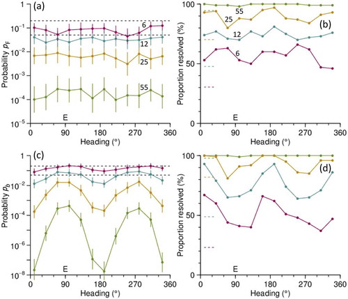
Figure 9. Simulation results for unit at 02 h (start time) and 1000 m on 14 September 2007 and an airspeed of 4 ms^–1, showing variations with heading angle and sample size. E indicates the 90° direction (towards E) of the simulated wind. Samples sizes n_s were 55 (as in actual unit, after removal of outliers), 25, 12 and 6. (a) Mean (point) and standard error on the mean (bars) over 100 replicates for F-test p-value from cluster-method analyses. Dashed lines indicate p = 0.2 and p = 0.05. (b) Proportion of the 100 replicates resolved by the cluster method at p ≤ 0.2. Short dashed lines indicate average over the 12 heading directions for the proportion resolved at p ≤ 0.05. (c), (d) Same as (a), (b) for projection method; p-value is now that for the regression slope parameter b.

Airspeeds estimated by the two methods are broadly consistent (RMS difference 0.4 ms^–1 for n_s = 55, rising to 0.8 ms^–1 for n_S = 6) and agree well with the input value of 4 ms^–1 when n_s = 55 but increasingly produce overestimates when the sample is smaller, by as much as 40% (average) for n_s = 6. This can be understood as due to lower airspeeds reducing the probability of resolution, so higher airspeeds are over-represented in the averaged sample. For the smaller sample sizes, there are also peaks in the estimated airspeed, more pronounced in the projection method, in the downwind and upwind directions, and corresponding peaks and troughs are present in the estimated wind speeds. The estimated wind directions are accurate when the heading is downwind and upwind, but for smaller sample sizes there is a bias when it is to left or right of the wind; however, this only reaches 6° (average) in the worst case (with n_s = 6) and, like the speed biases, is insignificant for samples of 25 or more.

Simulations with different mean airspeeds show that the effectiveness of both methods falls rapidly as the airspeed is reduced (Figure 10). If 50% of units being resolved (and resolved correctly) is taken as a criterion for the methods to remain useful, then for an airspeed of 3 ms^–1 around 10 insects are required in each unit and for 2 ms^–1 around 20 are required. With these numbers, the proportion of incorrect assignments remains below 5%. At airspeeds below 2 ms^–1, too few units are resolved for the methods to have any utility. There is little to choose between the two methods in terms of their performances at different airspeeds.

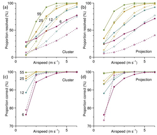
Figure 10. Simulation results for airspeeds in the range 1 to 6 ms^–1, for same unit and sample sizes as in Figure 9. (a), (b) Proportion of units resolved by cluster method and projection method. (c), (d) Proportion of units resolved by these two methods for which the assignment is correct. Results at p ≤ 0.2 indicated by solid lines, at p ≤ 0.05 by dashed lines

4. Discussion

The ability of entomological radars to measure the alignment of migrating insects accurately and precisely, but not to be able to resolve the 180° heading ambiguity, has long frustrated confident interpretation of the observations of insect orientation produced by these systems. The usual approach has been to assume that the insects orient along their track, so the direction within ±90° of the track is selected as the heading. When the insects are grasshoppers, use of this assumption is supported by the early study of Riley and Reynolds (1986) in which vertical-beam and scanning radar observations were made simultaneously, with the scanning system used to provide accurate wind data by tracking a pilot balloon. In more recent studies, measured track speeds that exceed wind speeds estimated from meteorological observations by a few metres per second provide support for the assumption, but as demonstrated here (Figure 8 and see below) these speed differences may not be reliable. The analyses presented in this paper demonstrate that the along-track assumption is valid for the large moths that were migrating over Bourke during September and October 2007. However, alignments at a large angle to the track have been recorded with other insect types, and then the choice of one heading over the other starts to appear arbitrary; and indeed, use of the assumption can then lead to flips (Hao, Drake, and Taylor 2019). The simulation analyses presented here indicate that the new approach, especially the cluster-method variant, should resolve these cases reliably. This is the subject of ongoing research, focused particularly on the orientation behaviour of Australian plague locusts during their nocturnal migrations.

For the new methods described here to work, the insect population needs to have a high enough airspeed and a sufficient spread of heading directions, and the radar needs to have sufficient measurement precision for the resulting variations in track direction and speed, which are usually quite small, to be detectable. The example analyses presented here demonstrate that these requirements are met for the Bourke IMR when it is observing large insects with airspeeds of about 4 ms^–1, and the simulations suggest it may have utility at airspeeds as low as 2 ms^–1. Exploratory analyses, not presented here, indicate that the effectiveness of the new methods is not confined to insects of the large-moth type. In broad terms, the methods work for ‘strong-flying’ insects, i.e. those with airspeeds sufficient to make a non-negligible contribution to their flight trajectory (rather than just being carried along on the wind). The ability of the two methods to resolve the heading for the majority of units with > 12 insects, and the absence of flips, suggests the results are robust. This is in contrast to the two wind-based methods (subtraction, putative) proposed previously, which, despite apparently adequate samples, exhibited both flips and periods when units could not be resolved. The sometimes-poor performance of the wind-based methods is very likely due to systematic errors arising from the different origins of the track and wind data, and the often-small size of the difference of these two vectors relative to their magnitudes. Winds within about 1 km of the surface are particularly difficult to estimate because they are strongly affected by any nearby terrain features, and by the thermal and roughness properties of the ground itself. There may of course also be inaccuracies in the radar data. In the new methods, all data originate from a single source, the radar, and only one speed is measured. Systematic errors, if present, will carry through to the estimated values of the airspeed and the inferred wind, but will have little effect on resolution of the heading as they will be similar for each insect in the sample.

The simulations incorporate many parameter values that are not well established and that are likely to vary in different circumstances, and they also examine only one wind-speed value and one value for the spread of heading directions. The encouraging results obtained should therefore be regarded as indicative rather than conclusive. They clearly demonstrate that both methods work for insects moving in all directions relative to the wind, though there is some potential for directional bias. As expected, they work better for larger samples, and for the smallest sample size n_s of 6 insects they are effective for only about 25% of units at p ≤ 0.05 and about 50% at p ≤ 0.2. The projection method is more effective at resolving headings at right angles to the wind than headings that are down- or upwind, but for larger samples this is not a problem as all probability levels are well below the p ≤ 0.05 criterion likely to be adopted in most applications. However, use with small samples is very desirable as this allows investigations of less intense migrations, and therefore the cluster method appears to be the more useful of the two. Its assessment of cluster size in two orthogonal directions may account for its effectiveness hardly varying with the angle between heading and wind. The simulations also indicate that it produces lower p-values than the projection method when samples are small, and this leads to more of these units resolving; however, the total resolution rate is slightly lower than that of the projection method (Table 1). As the projection-method algorithm does not need to test a series of different airspeed values, it is simpler and requires less computation than its cluster counterpart, but with modern data-processing technology these advantages are of little importance. Although the cluster method is less prone to bias, estimated airspeeds and inferred winds can exhibit some variation with the angle of the heading relative to the wind, and in work where the accuracy of these values is important, a correction, taking account of sample size, would need to be incorporated.

Use of the p ≤ 0.2 criterion increased the proportion of large-moth units that were resolved from about 73% to about 85%, but resolved two units as back-track: from the complete absence of back-track units at p ≤ 0.05, it seems likely that these were misidentifications. In many circumstances, the resolved heading directions will form a clear pattern (e.g. Figure 4), and rare outliers are then easily identified (as flips). Use of the less demanding criterion would then allow considerably more information to be reliably extracted from the available data.

How well the methods will work on any given occasion depends on the observing equipment being used (specifically, on how precisely it measures the track direction and speed and the heading), the variability of the wind within the period and height range from which the sample is obtained, the airspeed of the insects and the spread of their orientations, and the intensity of the migration (which determines the sample size). Some caution is therefore needed when comparing behaviours observed in different conditions, or with different radars. However, resolution of the heading direction should still be clear; it is rather the rates at which confident resolutions can be made that will change. The method also depends on the migrants having a unimodal distribution of heading directions. Failure of the method to resolve the heading ambiguity in conditions when simulations suggest it should be able to do so may be a useful indicator of a bimodal or more complex heading distribution.

While the main purpose envisaged for these methods is the resolution of the heading-direction ambiguity, they also provide estimates of airspeeds and winds. The former adds a further character of potential value in target identification and can be incorporated into trajectory calculations, replacing an assumed value with an empirical one. During intense migrations, a comprehensive set of boundary-layer wind estimates is obtained (e.g. Figure 5). In the limited comparison presented here (Figures 5,7), there is good general agreement of values and trends. Migrating insects are certainly not always present in the boundary layer, but in warmer climates migrations are not uncommon. Are there locations or circumstances where these methods could function as a wind-finding technique for meteorologists?

5. Conclusions

The new methods of resolving the heading-direction ambiguity presented here are effective when applied to insects with airspeeds of about 2 ms^–1 or greater and are subject only to minor biases. They should therefore be adopted in preference to existing assume-along and wind-based methods when the migrants are larger, ‘strong-flying’, insects. The cluster method appears the better of the two as it resolves more units, and is less prone to bias, when sample sizes are small. Application to larger datasets, especially if these include slower-flying species and insects that orient at large angles to their track, will provide further verification of the validity and effectiveness of the new methods, and a clearer indication of their limitations.

Data availability

The unit analyses for large moths and the TAPM wind estimates presented in Figures (4-8) are provided in the supplemental material. An R script implementing the two methods, and a sample data file containing the data for Figure 3, are also provided.

Acknowledgements

Several former students and technical staff of the School of Science, UNSW Canberra, contributed to the development of the Bourke IMR and its associated data-processing systems, with funding from the Australian Research Council and UNSW Canberra. Dr J. R. Taylor assisted with TAPM wind estimation. Bourke Shire Council provided a site for the radar, and the Australian Plague Locust Commission supported its operation and maintenance. ZH is funded through European Research Council Advanced Grant 741298 (to EW).

Disclosure statement

No potential conflict of interest was reported by the authors.

Supplementary material

Supplemental data for this article can be accessed here.

Additional information

Funding

European Research Council [Advanced Grant / GAP-741298];

References

- Adden, A. 2020. “There and Back Again: The Neural Basis of Migration in the Bogong Moth.”PhD diss., Lund University, Sweden. ISBN: 978–91–7895–382–0.
- Agostinelli, C., and U. Lund. 2017. “R Package ‘Circular’: Circular Statistics (Version 0.4-93).” URLhttps://r-forge.r-project.org/projects/circular/
- Chapman, J. W., J. R. Bell, L. E. Burgin, D. R. Reynolds, L. B. Pettersson, J. K. Hill, M. B. Bonsall, and J. A. Thomas. 2012. “Seasonal Migration to High Latitudes Results in Major Reproductive Benefits in an Insect.” Proceedings of the National Academy of Sciences 109: 14924–14929. doi: 10.1073/pnas.1207255109.
- Chapman, J. W., R. L. Nesbit, L. E. Burgin, D. R. Reynolds, A. D. Smith, D. R. Middleton, and J. K. Hill. 2010. “Flight Orientation Behaviors Promote Optimal Migration Trajectories in High-Flying Insects.” Science 327 (5966): 682–685. doi: 10.1126/science.1182990.
- Chapman, J. W., D. R. Reynolds, and A. D. Smith. 2003. “Vertical-Looking Radar: A New Tool for Monitoring High-Altitude Insect Migration.” BioScience 53 (5): 503–511. doi: 10.1641/0006-3568(2003)053. [0503:VRANTF]2.0.CO;2.
- Chapman, J. W., D. R. Reynolds, K. Wilson, and M. Holyoak. 2015. “Long-Range Seasonal Migration in Insects: Mechanisms, Evolutionary Drivers and Ecological Consequences.” Ecology Letters 18 (3): 287–302. doi: 10.1111/ele.12407.
- Drake, V. A. 1983. “Collective Orientation by Nocturnally Migrating Australian Plague locusts, Chortoicetes terminifera(Walker) (Orthoptera: Acrididae): A Radar Study.” Bulletin of Entomological Research 73 (4): 679–692. doi: 10.1017/S0007485300009287.
- Drake, V. A. 1984. “The Vertical Distribution of Macro-Insects Migrating in the Nocturnal Boundary Layer: A Radar Study.” Boundary-Layer Meteorology 28 (3–4): 353–374. doi: 10.1007/BF00121314.
- Drake, V. A., and A. G. Gatehouse, edited by. 1995. Insect Migration: Tracking Resources through Space and Time. Cambridge, UK: Cambridge University Press.
- Drake, V. A., S. Hatty, C. Symons, and H. Wang. 2020. “Insect Monitoring Radar: Maximizing Performance and Utility.” Remote Sensing 12 (4): 21. article 596. doi: 10.3390/rs12040596.
- Drake, V. A., and D. R. Reynolds. 2012. Radar Entomology: Observing Insect Flight and Migration. Wallingford, UK: CABI.
- Dreyer, D., B. Frost, H. Mouritsen, A. Gunther, K. Green, M. Whitehouse, S. Johnsen, S. Heinze, and E. Warrant. 2018. “The Earth’s Magnetic Field and Visual Landmarks Steer Migratory Flight Behavior in the Nocturnal Australian Bogong Moth.” Current Biology 28 (13): 1–7. doi: 10.1016/j.cub.2018.05.030.
- ECMWF. 2018. “Browse Reanalysis Datasets.” Accessed 2018. https://www.ecmwf.int/en/forecasts/datasets/browse-reanalysis-datasets
- Fisher, N. I. 1993. Statistical Analysis of Circular Data. Cambridge, UK: Cambridge University Press.
- Green, M., and T. Alerstam. 2002. “The Problem of Estimating Wind Drift in Migrating Birds.” Journal of Theoretical Biology 218 (4): 485–496. doi: 10.1006/jtbi.2002.3094.
- Hao, Z., V. A. Drake, and J. R. Taylor. 2019. “Resolving the Heading-Direction Ambiguity in Vertical-Beam Radar Observations of Migrating Insects.” Ecology and Evolution 9 (10): 6003–6013. doi: 10.1002/ece3.5184.
- Hao, Z., V. A. Drake, J. R. Taylor, and E. Warrant. 2020. “Insect Target Classes Discerned from Entomological Radar Data.” Remote Sensing 12 (4): 18. article 673. doi 10.3390/rs12040673.
- Harman, I. T., and V. A. Drake. 2004. “Insect Monitoring Radar: Analytical Time-Domain Algorithm for Retrieving Trajectory and Target Parameters.” Computers and Electronics in Agriculture 43 (1): 23–41. doi: 10.1016/j.compag.2003.08.005.
- Hu, G., K. S. Lim, N. Horvitz, S. J. Clark, D. R. Reynolds, N. Sapir, and J. W. Chapman. 2016a. “Mass Seasonal Bioflows of High-flying Seasonal Migrants.” Science 354 (6319): 1584–1587. doi: 10.1126/science.aah4379.
- Hu, G., K. S. Lim, D. R. Reynolds, A. M. Reynolds, and J. W. Chapman. 2016b. “Wind-Related Orientation Patterns in Diurnal, Crepuscular and Nocturnal High-Altitude Insect Migrants.” Frontiers in Behavioral Neuroscience 10: 8. article 32. doi: 10.3389/fnbeh.2016.00032.
- Huestis, D., A. Dao, M. Diallo, Z. L. Sanogo, D. Samake, A. S. Yaro, Y. Ousman, et al. 2019. “Windborne Long-Distance Migration of Malaria Mosquitoes in the Sahel.” Nature 574 (7778): 404–408. doi: 10.1038/s41586-019-1622-4.
- Hurley, P. 2008. “TAPM V4. Part 1: Technical Description. CSIRO Marine and Atmospheric Research Paper No. 25.” Melbourne: CSIRO Australia.
- Hurley, P., M. Edward, and A. K. Luhar. 2008. “TAPM V4. Part 2: Summary of Some Verification Studies. CSIRO Marine and Atmospheric Research Paper No. 26”. Melbourne: CSIRO Australia.
- Johnson, C. G. 1969. Migration and Dispersal of Insects by Flight. London: Methuen.
- Melnikov, V. M., M. J. Istok, and J. K. Westbrook. 2015. “Asymmetric Radar Echo Patterns fromInsects.” Journal of Atmospheric and Oceanographic Technology 32 (4): 659–674. doi: 10.1175/JTECH-D-13-00247.1.
- R Core Team. 2020. R: A Language and Environment for Statistical Computing. Vienna, Austria: R Foundation for Statistical Computing. http://www.R-project.org
- Rainey, R. C. 1989. Migration and Meteorology. Flight Behaviour and the Atmospheric Environment of Locusts and Other Migrant Pests. Oxford, UK: Oxford University Press.
- Reynolds, A. M., D. R. Reynolds, S. P. Sane, G. Hu, and J. W. Chapman. 2016. “Orientation in High-flying Migrant Insects in Relation to Flow: Mechanisms and Strategies.” Philosophical Transactions of the Royal Society B 371 (1704): 20150392. article. doi 10.1098/rstb.2015.0392.
- Reynolds, D. R., J. W. Chapman, and V. A. Drake. 2017. “Riders on the Wind: The Aeroecology of Insect Migrants.” In Aeroecology, edited by P. B. Chilson, W. F. Frick, J. F. Kelly, and F. Liechti, 145–178. Cham, Switzerland: Springer. doi: 10.1007/978-3-319-68576-2_7.
- Reynolds, D. R., J. W. Chapman, and R. Harrington. 2006. “The Migration of Insect Vectors of Plant and Animal Viruses.” Advances in Virus Research 67: 453–517. doi: 10.1016/S0065-3527(06)67012-7.
- Riley, J. R., and D. R. Reynolds. 1986. “Orientation at Night by High-Flying Insects.” In Insect Flight: Dispersal and Migration, edited by W. Danthanarayana, 71–87. Berlin: Springer-Verlag. doi: 10.1007/978-3-642-71155-8_6.
- Satterfield, D. A., T. S. Sillett, J. W. Chapman, S. Altizer, and P. P. Marra. 2020. “Seasonal Insect Migrations: Massive, Influential, and Overlooked.” Frontiers in Ecology and the Environment 18 (6): 335–344. doi: 10.1002/fee.2217.
- Schaefer, G. W. 1976. “Radar Observations of Insect Flight.” In Insect Flight (Symposia of the Royal Entomological Society No. 7), edited by R. C. Rainey, 157–197. Oxford, UK: Blackwell Scientific.
- Smith, A. D., J. R. Riley, and R. D. Gregory. 1993. “A Method for Routine Monitoring of the Aerial Migration of Insects by Using A Vertical-Looking Radar.” Philosophical Transactions of the Royal Society of London B 340: 393–404. doi: 10.1098/rstb.1993.0081.
- Sokal, R. R., and F. J. Rohlf. 2012. Biometry: The Principles and Practice of Statistics in Biological Research. 4th edn ed. New York, USA: W. H. Freeman and Company.
- Wotton, K. R., B. Gao, M. H. M. Menz, R. K. A. Morris, S. G. Ball, K. S. Lim, D. R. Reynolds, G. Hu, and J. W. Chapman. 2019. “Mass Seasonal Migrations of Hoverflies Provide Extensive Pollination and Crop Protection Services.” Current Biology 29 (13): 2167–2173. doi: 10.1016/j.cub.2019.05.036.