Research on sea clutter model of emulating aircraft motion based on shore-based multichannel radar

ABSTRACT

Space-time adaptive processing (STAP) is an important clutter suppression technique in airborne multichannel radar. It can be a challenging problem to apply STAP to the maritime airborne radar without knowledge of sea clutter space-time coupling characteristics. The radar sea clutter data with space-time coupling characteristics can be obtained by airborne multichannel radar, but the flight testing is very expensive. A cost-effective technique is presented for emulating airborne motion based on shore-based multichannel radar. The technique is implemented by the same array shared with transmit and receive antenna, where the transmit array uses an inverse displaced phase centre antenna to emulate platform motion and the receive array is used for receiving data. Based on the above technique, a sea clutter model of aircraft motion emulation is proposed. Then, we verify the model by quantitatively comparing the number of eigenvalue and the spread width of the space-time power spectrum between the simulated and measured data. The result shows that the eigenvalue number and the spread width of 3 dB clutter ridge of measured data are more than 79.5% of that belonging to simulated data. It means that the simulated radar sea clutter data generated by this model can better fit the measured data under sea states classes 1–4, which can provide support for the analysis of sea clutter space-time characteristics.

KEYWORDS:

• Space-time adaptive processing
• multichannel
• aircraft motion emulation
• sea clutter

1. Introduction

A radar operating in a maritime environment will usually observe signals reflected from the sea surface, which are usually unwanted and may interfere with the signals from wanted targets, known as radar sea clutter (Majdolashrafi, Ardebilipour and Rajabzadeh 2021; Zhang et al. 2018). Additionally, the small targets with low signal-to-clutter-plus-noise (SCNRs) are usually submerged in strong sea clutter especially in airborne radar (Cai et al. 2016; Rosenberg 2021). In order to improve the SCNR of small maritime targets, many time adaptive filters are applied (Shui and Shi 2012). The sea clutter can be efficiently suppressed through the time adaptive filter, while the targets are at risk of being suppressed by the corresponding filter (Klemm 2006). Obviously, the detection of a small target against strong sea clutter is still a challenging task for airborne multichannel radar. Due to the movement of the airborne platform, the clutter power spectrum presents a space-time coupling phenomenon (Aboutanios and Rosenberg 2019; Guerci 2015; Huang et al. 2021). It is difficult to detect the small target in sea clutter; hence, strong clutter should be suppressed before small target detection. Space-time adaptive processing (STAP) shows great success in suppressing land clutter (Klemm 2006; Melvin 2004), while it faces some difficulties in sea clutter. Compared with land clutter, the sea clutter is highly dependent on radar and ocean parameters, such as wave direction, wave height, wind speed, wind direction, etc. (Li et al. 2020; Pan, Liao and Yang 2019; Zhang et al. 2020), which may result in STAP performance variation in dependency of those parameters. Therefore, in order to apply STAP to the maritime airborne radar system, it is necessary to study the space-time characteristics of sea clutter.

The sea clutter data which has the space-time coupling characteristics is important for the research on the space-time 2-dimensional characteristics of sea clutter (McDonald and Cerutti-Maori 2016; Gracheva and Cerutti-Maori 2012). While the data can be obtained in two ways, the first method is to simulate data by establishing the sea clutter space-time signal model, and the other method is to collect real measured data.

For simulation data, Ward established the clutter signal model with the intrinsic clutter motion and the clutter scattering coefficient and then simulated data with the clutter signal model (Ward 1994). Gracheva derived a theoretical multichannel model for sea clutter, which contains spectral density matrix and eigenvalue distribution in the Doppler domain, it can be used to evaluate the STAP performance for a radar system (Gracheva and Ender 2016). Xin proposed a space-time model of the sea clutter is based on the physical sea surface model, which can compute the amplitude and the velocity of the sea clutter based on physical sea surface (Xin et al. 2016). Kemkemian proposed three degrees of complexity related to sea clutter models and then generated sea clutter for multichannel radar (Kemkemian, Degurse and Lupinski 2015). Based on this model, Machhour improved the modelling with considering the spatial clutter correlation on cross-range dimensions in the case of multichannel radars (Machhour and Kemkemian 2021). The above theoretical models are based on different research perspectives, but all models are combined with the space-time characteristics caused by aircraft platform motion. However, the simulation model of the space-time characteristics caused by the aircraft motion is not clearly investigated.

For the real measured data, Defence Advanced Research Projects Agency led the implementation of the Mountaintop project in 1993 (Titi and Marshall 1996), which designed an inverse displaced phase centre antenna (IDPCA) for emulating the motion of the aircraft motion and used the RSTER to receive signals. Then, the United States implemented the MCARM plan in June 1996. With L-band test radar on the plane, the Rome Laboratory obtained clutter data including ground, sea surface, urban area, land sea junction, etc., which became the most representative data for evaluating the STAP performance (Suresh, Torres and Melvin 1996). In 2012, with the phased array multifunctional imaging radar, which operates at X-band, the FHR carried out a series of airborne multichannel clutter measurement experiments in Germany and collected real multichannel sea data at different swell directions and different states (Gracheva and Cerutti-Maori 2013). However, for the airborne multichannel radar, it costs a lot to carry out tests, but only obtains a small amount of data under specific sea states, which does not meet the need of statistical analysis. In addition, the implementation used for emulating aircraft motion in Mountaintop project is complicated, and the sea clutter space-time signal model of aircraft motion emulation is still missing. Moreover, such a model is essential if we want to obtain as much sea clutter data as possible with space-time characteristics. At present, there is no clear quantifiable number of sea clutter eigenvalue and the spread width of sea clutter space-time power spectrum criteria.

Motivated by the previous works, this paper proposes a new technique to generate space-time coupling characteristics caused by aircraft motion based on the principle that is the equivalent phase centre between transmit and receive moving with adjacent pulses. Compared with the Mountaintop project, the new technique is implemented by shore-based multichannel radar using one array antenna to transmit and receive. At the same time, the sea clutter signal model of emulating aircraft motion is derived based on a new technique with three key points: (1) derive the instantaneous slant-range expression corresponding to each coherent pulse; (2) establish the antenna pattern model of the transmit and receive with considering the amplitude and phase error between elements and channels; and (3) construct the sea clutter space-time signal with the statistical model of amplitude distribution and sea clutter reflectivity.

The organization of the paper is as follows. Section 2 is dedicated to derive the expression of the sea clutter model of aircraft motion emulation. Section 3 validates the sea clutter model of aircraft motion emulation with the comparison between the simulated data generated by the model and the measured data. Some conclusions are drawn in Section 4.

2. Materials and methods

This section is divided into two parts. The first part develops a new technique of aircraft motion emulation based on the influence of aircraft motion on the Doppler spectrum. Combining the technique developed by the first part and the sea clutter space-time signal model, the second part derives the model expression of the sea clutter model of aircraft motion emulation.

2.1. Aircraft motion emulation

2.1.1. The influence of aircraft motion on the Doppler spectrum

The aircraft motion emulation goal is to develop a practical technique for generating signals with the space-time characteristics of the airborne radar. In the following, we will investigate the airborne radar Doppler spectrum.

Assume that the transmit and receive antenna consist of an N-element phased array aligned with the aircraft motion, and the transmit and receive antenna share the same array; the corresponding antenna patterns having the same expression, $T\left(\theta \right)$ and $R\left(\theta \right)$，are given by Equation (1)(1) $T\left(\theta \right)=R\left(\theta \right)=\sum _{n=1}^{N}exp\left(j\frac{2\pi n}{\lambda }\mathrm{\Delta }dsin\theta \right)$(1) .

(1) $T\left(\theta \right)=R\left(\theta \right)=\sum _{n=1}^{N}exp\left(j\frac{2\pi n}{\lambda }\mathrm{\Delta }dsin\theta \right)$(1)

where $\mathrm{\Delta }d$ is the element spacing, $\lambda$ is the radar wavelength, and $\theta$ is the angle between a plane wave incident direction and the array normal. Then, assume that the aircraft moves a distance $d$ during a pulse repetition interval (PRI). Due to this aircraft motion, the $m$-th two-way return from clutter is proportional to

(2) $s\left(\theta ,m\right)\propto \left[T\left(\theta \right)exp\left(j\frac{2\pi m}{\lambda }dsin\theta \right)R\left(\theta \right)exp\left(j\frac{2\pi m}{\lambda }dsin\theta \right)\right]$(2)

A discrete Fourier transform of $M$ returns, the Doppler spectrum

(3) $S\left(\theta ,k\right)=\sum _{m=1}^{M}T\left(\theta \right)R\left(\theta \right)exp\left[j2\pi m\left(\frac{2d}{\lambda }sin\theta -\frac{k}{M}\right)\right]$(3)

Clearly, clutter distributed uniformly over all angles appears as a ridge in an azimuth-Doppler plot. The clutter ridge has a normalized Doppler frequency

(4) $f\left(\theta \right)=\frac{2d}{\lambda PRF}sin\theta$(4)

where $PRF$ is the pulse repetition frequency, if $d\ge \lambda /2$, the maximum clutter Doppler frequency corresponds to multiple azimuth angles, that is Doppler ambiguity.

From the aforementioned analysis, there are the following characteristics in the airborne multichannel radar. First, the phase centres of transmit and receive apertures corresponding to two adjacent pulses both move with the moving platform. Second, to avoid Doppler ambiguity, the airborne platform move distance per PRI does not exceed $\lambda /2$. Third, due to the moving platform, the clutter Doppler frequency is related to the azimuth angle, which shows the space-time coupling characteristics.

2.1.2. Realization of aircraft motion emulation

In the airborne radar, the phase centres of transmit and receive apertures move with the moving platform during the PRI, and it makes the phase centres of transmit and receive apertures corresponding to adjacent pulses have a displacement difference. According to this principle, if the phase centres of transmit and receive apertures can be controlled to have a displacement difference within PRI, the aircraft motion can be emulated. With the help of the concept of the displaced phase centre antenna technique, which is used to compensate for the movement of the aircraft, the technique used to emulate aircraft motion is called IDPCA.

There are three specific implementation methods of the IDPCA technique. The first option is to move both transmit and receive apertures. Obviously, the length of the antenna should be at least the length of the actual aperture plus the aircraft motion during a coherent processing interval. The second option is like the Mountaintop operation, which uses the IDPCA array to emulate aircraft motion and uses the RSTER to receive data. The third option is that only one of the transmit and receive patterns moves between pulses, and the other patterns keep unchanged, that is the same array can be used for transmitting and receiving. Compared with the above three methods, the first method needs a longer array, which is difficult to ensure that transmit and receive antenna patterns corresponding to each pulse are consistent; furthermore, the second method requires a complex control system, while the third method is more practical to create the aircraft motion.

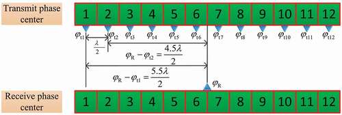
For the convenience of description, an array composed of 12 sub-arrays is taken as an example, as shown in Figure 1. Assume that each sub-array is used as a transmit sub-array, the phase centres of the transmit antenna are ${\phi }_{\mathrm{t}1},{\phi }_{\mathrm{t}2},\cdots ,{\phi }_{\mathrm{t}12}$, the distance between the antenna phase centres is $\lambda /2$, and all the channels receive returns at the same time. Because the varying of the receive phase centre of each channel between adjacent pulses is consistent with the varying of the receive phase centre of the whole array, for simplification, the whole array is used to receive the signal, and the phase centre of the receive antenna is ${\phi }_{\mathrm{R}}$. The equivalent phase centres of transmit and receive are approximately equal to the midpoint position between the transmit and receive phase centres. According to this principle, the equivalent phase centre of the first transmit sub-array corresponding to the first pulse is ${\phi }_{\mathrm{R}\mathrm{T}1}$, and the equivalent phase centre of the second transmit sub-array corresponding to each pulse is ${\phi }_{\mathrm{R}\mathrm{T}2}$, as shown in Equation (5)(5) ${\phi }_{\mathrm{R}\mathrm{T}1}=\frac{{\phi }_{\mathrm{R}}-{\phi }_{\mathrm{t}1}}{2}=\frac{5.5\lambda }{4},\hspace{0.17em}{\phi }_{\mathrm{R}\mathrm{T}2}=\frac{{\phi }_{\mathrm{R}}-{\phi }_{\mathrm{t}2}}{2}=\frac{4.5\lambda }{4}$(5) . The moving distance of the equivalent phase centre of two adjacent transmit sub-array is $\mathrm{\Delta }\phi$, as shown in Equation (6)(6) $\mathrm{\Delta }\phi ={\phi }_{\mathrm{R}\mathrm{T}2}-{\phi }_{\mathrm{R}\mathrm{T}1}=\frac{\lambda }{4}$(6) .

Figure 1. Schematic of transmit and receive phase centres.

(5) ${\phi }_{\mathrm{R}\mathrm{T}1}=\frac{{\phi }_{\mathrm{R}}-{\phi }_{\mathrm{t}1}}{2}=\frac{5.5\lambda }{4},\hspace{0.17em}{\phi }_{\mathrm{R}\mathrm{T}2}=\frac{{\phi }_{\mathrm{R}}-{\phi }_{\mathrm{t}2}}{2}=\frac{4.5\lambda }{4}$(5)

(6) $\mathrm{\Delta }\phi ={\phi }_{\mathrm{R}\mathrm{T}2}-{\phi }_{\mathrm{R}\mathrm{T}1}=\frac{\lambda }{4}$(6)

By setting the value of $PRI$ and the moving distance of the equivalent phase centre, the speed of emulating aircraft motion can be obtained, that is $v=\mathrm{\Delta }\phi /PRI$.

Furthermore, there are three features in the aircraft motion emulation. First, since the moving direction of the aircraft motion is always perpendicular to the direction of the transmit antenna, the emulate aircraft motion is equivalent to the airborne multichannel radar working in side-looking mode. Second, because the distance and time of the movement between pulses are the same, the speed of aircraft motion emulation is constant. Third, the speed of aircraft motion emulation is related to the moving distance of the adjacent transmit sub-arrays and PRI.

2.2. Derivation of model parameters

In the aircraft motion, it can be found that the distance between the phase centres of transmit and receive antenna corresponding to each pulse and the target is different, which is caused by the movement between pulses. The transmit and receive antenna patterns corresponding to each pulse will be inconsistent due to the array amplitude and phase error. The amplitude and reflectivity of sea clutter are random variables. In response to the above problems, the research on the sea clutter model of aircraft motion emulation will be carried out next.

2.2.1. Instantaneous slant range and antenna pattern of the transmit and receive

In order to distinguish the transmit sub-array from the receive sub-array, Figure 2 shows a Cartesian coordinate system as $O-xyz$, where $y$-axis denotes the platform motion direction and $z$-axis denotes perpendicular to the sea surface. In addition, $H$ denotes the height of radar, ${\theta }_{\mathrm{t}}$ and ${\phi }_{\mathrm{t}}$ denote the elevation angle and azimuth angle of the sea surface scattering point $A$ relative to the transmit sub-array, and ${\theta }_{\mathrm{r}}$ and ${\phi }_{\mathrm{r}}$ denote the elevation angle and azimuth angle of the sea surface scattering point $A$ relative to the receive sub-array, respectively. In order to clearly distinguish the position of transmit and receive array, the transmit array and receive array are placed separately and parallel (actually the transmit and receive are the same array). Taking the phase centre of the first sub-array as the reference phase centre, $l$ is the distance between the first transmit sub-array and the centre of the reference phase. In Figure 2, each transmit sub-array consists of 4 sub-arrays, it has $M$ transmit sub-arrays, each receive channel corresponds to a sub-array, and there are $N$ receive sub-arrays.

Figure 2. Geometric model of the instantaneous slant range.

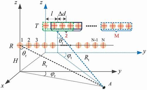
First, we derive the expression for the instantaneous slant range of transmit and receive. For simplicity, the aircraft motion emulation works in the one-column mode with one-column/PRI motion, that is the transmit sub-array containing one column and moves one column per PRI. Due to the spatial wave path difference, the instantaneous radial distance corresponding to the transmit sub-array and the receive sub-array changes with the coherent pulse varying. Then, the transmit distance $R_{\mathrm{t}}$ and receive distance $R_{\mathrm{r}}$ corresponding to the $n$th array element and $m$th pulse are shown in Equations (7)(7) $\begin{array}{c}{R}_{\mathrm{t}}=\sqrt{H^2+{(l+m\mathrm{\Delta }d+R_{0}sin\theta cos\phi )}^2+{\left(R_{0}sin\theta sin\phi \right)}^2}\\ \approx R_0+\frac{{(l+m\mathrm{\Delta }d)}^2}{2R_0}+(l+m\mathrm{\Delta }d)sin\theta cos\phi \end{array}$(7) and (8(8) $\begin{array}{c}{R}_{\mathrm{r}}=\sqrt{H^2+{(n\mathrm{\Delta }d+R_{0}sin\theta cos\phi )}^2+{\left(R_{0}sin\theta sin\phi \right)}^2}\\ \approx R_0+\frac{{(n\mathrm{\Delta }d)}^2}{2R_0}+n\mathrm{\Delta }dsin\theta cos\phi \end{array}$(8) ), in which power series expansion formulas are used, and higher-order terms are ignored.

(7) $\begin{array}{c}{R}_{\mathrm{t}}=\sqrt{H^2+{(l+m\mathrm{\Delta }d+R_{0}sin\theta cos\phi )}^2+{\left(R_{0}sin\theta sin\phi \right)}^2}\\ \approx R_0+\frac{{(l+m\mathrm{\Delta }d)}^2}{2R_0}+(l+m\mathrm{\Delta }d)sin\theta cos\phi \end{array}$(7)

(8) $\begin{array}{c}{R}_{\mathrm{r}}=\sqrt{H^2+{(n\mathrm{\Delta }d+R_{0}sin\theta cos\phi )}^2+{\left(R_{0}sin\theta sin\phi \right)}^2}\\ \approx R_0+\frac{{(n\mathrm{\Delta }d)}^2}{2R_0}+n\mathrm{\Delta }dsin\theta cos\phi \end{array}$(8)

where $R_0$ is the radial distance from the reference phase centre to the fixed scattering point $A$, the elevation angle and azimuth angle corresponding to the distance of the reference phase centre $\theta$ and $\phi$, and $\mathrm{\Delta }d$ is the distance between the two adjacent column sub-array.

Furthermore, because the transmit sub-array is always varying during the period of coherent pulse, the transmit sub-array antenna pattern is affected by the amplitude and phase error of each column. The multichannel radar antenna adopts plane array, which can be divided into an azimuth dimension linear array and an elevation dimension linear array. The azimuth dimension linear array is composed of $N$ sub-arrays, and the array pattern $f(\psi )$ is affected by the amplitude and phase error between channels. The elevation dimension linear array is composed of $K$ sub-arrays, and the array pattern $f(\theta )$ is affected by the amplitude and phase error between elements. Note that the smallest element antenna is dipole $f_{\mathrm{d}\mathrm{i}\mathrm{p}\mathrm{o}\mathrm{l}\mathrm{e}}(\theta ,\phi )$. Taking the above factors into consideration, the transmit and receive antenna patterns corresponding to each pulse are shown in Equations (9)(9) $f_{\mathrm{T}}\left(\theta ,\phi \right)=f_{\mathrm{d}\mathrm{i}\mathrm{p}\mathrm{o}\mathrm{l}\mathrm{e}}(\theta ,\phi )f(\psi )f(\theta )$(9) and (10(10) $f_{\mathrm{R}}\left(\theta ,\phi \right)=f_{\mathrm{d}\mathrm{i}\mathrm{p}\mathrm{o}\mathrm{l}\mathrm{e}}(\theta ,\phi )f(\theta )$(10) ), respectively.

(9) $f_{\mathrm{T}}\left(\theta ,\phi \right)=f_{\mathrm{d}\mathrm{i}\mathrm{p}\mathrm{o}\mathrm{l}\mathrm{e}}(\theta ,\phi )f(\psi )f(\theta )$(9)

(10) $f_{\mathrm{R}}\left(\theta ,\phi \right)=f_{\mathrm{d}\mathrm{i}\mathrm{p}\mathrm{o}\mathrm{l}\mathrm{e}}(\theta ,\phi )f(\theta )$(10)

where the dipole antenna is shown in (11), where in the backlobe region the pattern is scaled by the assumed backlobe level $b_{\mathrm{e}}$.

(11) $f_{\mathrm{d}\mathrm{i}\mathrm{p}\mathrm{o}\mathrm{l}\mathrm{e}}(\theta ,\phi )=\{\begin{array}{c}cos\phi -{90}^{\mathrm{o}}\le \phi \le {90}^o\\ b_{\mathrm{e}}cos\phi \hspace{0.17em}{90}^o\le \phi \le {270}^o\end{array}$(11)

The elevation dimensional linear array pattern is shown in (12), and the azimuth dimensional linear array pattern is shown in (13).

(12) $f(\theta )=\sum _{k=1}^K{E}_{\mathrm{r}\mathrm{\_}\mathrm{d}\mathrm{i}\mathrm{p}\mathrm{o}\mathrm{l}\mathrm{e}}\left(k\right)exp\left\{-j\frac{2\pi \mathrm{\Delta }d}{\lambda }\left(k-1\right)\left(cos\theta -cos{\theta }_0\right)\right\}$(12)

(13) $\begin{array}{c}f(\psi )=\sum _{n=1}^N{E}_{\mathrm{r}\mathrm{\_}\mathrm{a}\mathrm{r}\mathrm{r}\mathrm{a}\mathrm{y}}\left(n\right)exp\left\{-j\frac{2\pi \mathrm{\Delta }d}{\lambda }\left(n-1\right)\left(sin\theta cos\phi -sin{\theta }_{0}cos{\phi }_0\right)\right\}\\ =\sum _{n=1}^N{E}_{\mathrm{r}\mathrm{\_}\mathrm{a}\mathrm{r}\mathrm{r}\mathrm{a}\mathrm{y}}\left(n\right)exp\left\{-j\frac{2\pi \mathrm{\Delta }d}{\lambda }\left(n-1\right)\left(cos\psi -cos{\psi }_0\right)\right\}\end{array}$(13)

where $E_{\mathrm{r}\mathrm{\_}\mathrm{a}\mathrm{r}\mathrm{r}\mathrm{a}\mathrm{y}}\left(n\right)$ is the amplitude and phase error between channels, $E_{\mathrm{r}\mathrm{\_}\mathrm{d}\mathrm{i}\mathrm{p}\mathrm{o}\mathrm{l}\mathrm{e}}\left(k\right)$ is the amplitude and phase error between elements, $\psi$ is the space cone angle, and $\left({\theta }_0,{\phi }_0\right)$ is the direction of the antenna main lobe.

2.2.2. Sea clutter space-time signal model

The radar sea clutter from a dynamic sea surface is complex, and it depends on a variety of external factors such as ocean currents, wind speed, sea depth, as well as the radar waveform and viewing geometry. The sea surface radial velocity and the sea clutter reflectivity are the dynamic variables. Let ${\chi }_l(n,m)$ be the complex sample from the $n$th element, $m$th pulse, at the $l$th sample time (range gate). The $l$th isorange ring can be divided into $N_{\mathrm{c}}$ equally sized clutter patches, so the return is the integral of different clutter patches from different azimuth angles.

(14) ${\chi }_l(n,m)=\sum _{l=1}^{N_{\mathrm{c}}}\sqrt{{\xi }_l}y\left(\theta ,{\phi }_l\right)e^{j\vartheta \left(\theta ,{\phi }_l\right)}\otimes e^{j\varpi \left(\theta ,{\phi }_l\right)}$(14)

where $y\left(\theta ,{\phi }_l\right)$ is a random sequence satisfying a certain distribution; $\vartheta \left(\theta ,{\phi }_l\right)$ is the spatial frequency, shown in Equation (15)(15) $\vartheta \left(\theta ,{\phi }_l\right)=2\pi n\frac{\mathrm{\Delta }d}{\lambda }cos\theta cos{\phi }_l$(15) ; $\varpi \left(\theta ,{\phi }_l\right)$ is the normalized Doppler frequency, shown in Equation (16)(16) $\varpi \left(\theta ,{\phi }_l\right)=2\pi \left(m\frac{2V}{\lambda PRF}cos\theta cos{\phi }_l+\frac{2v_{\mathrm{s}\mathrm{e}\mathrm{a}}}{\lambda }\right)$(16) ; $\otimes$ is the Kronecker product; $V$ is the platform speed; and $v_{\mathrm{s}\mathrm{e}\mathrm{a}}$ is the sea surface radial velocity.

(15) $\vartheta \left(\theta ,{\phi }_l\right)=2\pi n\frac{\mathrm{\Delta }d}{\lambda }cos\theta cos{\phi }_l$(15)

(16) $\varpi \left(\theta ,{\phi }_l\right)=2\pi \left(m\frac{2V}{\lambda PRF}cos\theta cos{\phi }_l+\frac{2v_{\mathrm{s}\mathrm{e}\mathrm{a}}}{\lambda }\right)$(16)

where ${\xi }_l$ is clutter to noise ratio (CNR) corresponding to the ${\phi }_l$ azimuth of the $l$th clutter isorange ring.

(17) ${\xi }_l=\frac{P_{\mathrm{t}}{G}_{\mathrm{t}}\left(\theta ,{\phi }_l\right)g\left(\theta ,{\phi }_l\right){\lambda }^2{\sigma }_l}{{\left(4\pi \right)}^3{N}_0{L}_{\mathrm{s}}{R}_{\mathrm{t}}^2{R}_{\mathrm{r}}^2}$(17)

where $P_{\mathrm{t}}$ is the transmit power, $N_0$ is the noise power, $L_{\mathrm{s}}$ is the system losses, $G_{\mathrm{t}}\left(\theta ,{\phi }_l\right)$ is the sub-array transmit power gain of the ${\phi }_l$ azimuth, and $g\left(\theta ,{\phi }_l\right)$ is the receive element gain of the ${\phi }_l$ azimuth.

(18) $G_{\mathrm{t}}\left(\theta ,{\phi }_l\right)=G_{\mathrm{t}}{f}_{\mathrm{T}}\left(\theta ,{\phi }_l\right)$(18)

(19) $g\left(\theta ,{\phi }_l\right)=G_{\mathrm{r}}{f}_{\mathrm{R}}\left(\theta ,{\phi }_l\right)$(19)

where $G_{\mathrm{t}}$ is the transmit element gain and $G_{\mathrm{r}}$ is the receive element gain. The effective RCS of the azimuth ${\phi }_l$ is therefore

(20) ${\sigma }_l={\sigma }_{\mathrm{o}}\left(\theta ,{\phi }_l\right)R_{\mathrm{r}}\mathrm{\Delta }\phi \mathrm{\Delta }R$(20)

where ${\sigma }_{\mathrm{o}}\left(\theta ,{\phi }_l\right)$ is the area reflectivity of sea surface. Various models for the sea clutter reflectivity have been proposed. $\mathrm{\Delta }\phi =2\pi /N_{\mathrm{c}}$ is the minimum azimuth unit of division, and $\mathrm{\Delta }R$ is the radial distance resolution.

According to the above derivation, the space-time snapshot needs to be further processed to obtain the eigen spectra and power spectrum. Assume that the clutter is homogeneous, and the space-time snapshots corresponding to each range loop are independent and identically distributed. The maximum likelihood estimation principle is used to estimate the space-time covariance matrix (Capon, Greenfield and Kolker 1967).

(21) $\hat{R}=\frac{1}{L}\sum _{l=1}^L{\chi }_l{\chi }_l^{\mathrm{H}}$(21)

where $L$ is the number of range gate, and $\mathrm{H}$ denotes conjugate transpose. The value of $L$ satisfies RMB rules (Reed, Mallett and Brennan 1974). Through the covariance matrix, it can obtain the Capon spectrum, which directly reflects the optimal performance of clutter suppression (Capon 1969).

(22) $P\left(\vartheta ,\varpi \right)=\frac{1}{\mathbf{v}{{\left(\vartheta ,\varpi \right)}^{\mathrm{H}}}^{\hspace{0.17em}}{\stackrel{\mathbf{ˆ}}{\mathbf{R}}}^{-1}\mathbf{v}\left(\vartheta ,\varpi \right)}$(22)

where $\mathbf{v}\left(\vartheta ,\varpi \right)$ is the $NM\times 1$ dimension space-time steering vector; it can be obtained by the Kronecker of the time steering vector $\mathbf{b}(\varpi )$ and the space steering vector $\mathbf{a}\left(\vartheta \right)$.

(23) $\begin{array}{c}\mathbf{v}\left(\vartheta ,\varpi \right)=\mathbf{b}\left(\varpi \right)\otimes \mathbf{a}\left(\vartheta \right)\\ \mathbf{b}(\varpi )=\left[1;e^{j2\pi \varpi };\hspace{0.17em}\cdots ;e^{j(M-1)2\pi \varpi }\right]\\ \mathbf{a}\left(\vartheta \right)=\left[1;e^{j2\pi \vartheta };\cdots ;e^{j(N-1)2\pi \vartheta }\right]\end{array}$(23)

where $\varpi$ is the normalized Doppler frequency, $\vartheta$ is the normalized spatial frequency.

3. Results

Section 2 has established the sea clutter model of aircraft motion emulation, while this section will validate the model with simulated data and measured data. We will use the eigenvalue number and the clutter ridge spread width under different sea states to verify the model. Before the model validation, this paper proposes the calculation rule of eigenvalue number of sea clutter and spread width of sea clutter ridge.

Compared with land clutter eigen spectra, there is no obvious sharp cut-off in the sea clutter eigen spectra. The clutter subspace and the noise subspace are more difficult to distinguish. Note that clutter eigenvalue represents the clutter energy distribution. Therefore, the clutter subspace and the noise subspace can be distinguished with the CNR. If the eigenvalue is greater than the threshold using CNR, the number corresponding to this eigenvalue is the eigenvalue number. As shown in Figure 3(a), the sea clutter eigenvalue number is 52 with the CNR is 40 dB.

Figure 3. Calculation rule of the clutter eigenvalue number and the spread width of 3 dB clutter ridge.

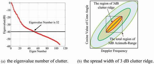
Due to the sea surface complicated movement, the sea clutter ridge of the power spectrum shows a great broadening phenomenon in the azimuth-Doppler plane, which is difficult to describe quantitatively. This paper proposes the clutter ridge spread width as a quantitative description of the sea clutter ridge broadening phenomenon. In order to describe the expansion of the space-time power spectrum, the definition of the spread width of the clutter ridge is given here. For simplicity, the clutter ridge corresponding to the 3 dB drop of the space-time power spectrum is referred to as the 3 dB clutter ridge, and the ideal clutter ridge width is the space-time power spectrum corresponding to the ideal condition. Then, the clutter ridge spread width is defined by the ratio of the 3 dB clutter ridge relative to the ideal clutter ridge width. As shown in Figure 3(b), when calculating the spread width of 3 dB clutter ridge, the following steps are used: first, find the maximum value corresponding to the power spectrum in the azimuth-Doppler plane. By holding the azimuth angle of maximum value fixed and varying the Doppler frequency, the Doppler spectrum corresponding to the azimuth angle of the maximum value can be obtained. Based on above Doppler spectrum, the width of the 3 dB clutter ridge can be obtained with the maximum value of the Doppler spectrum dropping by 3 dB, which is the black dashed line projected from the red ellipse to the Doppler domain in Figure 3(b). Second, because the working model of aircraft motion emulation is equivalent to the airborne radar in side-looking mode, the azimuth-Doppler plane area of 3 dB clutter ridge can be calculated by the width of 3 dB clutter ridge. If the spectrum width is $P$, the azimuth-Doppler plane area is $S=P^2$, which corresponding to the area of the black dashed box in Figure 3(b). Furthermore, the spread width of the ideal clutter ridge is 1, which can be known from its definition. Therefore, if the number of the resolution units corresponding to the 3 dB clutter ridge is $Q$, the spread width of the 3 dB clutter ridge is $Q/S$, which is the area of the orange ellipse inside the black dashed box, as shown in Figure 3(b).

Using the above calculation method, the eigenvalue number and the spread width of 3 dB clutter ridge can be described quantitatively. It is easy to know that the more the eigenvalue number and the wider the spread width of the 3 dB clutter ridge, the greater influence of sea surface motion on the space-time decorrelation.

3.1. Simulated data

From the sea clutter model of the aircraft motion emulation established in Section 2, it can be seen that the focus of the simulated data is the space-time snapshots. Once the space-time snapshot is known, the covariance matrix can be calculated by averaging the space-time snapshots, and then the eigenspectral and space-time power spectrum can be calculated by the covariance matrix. The space-time snapshot corresponding to each range gate is the sum of the space-time snapshot of multiple azimuth blocks. While the simulation of each azimuth block involves many parameters, such as the reflectivity of the sea clutter, amplitude statistical distribution model, CNR, transmit and receive antenna gain, etc. Following the steps in Figure 4, the simulated data of the emulating aircraft motion can be created.

Figure 4. Block diagram of simulation process of emulating aircraft motion sea clutter data.

The radar parameters of the simulated data to be set are as follows, L-band, VV polarization, the channel number is 12 and the pulse repetition frequency is 2000 Hz. The amplitude statistical distribution model of sea clutter adopts K distribution (Ward, Tough and Watts 2013); the shape parameters and scale parameters are determined by the sea states, which the sea states can be found in Table 1, and the sea states are classified by Douglas scale (Skolnik 2008). The wave height in Table 1 is the significant wave height (SWH) and the wind speed, which is classified by the Beaufort scale. When generating the simulated data, the value of SWH or wind speed under sea states 1–4 chooses the middle value of the SWH or wind speed in Table 1. At the same time, the spherically invariant random process method is used to simulate the clutter data satisfying the K distribution (Conte, Longo and Lops 1991), while the statistical model of the sea clutter reflectivity is the Morchin model (Xie, Yi and Kong 2015).

Table 1. Sea state descriptors (Douglas scale)

Sea state	1	2	3	4
Wind speed (ms ^> ^−1)	0 ~ 3.60	3.60 ~ 6.17	6.17 ~ 8.23	8.23 ~ 9.77
SWH (m)	0 ~ 0.3	0.3 ~ 0.91	0.91 ~ 1.52	1.52 ~ 2.44

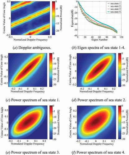
There are two kinds of aircraft motion emulation working mode under sea states 1–4. One is the one-column mode with two-column/PRI motion, the other is 4-column mode with one-column/PRI motion in the sea state 2. Figure 5(a) shows that the Doppler clutter ridge is folded over, which is consistent with the Section 2.1.1. Under sea states 1–4, 4-column mode with one-column/PRI motion has different eigenspectral, as shown in Figure 5(b). At the same eigenvalue threshold, it can be seen that the eigenvalue number corresponding to higher sea state is greater than the eigenvalue number corresponding to lower sea state. Figure 5(c-f), respectively, corresponds to the space-time power spectrum, which belongs to the 4-column mode with one-column/PRI motion. It is clearly found that the spread width of the sea clutter ridge corresponding to higher sea state is larger than the spread width of the sea clutter ridge corresponding to lower sea state.

Figure 5. Eigen spectra and power spectrum of simulated data.

3.2. Measured data

In this section, the effectiveness of the sea clutter model of aircraft motion is validated by the measured sea clutter data, which is measured by L-band shore-based multichannel radar in the central Yellow Sea of China. The radar parameters and the motion emulation working mode are consistent with the simulation parameters in Section 3.1.1. During the sea clutter measurement experiment, Datawell Waverider 4 provides the information of SWH, wave direction and cross-zero period with a data rate of a sample per 30 minutes, and Lufft WS700-UMB also measures real-time wind speed and wind direction with a data rate of a sample per 5 minutes. In order to compare the influence of sea state on the eigen spectra and space-time power spectrum. The sea state parameters corresponding to the real measured clutter data are shown in Table 2. It is need to be clearly stated that all the parameters in Table 2 are the average value.

Table 2. Sea state parameters of real measured clutter data

Sea state	SWH (m)	Wave direction (°)	Wave periods (s)	Wind speed (ms^−1)	Wind direction (°)
1	0.29	16,405	2.67	2.2	211.3
2	0.57	161.1	3.59	7.4	205.2
3	1.07	180.2	4.19	10.2	212.7
4	2.16	146.7	5.14	21.6	207.8

It should be noted that the real measured data are all processed by amplitude and phase correction. Also, what needs to be explained is that the data used in this paper comes from many sets of data with the same characteristics.

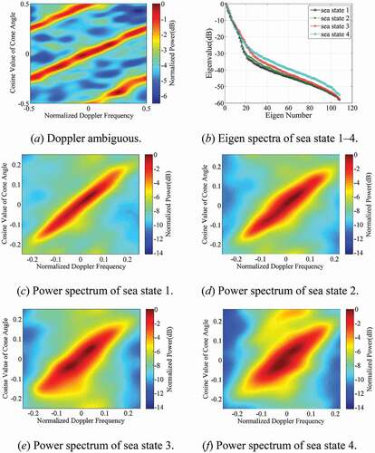
Similar to the simulation data, the one-column mode with two-column/PRI motion works in the sea state 2, which is equivalent to the shift of the phase centre of transmit sub-array is $\lambda /2$, so the power spectrum in Doppler domain is ambiguous, as shown in Figure 6(a). When the 4-column mode with one-column/PRI motion works in the sea states 1–4, the eigen spectra and space-time power spectrum are shown in Figure 6(b-f). In Figure 6(b)，with a certain eigenvalue threshold, the number of sea clutter eigenvalue increases as the sea state become higher. Just like the number of sea clutter eigenvalue change with sea states, it is found that the spread width of the space-time spectrum increases as the sea state become higher.

Figure 6. Eigen spectra and power spectrum of real measured data.

3.3. Comparison of the simulated data and measured data

The comparison of the real and simulated aircraft motion emulation sea clutter data in different sea states is demonstrated in Figures 5 and 6. With averaging 100 sets of measured data processing results under each sea state, the eigenvalue number of sea clutter and the spread width of 3 dB sea clutter ridge can be obtained, as shown in Table 3. The following comparison from three aspects are working mode, eigenvalue number, and spread width of 3 dB clutter ridge. First, comparing Figures 5(a) and 6(a), it is found that the space-time spectrum of the clutter is ambiguous. The reason for this phenomenon is that the distance of the phase centre of transmit sub-array moving per pulse repetition period is greater than half wavelength. Second, for the sea clutter eigenspectral, as shown in Table 3, if the threshold is 35 dB (CNR = 35 dB), the difference in eigenvalue number of the simulated data between the sea state 2 and sea state 4 is 15, while the difference in eigenvalue number of the measured data between sea state 2 and sea state 4 is 14. It is easy to know that the difference of eigenvalue number between simulated data and measured data is 1 under sea state 2 and 4. Also, the difference of eigenvalue number between simulated data and measured data is 5 under sea states 1 and 3. It can be seen that the difference of eigenvalue number is basically same under sea states 2 and 4 or sea states 1 and 3. Third, for the spectrum width of 3 dB clutter ridge, as shown in Table 3, the spread width of 3 dB clutter ridge corresponding to sea state 4 is almost twice that of sea state 2 in both simulated data and measured data, and it shows the same trend between sea states 1 and 3. Furthermore, as shown in Table 3, the eigenvalue number of simulated data is slightly greater than that of measured data, and the spread width of 3 dB clutter ridge shows the same result. It is clearly known that the eigenvalue number and the spread width of 3 dB clutter ridge of measured data are more than 79.5% of that belonging to simulated data. It is found that the simulated data and measured data show the same trend under the same sea state.

Table 3. Eigenvalue number and the spread width of 3 dB clutter ridge

Sea state	Eigenvalue number			Spread width of 3 dB clutter ridge
	Simulated data	Measured data	Percent (%)	Simulated data	Measured data	Percent (%)
1	30	26	86.7	3.5	2.9	82.3
2	39	31	79.5	4.8	4.3	89.6
3	45	36	80.0	7.3	6.2	84.9
4	54	45	83.3	9.8	8.5	86.7

From the comparison result, it shows that the sea clutter model of aircraft motion emulation established in Section 2 is valid. At the same time, it is found that the simulated data generated by the sea clutter model of aircraft motion emulation can better fit the measured data under sea states 1–4.

4. Discussion

Aircraft motion emulation can be implemented by shore-based multichannel radar, which is based on the IDPCA technique and the technique of transmit and receive antenna sharing the same array. Based on the implementation of aircraft motion emulation, this paper theoretically derives expression of the instantaneous distance and antenna pattern of the transmit and receive, then establishes sea clutter space-time signal model of aircraft motion emulation with the statistical model of amplitude distribution and sea clutter reflectivity. In order to verify the proposed theory, the simulated and real measured aircraft motion emulation data are compared in different sea states, and the results show that same change trend. It means that the shore-based multichannel radar can obtain sea clutter data with space-time coupling characteristics by working in the mode of aircraft motion emulation, which lays the foundation for the sea clutter measurement experiments of aircraft motion emulation. Additionally, in terms of the statistical model of sea clutter reflectivity and amplitude distribution, it can be further investigated in future work to obtain the model, which can reflect the statistical characteristics of real measured data.

Acknowledgements

The authors would like to express their sincere thanks to the members of the clutter research team in the China Research Institute of Radiowave Propagation for their work on sea clutter experiments.

Disclosure statement

No potential conflict of interest was reported by the author(s).

Additional information

Funding

This work was supported in part by National Natural Science Foundation of China under Grant [61801446 and U2006207].

References

- Aboutanios, E. and L. Rosenberg. 2019. “Multichannel Target Detection for Maritime Radar.” Paper presented at the 2019 53rd Asilomar Conference on Signals, Systems, and Computers, November 3-6. doi:https://doi.org/10.1109/IEEECONF44664.2019.9048948.
- Cai, Z., M. Zhang, J. Wang, J. Chen, and J. Zhao. 2016. “A Reassigned Bilinear Transformation and Gaussian Kernel Function-Based Approach for Detecting Weak Targets in Sea Clutter.” International Journal of Remote Sensing 37 (23): 5668–5686. doi:https://doi.org/10.1080/01431161.2016.1246774.
- Capon, J. 1969. “High Resolution Frequency Wavenumber Spectrum Analysis.” Paper Presented at the Proceedings of the IEEE 57 (8): 1408–1418. doi:https://doi.org/10.1109/PROC.1969.7278.
- Capon, J., R. J. Greenfield, and R. J. Kolker. 1967. “Multidimensional Maximum-Likelihood Processing of a Large Aperture Seismic Array.” Paper Presented at the Proceedings of the IEEE 55 (2): 192–211. doi:https://doi.org/10.1109/PROC.1967.5439.
- Conte, E., M. Longo, and M. Lops. 1991. “Modelling and Simulation of Non-Rayleigh Radar Clutter.” IEE Proceedings F Radar and Signal Processing 138 (2): 121–130. doi:https://doi.org/10.1049/ip-f-2.1991.0018.
- Gracheva, V. and D. Cerutti-Maori. 2012. “STAP Performance of Sea Clutter Suppression in Dependency of the Grazing Angle and Swell Direction for High Resolution Bandwidth.” Paper presented at the IET International Conference on Radar Systems, October 22-25. doi:https://doi.org/10.1049/cp.2012.1690.
- Gracheva, V. and D. Cerutti-Maori. 2013. “First Results of Maritime MTI with PAMIR Multichannel Data.” Paper presented at the 2013 International Conference on Radar, September 9-12. doi:https://doi.org/10.1109/RADAR.2013.6652032.
- Gracheva, V. and J. Ender. 2016. “Multichannel Analysis and Suppression of Sea Clutter for Airborne Microwave Radar Systems.” IEEE Transactions on Geoscience and Remote Sensing 54 (4): 2385–2399. doi:https://doi.org/10.1109/TGRS.2015.2500918.
- Guerci, J. R. 2015. Space-Time Adaptive Processing for Radar. 2nd ed. Boston: Artech House.
- Huang, P., Z. Zou, X. Xia, X. Liu, G. Liao, and Z. Xin. 2021. “Multichannel Sea Clutter Modeling for Spaceborne Early Warning Radar and Clutter Suppression Performance Analysis.” IEEE Transactions on Geoscience and Remote Sensing 59 (10): 8349–8366. doi:https://doi.org/10.1109/TGRS.2020.3039495.
- Kemkemian, S., J. Degurse, and L. Lupinski. 2015. “Performance Assessment of Multi-Channel Radars Using Simulated Sea Clutter.” Paper presented at the 2015 IEEE Radar Conference, May 10-15. doi:https://doi.org/10.1109/RADAR.2015.7131143.
- Klemm, R. 2006. Principles of Space-Time Adaptive Processing. 3rd ed. London: The Institution of Engineering and Technology.
- Li, X., P. Shui, X. Xia, J. Zhang, and X. Shi. 2020. “Analysis of UHF-Band Sea Clutter Reflectivity at Low Grazing Angles in Offshore Waters of the Yellow Sea.” International Journal of Remote Sensing 41 (19): 1–14. doi:https://doi.org/10.1080/01431161.2020.1760395.
- Machhour, S. and S. Kemkemian. 2021. “Improved Sea-Clutter Modelling for Multichannel Processing (STAP).” Paper presented at the 2021 21st International Radar Symposium (IRS), June 21-23. doi:https://doi.org/10.23919/IRS51887.2021.9466184.
- Majdolashrafi, P., M. Ardebilipour, and Y. Rajabzadeh. 2021. “Time-Dependent Diffusion Model for Sea Clutter Dynamics.” International Journal of Remote Sensing 42 (18): 6818–6836. doi:https://doi.org/10.1080/01431161.2021.1941387.
- McDonald, M. K. and D. Cerutti-Maori. 2016. “Coherent Radar Processing in Sea Clutter Environments, Part 1: Modelling and Partially Adaptive STAP Performance.” IEEE Transactions on Geoscience and Remote Sensing 52 (4): 1797–1817. doi:https://doi.org/10.1109/TAES.2016.140897.
- Melvin, W. 2004. “A STAP Overview.” IEEE Aerospace and Electronic Systems Magazine 19 (1): 9–35. doi:https://doi.org/10.1109/MAES.2004.1263229.
- Pan, X., G. Liao, and Z. Yang. 2019. “PolSar Ship Detection Based on the Contrast Enhancement of Polarimetric Scattering Differences.” International Journal of Remote Sensing 40 (18): 7071–7083. doi:https://doi.org/10.1080/01431161.2019.1601278.
- Reed, I. S., J. D. Mallett, and L. E. Brennan. 1974. “Rapid Convergence Rate in Adaptive Arrays.” IEEE Transactions on Aerospace and Electronic Systems 10 (6): 853–863. doi:https://doi.org/10.1109/TAES.1974.307893.
- Rosenberg, L. 2021. “Parametric Modeling of Sea Clutter Doppler Spectra.” IEEE Transactions on Geoscience and Remote Sensing. pp 1–9. doi:https://doi.org/10.1109/TGRS.2021.3107950.
- Shui, P. and Y. Shi. 2012. “Subband ANMF Detection of Moving Targets in Sea Clutter.” IEEE Transactions on Aerospace and Electronic Systems 48 (4): 3578–3593. doi:https://doi.org/10.1109/TAES.2012.6324742.
- Skolnik, M. I. 2008. Radar Handbook, 15.6. 3rd ed. New York: McGraw Hill.
- Suresh, B. N., J. A. Torres, and W. L. Melvin. 1996. “Processing and Evaluation of Multichannel Airborne Radar Measurements (MCARM) Measured Data.” Paper presented at the Proceedings of International Symposium on Phased Array Systems and Technology, October 15-18. doi:https://doi.org/10.1109/PAST.1996.566123.
- Titi, G. and D. F. Marshall. 1996. “The ARPA/NAVY Mountaintop Program: Adaptive Signal Processing for Airborne Early Warning Radar.” Paper presented at the 1996 IEEE International Conference on Acoustics, Speech, and Signal Processing Conference Proceedings, May 9-10. doi:https://doi.org/10.1109/ICASSP.1996.543572.
- Ward, J. 1994. Adaptive Processing for Airborne Radar. USA: Lincoln Laboratory. Tech. Rep, ESC-TR-94-109, 20-33.
- Ward, K., R. Tough, and S. Watts. 2013. Sea Clutter: Scattering, the K Distribution and Radar Performance. Vols. 75–87. 2nd ed. London: Institution of Engineering and Technology.
- Xie, M., W. Yi, and L. Kong. 2015. “Knowledge-Aided Space-Time Adaptive Processing Based on Morchin Model.” Paper presented at IET International Radar Conference 2015, October 14-16. doi:https://doi.org/10.1049/cp.2015.1268.
- Xin, Z., G. Liao, Z. Yang, Y. Zhang, and H. Dang. 2016. “A Deterministic Sea-Clutter Space-Time Model Based on Physical Sea Surface.” IEEE Transactions on Geoscience and Remote Sensing 54 (11): 659–6673. doi:https://doi.org/10.1109/TGRS.2016.2587739.
- Zhang, J., Y. Zhang, Q. Li, and J. Wu. 2018. “A Time-Varying Doppler Spectrum Model of Radar Sea Clutter Based on Different Scattering Mechanisms.” Acta Physica Sinica 67 (3): 034101. doi:https://doi.org/10.7498/aps.20171612.
- Zhang, J., Y. Zhang, X. Xu, Q. Li, and J. Wu. 2020. “Estimation of Sea Clutter Inherent Doppler Spectrum from Shipborne S-Band Radar Sea Echo.” Chinese Physics B 29 (6): 068402. doi:https://doi.org/10.1088/1674-1056/ab888a.