Dynamic regionalization of the Panama Bight, Eastern Tropical Pacific, using remote sensing data

ABSTRACT

This study establishes the dynamic biogeographic regions (DBGRs) of the Panama Bight (PB) based on remote-sensing reflectance (R_rs412 and R_rs488) of the MODIS-Aqua sensor and the sea-surface temperature (SST) and the concentration of chlorophyll a (Chl-a) derived from the same sensor. Monthly images with a spatial resolution of 4 km from the MODIS-Aqua sensor were used for July 2002–July 2020. To define the DBGR, the first standardized empirical orthogonal function (SEOF₁) was calculated. Due to the low spatial variability in the PB, the number of DBGRs found with the analysis of the SST and Chl-a was lower than that found in the analysis of the R_rs. Therefore, the DBGRs of the PB were delineated based only on the study of the R_rs. The PB was divided into 11 DBGRs belonging to two provinces: oceanic and coastal. Five of the DBGRs were coastal, the others oceanic, including a transition one. The coastal regions were characterized by the highest averages of Chl-a and high SST. On the other hand, the regions located northeast of the PB (Panama Gulf, PB-transition, and Choco) were characterized by an average SST greater than 28°C and an average Chl-a between 0.8 and 1.0 mg·m⁻³. The DBGRs located further west (west and PB-west) showed an average SST greater than 28°C and the lowest concentrations of Chl-a. The DBGRs PB-east and PB-central, presented average SSTs of 26.7–27.1°C and average Chl-a concentrations lower than 0.5 mg·m⁻³. The south Ecuador DBGR presented the lowest average SST (<25 °C) and average Chl-a of 0.50 mg·m⁻³. Our approach allowed us to generate a dynamic regionalization of the PB, which most of the year has small SST and Chl-a gradients, making this an alternative to the homogeneous areas generated from the thermohaline structure.

KEYWORDS:

• Dynamic regionalization
• Eastern Tropical Pacific
• remote sensing reflectance
• MODIS

1. Introduction

One of the most important issues managing natural resources is the determination of biogeographic regions (BGRs) (Santamaría-Del Ángel et al. 2011). Unlike in terrestrial environments, where a BGR can be defined through a particular biome, in marine environments, the delimitation is more complex because the medium is a fluid with a three-dimensional structure, and the pelagic ecosystem has intricate interactions between the biotic component and the abiotic environment. In marine environments, this type of classification has been mainly focused on the delimitation of representative ecological systems for the declaration of protected areas or marine zoning as a tool to improve resource management (Spalding et al. 2007). Early classifications were qualitative (e.g. Bleakley, Kelleher and Wells 1995; Olson and Dinerstein 2002) and were limited in their spatial coverage or methodological approach. Later ones were based on oceanographic factors, such as the delimitation made by Longhurst (2007), using an extensive global database of chlorophyll profiles and defined a division of two levels of biomes and biogeochemical provinces for the entire planet.

In marine environments, each BGR results from a particular combination of physical, chemical, and biological factors, and the variation in each of these factors can have different effects in each region. These characteristic features make biogeographic regionalization an essential tool for environmental modelling. Topics such as the carbon cycle, climate change, interaction with fisheries (IOCCG 2008, 2009a), management of marine resources, and climate variability can be addressed through the identification of BGRs either by the use of in situ data (direct approach) or by the use of data derived from remote sensors (indirect approach). Applying the direct method requires a database with adequate spatial and temporal coverage, which large monitoring programs can only achieve. For example, Millán-Núñez, Álvarez-Borrego and Trees (1997), using data from the California Cooperative Oceanic Fisheries Investigations program, identified six BGRs for the California Current system. However, the high cost of collecting samples in the ocean is a limitation that does not allow the areas to have robust oceanographic monitoring programs, so in these cases, an alternative for delineating BGRs is to use the indirect approach with satellite images as virtual maps to generate a database of the surface layer of the ocean (Santamaría del Ángel et al. 2011). A BGR can be determined by the association patterns produced by the temporal and spatial variation between geo-positioned locations or virtual stations. Different mathematical approaches can be taken to determine the association patterns between virtual stations. One of the most common is multivariate analysis. Using this approach, Santamaría-Del-Ángel, Álvarez-Borrego and Muller-Karger (1994) found 14 BGRs in the Gulf of California from a principal component analysis through weekly compositions derived from the Coastal Zone Colour Scanner sensor images at a spatial resolution of 4 km per pixel.

If the discontinuities in the physical environment are strong, the limits of the BGR will be less ambiguous. These discontinuities or boundaries of the BGR are generally located along thermal fronts and frontal systems (Longhurst 2007). However, these limits are not static and vary on different scales of time and space, reflecting the ocean’s dynamic nature. To delineate dynamic biogeographic regions (DBGRs), Gonzalez-Silvera et al. (2004, 2006) proposed a new approach based on a combination of images of chlorophyll a (Chl-a) (SeaWiFS sensor) and sea-surface temperature (SST) (AVHRR sensor). The proposal suggested that the numerical combination of these two variables, represented by the first standardized empirical orthogonal function (SEOF1), integrates the biological features of the area (defined by Chl-a) with the physical characteristics (SST) and thus describes the synchronous variation between regions.

In the Panama Bight (PB), the dynamic structure of the waters has been evaluated by tracking the evolution of the thermohaline characteristics at the horizontal level. Through the use of surface oceanographic data from the El Niño Regional Study (ERFEN, from its name in Spanish) (direct approach), the Pacific Pollution Control Center (CCCP, from its name in Spanish) divided the Colombian Pacific Basin (CPB) into seven homogeneous zones: one coastal zone and six oceanic zones (CCCP 2002). Based on this proposal of homogeneous zones, Málikov and Villegas (2005) constructed time series of the SST for each zone as a contribution to research on the incidence of natural and anthropogenic phenomena and the evolution and structure of oceanographic and climatological parameters of the region, and as a contribution to projects on this incidence in social and economic aspects. On the other side, Moreno, Villegas and Málikov (2008) using SST and sea-surface salinity (SSS) data, identified six water masses delimiting homogeneous regions in the CPB, although seven were identified during the month of March. Of these, two were coastal, one transitional, and the rest oceanic.

Although the PB has oceanographic information in situ (temperature and salinity), such as that collected by the General Maritime Directorate of Colombia (DIMAR, for its name in Spanish) for the CPB since 1970 (Dimar 2020), there is no continuous monitoring month by month with adequate temporal coverage that would give us the necessary information to delineate the BGRs of the PB. Therefore, it is necessary to apply the indirect approach using data derived from remote sensors. For oceanographers who work with the optical properties of water, the issue of identifying water masses on the ocean surface can be resolved through a classification based on their optical properties because the optical predictors can provide additional dimensions of discrimination beyond those provided by traditional analyses of temperature and salinity (Oliver et al. 2004). Studies that use the optical properties of water provide fundamental information about the processes in the upper oceanic layer and can also be useful to improve the precision with which satellite data are interpreted, as in the case of continental waters with high amounts of coloured dissolved organic matter (CDOM) (Hochman, Muller-Karger and Walsh 1994). In addition, approaches based on Chl-a and SST in areas with little variability have not yielded robust results to define regions or their dynamic boundaries (Callejas-Jiménez et al. 2012). Therefore, an alternative to identify DBGRs is to use the normalized water-leaving radiance (nLw) or remote-sensing reflectance (R_rs) (Martin-Traykovski and Sosik 2003; Oliver et al. 2004; Santamaría-Del Ángel et al. 2011; Callejas-Jiménez et al. 2012; González-Minaya and Santamaría Del Ángel 2014). nLw and R_rs are optical parameters that describe the oceanic carbon cycle (IOCCG 2008). They are related to several components of the biogeochemical cycles and are associated with specific processes, giving us another way of studying the interactions between organisms and their environments (IOCCG 2009a).

Thus, this work aims to identify and delimit the DBGRs of the PB by an indirect approach using R_rs derived from images of the MODIS-Aqua sensor (R_rs 412 nm and R_rs 488 nm) and through a mathematical approach based on SEOF. This approach to delimiting DBGRs is an alternative to the classical approach that uses variables such as temperature and salinity. We believe that using the optical properties of water, such as R_rs, will provide a more significant amount of information and improve the discrimination of the homogeneous zones of the PB that have been delineated thus far with in situ data. This regionalization can be used to optimize oceanographic monitoring and manage the resources in the PB.

2. Data and methods

2.1. Study area

The Panama Bight (PB) was initially defined by Wooster (1959) as part of the Eastern Tropical Pacific (ETP) that extends between the Isthmus of Panama and Punta Santa Elena (2° S) in Ecuador, up to 81° W. Biogeographically, the region is more extensive, and is considered a coastal marine ecoregion of the ETP that includes waters of Panama, Colombia, Ecuador, and a portion of Costa Rica and extends to 84°45′ W (Spalding et al. 2007) (Figure 1).

Figure 1. Study area in the Panama Bight (pb).

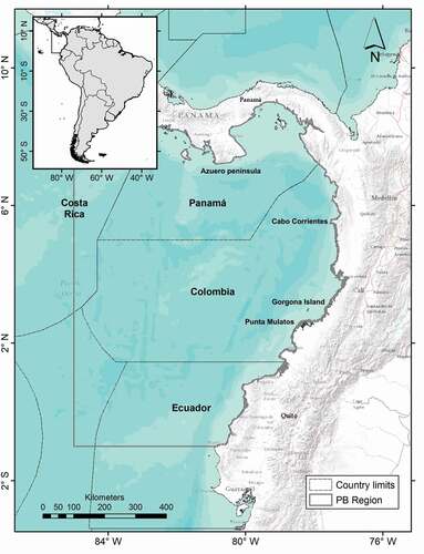
The PB is an area of great interest because it marks the eastern limit of the waters of the Equatorial Counter Current and because it presents a substantial interannual variability associated with El Niño South Oscillation (ENSO) (Fiedler and Talley 2006). Due to its position in a low-pressure equatorial concavity, the PB is strongly influenced by the ITCZ since the latter modulates the annual cycle of oceanographic and hydro climatological conditions (Wooster 1959; Wyrtki 1966; Forsbergh 1969; CCCP 2002; Poveda 2004) and generates mesoscale processes that in turn directly influence the climatology of the PB, such as the Panama jet (Chelton, Freilich and Esbensen 2000; Amador et al. 2006) and the Chocó jet (Poveda and Mesa 2000). The first of these processes occur during the end and beginning of the year (boreal winter) when the northeast trade winds pass through a low-lying area in the Isthmus of Panama, and jet streams (Panama jet) rapidly push the ITCZ to the south. As a result of this process, a seasonal upwelling event occurs between December and March in the Gulf of Panama and the central portion of the PB, which generates a decrease in SST and an increase in chlorophyll-a concentration (Chl-a) (Legeckis 1986; Badan-Dangon and Robinson 1998; Rodríguez-Rubio and Stuardo 2002; Corredor-Acosta et al. 2020).

The major currents that influence the ETP and, directly and indirectly, the PB are the equatorial system (North Equatorial Current, North Equatorial Counter Current, and South Equatorial Current) and the Peruvian Current. The South and North Equatorial Currents are driven by the northeast and southeast trade winds that blow towards the equator from the east, alternating their predominance throughout the year. When southeast trade winds predominate, the North Equatorial Current is located at approximately 10° N, and the South Equatorial Current is located at the geographical equator. Meanwhile, the North Equatorial Counter Current flows east through the ITCZ, where trade winds do not oppose it, so it is confined between 4° and 10° N (Wyrtki 1966). During March–April, the ITCZ is in its southernmost position, close to the geographical equator. The turn in the north Pacific intensifies, weakening the North Equatorial Counter Current, which at that time of the year is located west of the Galapagos Islands. During September–October, the situation is reversed: the ITCZ is north of 10° N, and the North Equatorial Counter Current strengthens and extends to the west of the PB (Badan-Dangon and Robinson 1998; Kessler 2006).

2.2. Dataset

Remote-sensing reflectance (R_rs) is a primary product produced by different space agencies. R_rs is an apparent optical property defined as R_rs = L_w/E_s, where L_w is the upward water-leaving radiance (Wm⁻²·sr⁻¹) and E_s is the descending irradiance at sea level (Wm⁻²). Therefore, the units of R_rs are sr⁻¹ (Mueller et al. 2003). The relationship of R_rs with the normalized radiance (nLw) is given by the relationship R_rs = nLw/F_o, where F_o is a constant of the solar irradiance in the upper part of the atmosphere (Valente et al. 2016). For the wavelength 412 nm, F_o = 171.183655 and for the wavelength 488 nm, F_o = 194.179092 (Thuillier et al. 2003). To generate the standard products of ocean colour, the Ocean Biology Processing Group of NASA uses bands 8–16 with central wavelengths from 412 nm to 870 nm of the moderate-resolution imaging spectroradiometer sensor found onboard the Aqua spacecraft (MODIS-Aqua). Thus, the primary products of ocean colour are the normalized water-leaving radiances (nLw) and R_rs from bands 8 to 14 (412 nm, 442 nm, 488 nm, 531 nm, 547 nm, 667 nm and 678 nm), while bands 15 and 16 (748 nm and 869 nm) are used to determine the type and optical thickness of aerosols for atmospheric correction (Franz et al. 2005). Because R_rs can be calibrated with greater precision than nLw, its use is recommended over nLw (Gordon and Voss 2004).

The R_rs of the MODIS-Aqua sensor images were obtained at wavelengths of 412 nm (R_rs412) (band 8) and 488 nm (R_rs488) (band 10). R_rs412 and R_rs488 are indicators of particulate organic carbon. Wavelength 412 is an indicator of CDOM and is therefore associated with a coastal influence, while wavelength 488 is sensitive to phytoplankton pigments (Morel and And 2009) and is less absorption by water components, making it an indicator of oceanic influence (IOCCG 2006). The images used were global, with an L3 processing level, with a monthly temporal resolution, and with a spatial resolution of 4 km. The time period considered was July 2002–July 2020 (19 years). In addition, SST and Chl-a (mg·m-3) images were obtained with the same level of processing and with the same spatial and temporal resolutions. The SST images were obtained only during the day, and those from the longwave infrared thermal bands at 11_µm and 12_µm (bands 31 and 32) were used. This dataset is distributed by the Physical Oceanography Distributed Active Archive Center (https://podaac.jpl.nasa.gov). The R_rs and Chl-a images were obtained from the ‘Ocean Colour web’ (http://oceancolor.gsfc.nasa.gov/) of the Ocean Biology Processing Group at NASA’s Goddard Space Flight Center.

2.3. Data analysis

The values associated with each pixel of each image (R_rs412, R_rs488, SST, and Chl-a), corresponding to the PB, were extracted using a routine in ArcGIS 10.5. Matrices of 36,086 pixels × 215 months for each product were constructed, which were the inputs into a SEOF analysis. From each matrix, the pixels of land and clouds were eliminated. The pixels that presented a percentage of missing data greater than 20% in the 2002–2020 series were eliminated from the matrix and then filled with the climatological average. The remaining missing data were spatially interpolated in ArcGIS 10.5 using the nearest neighbour routine even after filling in the data. The SEOF analysis yields the best numerical combination of the variables (in this case R_rs412-R_rs488, SST, and Chl-a) and captures the spatial and temporal variability (Santamaría-Del Ángel et al. 2011). The analysis distributes the total variance in a set of new data combined with original variables through a series of orthogonal patterns so that the first component explains the greater part of the variability of the data (Emery and Thompson 2014). Three SEOF analyses were performed: the first included R_rs412 and R_rs488, and the other two were for SST and Chl-a, respectively. In each case, the analysis was performed for the average year using the complete time series (2002–2020) and for the annual climatology (annual cycle of 12 months). In total, 39 SEOF analyses were performed using the R software packages ‘FactoMineR’ and ‘Factoextra’ (Kassambara 2017). The first component, or orthogonal empirical function, representing the best linear combination of the original variables, was standardized in terms of its standard deviation to facilitate its interpretation (SEOF₁), following the methods of Santamaría-Del Ángel et al. (2011) to identify DBGRs. The first component was interpolated in ArcGIS 10.5, and the contours of the standard deviations of SEOF₁ (±3) allowed us to identify the limits of the DBGRs. In interpreting SEOF₁, a value of 0 includes all the polynomial components that operate on its average value.

3. Results

The first component (PC1) for three SEOF analysis (R_rs412-R_rs488, SST and Chl-a) for the average year using the complete time series (2002–2020) and for the annual climatology had a contribution to the total variance ranged from 67 to 87%, while the contribution to the variance of PC2 was very low (between 3 and 7%). According to the regionalization found with the annual average R_rs412 - R_rs488 (Figure 2) from the SEOF analysis (PC1), the PB presented two provinces (oceanic and coastal) and eleven DBGRs (Table 1). The provinces were defined according the shelf continental (200 m isobath). The DBGRs that were on the continental shelf or part of them, were included in the coastal province and the rest in the oceanic province. The oceanic province introduced six DBGRs, including one transition, and the coastal province presented five DBGRs. The 11 DBGRs were R1) west: delimited between 2 and 3 standard deviations, and the smallest of the regions; R2) PB-west: delimited between 1 and 2 standard deviations; R3) PB-central: delimited between 0 and 1 standard deviation; R4) PB-east: delimited between −1 and 0 standard deviations; R5) South Ecuador, delimited between −2 and −1 standard deviations; R6) PB-transition, located between coastal and oceanic waters; R7) Panama Gulf; R8) Choco, delimited between −2 and −3 standard deviations; R9) coast-south, which included the coast of Ecuador and the Tumaco Bight in Colombia; R10) coast-north, which included the coastal waters of the Gulf of Panama and the east of the Azuero Peninsula; R11) coast-central, which included the coastal waters of Colombia between Gorgona island and ‘Cabo Corrientes’. All coastal regions showed deviations lower than −3 (Figure 2, Table 1).

Figure 2. Dynamic biogeographic regions (DBGRs) of the Panama Bight, generated from an analysis of the Orthogonal Empirical Function of the R_rs412 and R_rs488 remote-sensing reflectance of the MODIS-Aqua sensor (2002–2019). The left panel shows the first standardized empirical orthogonal Function (SEOF1) for the average annual, and the right panel shows the DBGRs. (R1) West; (R2) Panama Bight West; (R3) Panama Bight Central; (R4) Panama Bight East; (R5) South-Ecuador; (R6) Panama Bight Transition; (R7) Panama Gulf; (R8) Norte-Choco Region; (R9) Coast-South; (R10) Coast-North; and (R11) Coast-Central).

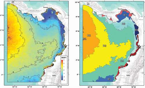
Table 1. Provinces and dynamic biogeographic regions (DBGR) of the Panama Bight (PB).

Province	DBGR		Standard deviation
Oceanic	R1	West	2;3
	R2	PB West	1;2
	R3	PB Central	0;1
	R4	PB East	−1;0
	R5	South-Ecuador	−2;-1
	R6	PB Transition	−2;-1
	R7	Panama Gulf	−3;-2
	R8	Chocó	−3;-2
Coastal	R9	Coast-South	<-3
	R10	Coast-North	<-3
	R11	Coast-Central	<-3

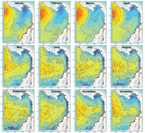
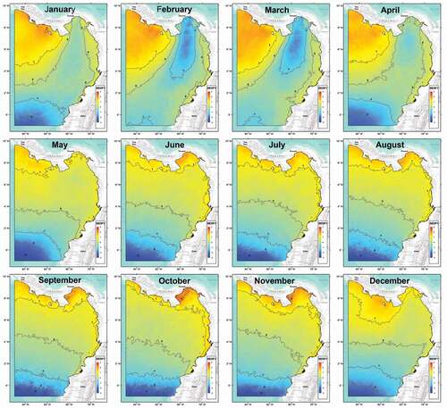
During the first quarter, the regionalization pattern was different from that in the rest of the year. R1 (west) area expanded towards the northeast of the PB and was largest during February. R2 (PB-west) contracted, and much of the PB was dominated by R3, R4, and R6 (PB-central, PB-east and PB-transition), while R5 (south Ecuador) disappeared. As of May, the configuration of the DBGRs was similar to that of the average year, although R5 remained absent, and the typical characteristics of the central region of the PB (standard deviations of 0–1) extended to a large part of the PB (Figure 3).

Figure 3. Climatology of the first standardized empirical orthogonal function (SEOF1), generated from the remote-sensing reflectance R_rs412 y R_rs488 of the MODIS-Aqua sensor (2002–2019).

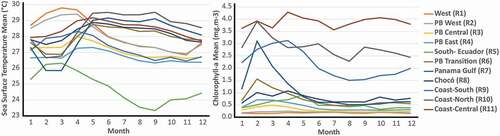
Considering the average year (Figure 2), the northern, central, and southern coastal DBGRs were characterized by the highest averages of Chl-a (>2.0 mg·m⁻³) and high SST values (>27.2 °C). On the other hand, the Panama Gulf, PB-transition and Choco regions, located northeast of the PB, were characterized by an average SST greater than 28°C and an average Chl-a between 0.8 and 1.0 mg·m⁻³. The DBGRs west and PB-west showed average SSTs greater than 28°C and the lowest concentrations of Chl-a (<0.20 mg·m⁻³). PB-east and PB-central, which occupied large parts of the PB, presented average SSTs between 26.7 and 27.1°C, and average Chl-a concentrations lower than 0.5 mg·m⁻³. Finally, the south Ecuador DBGR showed the lowest average SST (<25 °C) and average Chl-a values of 0.50 mg·m⁻³ (Figure 4).

Figure 4. Average of Sea Surface Temperature (SST) and Chlorophyll-a (Chl-a) of the dynamic biogeographic regions (DBGR) of the Panama Bight (PB).

Figure 5 shows the climatology of the SST and Chl-a of the 11 DBGRs of the PB found in the analysis. Besides the west and PB-west regions, which presentedsimilar average SST and Chl-a throughout the year, all the DBGRs had a characteristic signal and behaviour in these two variables (Figure 4). The regions located in the centre of the PB (R3, R4 and R6) and the coastal regions (R7, R8, R10, and R11) were strongly influenced by the Panama wind jet, and during the first quarter of the year, their SST decreased and Chl-a increased. In contrast, the coast-south, south Ecuador, west, and PB-west DBGRs showed a decrease in SST during the last quarter of the year, which was associated with strengthening the South Equatorial Current.

Figure 5. Average annual cycle of Sea Surface Temperature (SST) and Chlorophyll-a (Chl-a) of the dynamic biogeographic regions (DBGR) of the Panama Bight (PB) generated from an analysis of Orthogonal Empirical Function.

According to Callejas-Jiménez et al. (2012), the ratio R_rs412/R_rs488 can be used to differentiate coastal waters from ocean waters. Values >1 correspond to oceanic DBGRs, and values <1 correspond to coastal DBGRs. Figure 6 presents this relationship and denotes a separation between the two provinces. However, in the coastal province, it was observed that the coast-south, coast-central, and coast-north DBGRs had average values lower than 0.80, while Choco and Panama Gulf had values higher than 0.90. These two DBGRs, despite being limited by the coastal edge, presented optical characteristics closer to those of the oceanic province than the coastal province. Among the DBGRs of the oceanic province with an R_rs412/R_rs488 ratio >1, PB-transition presented the lowest average (1.07), so this DBGR presented optical characteristics of a mixed zone of oceanic and coastal waters. On the other hand, PB-west and west presented averages greater than 1.55, making them the regions with the most oceanic waters of the PB as defined by these optical descriptors.

Figure 6. Average of the R_rs412/R_rs488 ratio of the dynamic biogeographic regions (DBGR) of the Panama Bight (PB).

The regionalization performed for the SST (annual average) allowed us to find six main homogeneous regions (DBGRs) arranged latitudinally (Figure 7). From north to south, these were 1) north of the PB, located on the borders with Panama and Costa Rica and with standard deviations >1. 2) The central coastal zone of Colombia, located between southern ‘Cabo Corrientes’ and ‘Punta Mulatos’, with standard deviations >1. 3) The north-central region of the PB: delimited between 0 and 1 standard deviation. 4) South central region: delimited between 0 and −1 standard deviation. 4) Gulf of Panama: delimited between −1 and −2 standard deviations. 5) South transition, with standard deviations between −1 and −2. 6) South of the PB, with standard deviations <-2. The annual cycle of regionalization for SST (Figure 8) showed that during the first four months, the pattern found in the analysis of the average year changed considerably, as happened in the study of the R_rs. During these months, the entire central southwest–northeast axis was dominated by values that operated below the average (standard deviation equal to 0). However, from May on, with the onset of the predominance of southerly winds, there are changes in the regions, and their configuration was similar to that of the average year.

Figure 7. First standardized empirical orthogonal Function (SEOF1) for the average annual, generated from an analysis of the Orthogonal Empirical Function of Sea Surface Temperature (SST) (left panel) and surface Chlorophyll-a (Chl-a) (right panel), of the MODIS-Aqua sensor, time period 2002–2020.

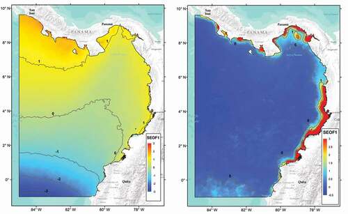
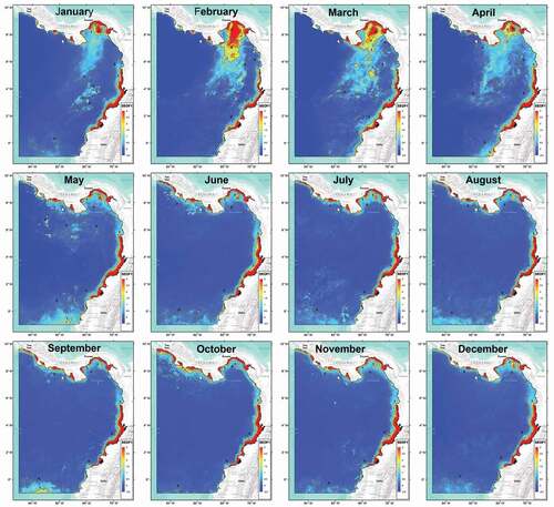
Figure 8. Climatology of the first standardized empirical orthogonal function (SEOF1), generated from the Sea Surface Temperature (SST) of the MODIS-Aqua sensor (2002–2019).

The regionalization analysis for Chl-a did not discriminate between DBGRs but allowed us to identify two provinces: the oceanic province with deviations <0 and the coastal province with deviations >1. There was also a southern zone of the PB that presented deviations >0 (Figure 7). In the first quarter, the Gulf of Panama and the area of influence that extends to the central part of the PB showed an increase in productivity, and standard deviations >1 were observed. May was a transition month in which the DBGRs were reconfigured, after which the structure of the average year was maintained between June and December (Figure 9).

Figure 9. Climatology of the first standardized empirical orthogonal function (SEOF1), generated from the Chlorophyll-a (Chl-a) of the MODIS-Aqua sensor (2002–2019).

4. Discussion

The analysis of DBGRs and their water masses is an active field of research due to its usefulness for describing processes such as ocean circulation, estimating the impact of river plumes, and identifying fronts and boundaries between water masses, which are important areas of mixing and biological activity, and to understand biogeochemistry at the basin scale (Martin-Traykovski and Sosik 2003; Oliver et al. 2004). Together, the results can also be helpful as a tool to improve resource management (Spalding et al. 2007). The classic approach to delimit dynamic homogeneous regions or DBGRs has been to use variables such as temperature and salinity, mainly through temperature-salinity diagrams, which are based on the conservative properties of water masses (Helland-Hansen 1916), and more recently through data derived from remote sensors (Gonzalez-Silvera et al. 2004; Gonzalez-Silvera, Santamaría-Del-Ángel and Millán-Núñez 2006). However, optical water predictors, such as remote-sensing reflectance (R_rs) or normalized water-leaving radiances (nLw), provide additional information that allows for better discrimination than analyses based on temperature and salinity.

Martin-Traykovski and Sosik (2003) presented a scheme to classify biogeochemical provinces based on the analysis of Chl-a and nLw at 420–443, 510–520 and 550–555 nm, which were selected as representative of different optical types of water and showed, for a region of the north-western Atlantic, that regions can be discriminated using the optical properties of water. Thus, DBGR classification based on nLw allowed us to understand the oceanic processes of the upper layer and contributed to improving the theoretical basis for implementing classification techniques based on time series of the optical properties of water and thus to monitor the types of water through seasonal and interannual changes. On the other hand, Oliver et al. (2004), in addition to using temperature data from the AVHRR sensor, used the R_rs measured at 490 nm (R_rs490) and 555 nm (R_rs555) to define regions over areas of the continental shelf of the mid-Atlantic.

For PB, the identification of homogeneous regions has been based on the study of the thermohaline characteristics of the surface layer. The regionalization carried out by CCCP (2002) for the CPB identified seven homogeneous zones: one coastal zone and six oceanic zones. The coastal zone was characterized by very high temperature and salinity oscillations due to the influence of the contributions of rivers and by heat flows and horizontal and vertical movements. A mixing zone could be identified (areas II and III), while oceanic waters represented zones IV–VII, and each zone presented particular characteristics of temperature, salinity, and density. Moreno, Villegas and Málikov (2008), using SST and SSS data, identified six water masses delimiting homogeneous regions in the CPB, which increased to seven during the month of March with the presence of the Panama jet. These regions were included in three large zones: a coastal zone, a mixed zone and an oceanic zone. Oscillations of SST and SSS generated the coastal zone due to freshwater from rivers, their heat flows, and vertical and horizontal movements. Water masses characterized the mixing zone with both coastal and oceanic SST and SSS values. The oceanic zone consisted of water masses with lower SST values than the coastal and mixed zones and higher SSS values than those of the other two zones.

The use of ocean colour data derived from remote sensors in the PB has been based on the study of the distribution of pigments (Chl-a) (Rodríguez-Rubio and Stuardo 2002; Corredor-Acosta et al. 2020). However, much of the coastal zone of the PB, mainly associated with Colombia and Ecuador, has basins with high rates of precipitation and high humidity, drainage with high volumes of water, and a high sediment load (Restrepo and López 2008), which make the waters on the continental shelf optically complex. In coastal environments with high levels of CDOM, the concentration of Chl-a derived from remote sensors can be overestimated, so the application of these algorithms to this type of water is not very useful. Furthermore, the quality of the information in these environments is often too low because atmospheric correction often fails for absorbent aerosols because standard atmospheric models cannot be applied (Gordon 1997) since the turbidity of coastal water violates the assumption of the absence of seawater radiation at near-infrared wavelengths (Siegel et al. 2000). Another challenge is that the algorithm to derive Chl-a often fails in waters with dissolved and suspended coloured materials without algae (O’Reilly and Werdell 2019).

Potential errors in obtaining the concentrations of the pigments can be avoided if the specific types of waters associated with the DBGR are identified and if the appropriate algorithms and corrections are applied. Thus, using classification techniques to identify the different types of water through the optical properties of ocean colour derived from remote sensing (R_rs and nLw) helps minimize the problems associated with the quantification of chlorophyll in coastal environments (Martin-Traykovski and Sosik 2003). However, no efforts have been made in the PB to identify mesoscale characteristics related to the limits of the types of water associated with the DBGR using this type of data (R_rs or nLw). Given the potential value of the information associated with ocean colour images because not only can we obtain the concentration of Chl-a, but we can also obtain values such as inherent optical properties, photosynthetic active radiation, particulate organic carbon, and R_rs, among others, and because it is possible to discern subtle differences between the types of waters of the DBGRs through the exploration of water optics, this study opted to use R_rs as a methodological approach to identify DBGRs of the PB. Additional analysis was also performed on SST and Chl-a to corroborate that the low variability across the PB, mainly during the second semester of the year, does not allow for adequate regionalization using this type of variable.

Similar to this study the use of R_rs412 and R_rs488 of the MODIS-Aqua sensor have also been used to define DBGRs on the island of Santo Domingo (González-Minaya and Santamaría Del Ángel 2014), in the Gulf of Mexico (Callejas-Jiménez et al. 2012), and in the Grand Caribe (Cañón 2010), showing that it performs well at regionalization where the variability is low or there is no significant gradient (Callejas-Jiménez et al. 2012). R_rs412 represents the CDOM absorption signal associated with the coast (Morel 1980; Mobley 1994; Morel and And 2009). Also known as the violet band, it is the brightest band (with the most dominant magnitude) in reflectance obtained by passive remote sensors that measure the colour of the ocean in waters with a chlorophyll concentration lower than 0.1 mg·m⁻³. This band has been used in two new families of OC algorithms (the OC5 and OC6 algorithms). According to O’Reilly and Werdell (2019), while the peak in the absorption of specific chlorophyll coincides with the 443-nm band present in most ocean colour sensors, the magnitude of the absorption of chlorophyll specifically at 412 nm can reach up to 70% of that obtained at 443 nm. Therefore, the inclusion of wavelengths shorter than 412 nm allows a better differentiation of the CDOM with respect to Chl-a, since these wavelengths are farther from the absorption peak of Chl-a and closer to the region of stronger absorption of CDOM. Therefore, several of the recently launched and planned ocean colour sensors (will) have bands with wavelengths less than 412 nm, such as PACE, Sentinel OLCI, and SGLI (O’Reilly and Werdell 2019).

On the other hand, wavelength 488 (R_rs488) is sensitive to phytoplankton pigments and can be associated with the oceanic zone (Morel and And 2009). This band has been used in some algorithms as the green part of the blue/green ratio when the chlorophyll content is high (O’Reilly et al. 1998). The algorithms used are typically based on the relations or radios of nLw or the R_rs in the visible light spectrum. The most commonly used ratio for MODIS-Aqua is L_w443/L_w550 or R_rs488/R_rs547 (Yang et al. 2018), while for SeaWiFS, it is R_rs490/R_rs555 (Cañón 2010). SeaWiFS band 490 is homologous to MODIS band 488.

We did not use the relationship between bands but rather their linear combination through the first orthogonal empirical function (SEOF₁), following the same logic as in the relationships between bands of the algorithms that study the colour of the ocean. According to IOCCG (2009b), the determination of dynamic regions can be based on SEOF since it is a powerful tool that quantifies the spatiotemporal variation of an area. SEOF1 was used because it explains most of the variability and the definition of limits between DBGRs. The numerical value of 0 of SEOF1 involves all the polynomial components that operate on its mean value, which allowed us to differentiate the coastal influence from the oceanic influence. In this study, SEOF1 was delimited by a standard deviation interval of −3 to +3. Santamaría-Del Ángel et al. (2011) described that the maximum values of the standard deviation of SEOF1 fluctuate between ±3.4 and ±4 in areas with low variability; when that variability increases, the values of SEOF₁ can be reduced to ± 1 to ±2. These authors used the same variables as in this study in an area characterized by strong gradients (Southern California Current System), observing SEOF1 values between ±1 and ±2. In other areas with strong variability in SST and Chl-a, such as the Brazil–Falkland Current and the delta of the Río de la Plata (Gonzalez-Silvera, Santamaría-Del-Ángel and Millán-Núñez 2006) and the Canal de Ballenas within the Gulf of California (Flores-de-Santiago et al. 2007), the standard deviation interval was approximately ±1. The range of SEOF1 is specific to each location, and the number of standard deviations depends on the variability in each site, showing a narrow range in areas with a strong gradient but increasing in areas with a weak gradient, as is the case of the PB where the delineation of DBGRs could be done with an interval of ±3. This confirms that the PB is an area with lower spatial variability than other areas and allows us to understand the results obtained with the regionalization using Chl-a and SST, which did not show a significant number of DGBRs.

Due to the low variability in PB, the number of DBGRs found in the SST and Chl-a analyses was lower than that found in the R_rs analysis. Therefore, the delineation of DBGRs of the PB was based only on the analysis of the R_rs. Two provinces were identified (oceanic and coastal), and a total of 11 DBGRs were identified. The provinces were defined according the shelf continental (200 m isobath). The DBGRs that were on the continental shelf or part of them, were included in the coastal province and the rest in the oceanic province. Five of the DBGR were coastal and six oceanic, including a transitional one. Among the coastal regions, coast-south (R9), coast-north (R10) and coast-central (R11) were different from Choco (R8) and Panama Gulf (R7). These regions, mainly those associated with the central–south coast of Colombia and the coast of Ecuador, are characterized by a strong continental influence due to the contribution of rivers, which affects the dynamics of nutrients and water turbidity (Restrepo and López 2008). The absorption of Chl-a and CDOM in the coastal system of the PB is correlated with the total suspended solids and therefore varies significantly between periods of low and high fluvial discharges, associated with the rainy period generated by the movement of the Intertropical Convergence Zone (Wooster 1959; Wyrtki 1966; Forsbergh 1969; CCCP 2002; Poveda 2004). Seasonal variability in the coastal zone, as well as in the other PB regions, is strongly influenced by mesoscale processes such as the Panama wind jet, which causes the spatial pattern of the DBGRs to change completely between the months of January and April due to the cooling generated by seasonal upwelling (Legeckis 1986; Badan-Dangon and Robinson 1998; Rodríguez-Rubio and Stuardo 2002; Corredor-Acosta et al. 2020). The main forcing that drives the seasonal variability of PB is the predominance of North and South trade winds, and the consequent migration of the Intertropical Convergence Zone (ITCZ). Given that northern surface waters are displaced southward in winter by the Panama Jet (Chelton, Freilich and Esbensen 2000), the seasonal upwelling that occurs along the southern Pacific coast of Central America and the Gulf of Panama (Rodríguez-Rubio et al. 2003) produces a decrease in SST and an increase in Chl-a in the central and northern portions of the PB, which was evident during the first quarter of the year, with a maximum peak in February, consistent with the pattern observed in the climatology of the first standardized empirical orthogonal function (SEOF1), generated with Rrs but also with SST and Chl-a, and coinciding with the findings reported by Rodríguez-Rubio and Stuardo (2002), Rodríguez-Rubio et al. (2003) and Corredor-Acosta et al. (2020). Just as there is seasonal variability in the spatial arrangement of the DBGRs, interannual variability should be expected, such as that associated with the El Niño–Southern Oscillation, when the oceanographic characteristics of the PB change, and in the discharge volumes of the rivers during each flow period in the coastal zone.

The characteristics of the delineated regions were confirmed by their SST and their Chl-a concentration. The coastal zones were characterized by high concentrations of Chl-a and high SST, while in the oceanic zone, the SST was lower, the southern zone of Ecuador having the lowest average. The concept of a coastal transition zone has been widely described in waters across the world, such as those of northern California (Chávez et al. 1991; Hood, Abbott and Huyer 1991; Handler 2002), as a region of energy jets and eddies that mark the transition between the coastal zone and the open ocean waters of the California Current System. The dynamic nature of the boundaries of the region was highlighted, which is mainly caused by the Panama wind jet (Chelton, Freilich and Esbensen 2000) and by the influence of the South Equatorial Current. During most of the year, the regionalization remains almost constant, which shows the low variability of the PB. However, during the first quarter of the year, due to the upwelling generated by the Panama wind jet, a reconfiguration of the regions was generated, while in the coastal zone, some changes were observed generated by the strong discharge of fresh water from the rivers during the rainy season. Moreno, Villegas and Málikov (2008) found that the distribution of seven homogeneous regions identified in a cluster analysis of SST and SSS is influenced by the migration of the Intertropical Convergence Zone, and in the second semester of the year, the physical parameters stabilize in the south of the CPB. From the beginning of the year, the movement of the Intertropical Convergence Zone towards the south generates a variation in the thermohaline parameters, and there is an increase in the number of categories of water masses.

Due to the difficulty of taking in situ oceanographic information with adequate spatial and temporal coverage of the entire PB, the information from remote sensors is relevant since it gives us information in places far from the coast where access is limited. Satellite images of ocean colour for large geographic areas often reveal mesoscale R_rs associated with physical, biogeochemical and biological processes on the ocean surface. Identifying mesoscale characteristics and water bodies at regional and local scales is also important to answer many biological and ecological questions. The study of pigment dynamics is a classic example (Martin-Traykovski and Sosik 2003). However, in this study, it was shown that the identification of homogeneous zones (DBGRs) is another helpful distinction that can be made by studying the optical properties of water. The identification of regions with similar characteristics can help to optimize the availability of stations for oceanographic monitoring in the PB so that economic and human resources can be optimized, and it is also an input that can be used for the management of resources, including fishing boats.

Acknowledgements

This research was funded by Ministry of Sciences, Technology and Innovation (Minciencias) of Colombia, “grant 848 of 2019 Postdoctoral program in entities of the SCNCTel”, under contract No. 80740–123–2020, between La Previsora S.A. fiduciary (FIDUPREVISORA S.A.) and National University of Colombia – Palmira Headquarters, Faculty of Engineering and Administration. We thank the National University of Colombia (Palmira headquarters) by administrative and technical support and the translation service of the Vice-rectory of Research of the “Universidad del Valle” for translating the manuscript.

Disclosure statement

No potential conflict of interest was reported by the author(s).

Data availability statement

The Rrs and Chl-a images used in this study were obtained from the Ocean Colour web (http://oceancolor.gsfc.nasa.gov, accessed on 19 August 2020) of the Ocean Biology Processing Group at NASA’s Goddard Space Flight Center The SST images were obtained from the Physical Oceanography Distributed Active Archive Center (https://podaac.jpl.nasa.gov, accessed on 20 August 2020).

Correction Statement

This article has been corrected with minor changes. These changes do not impact the academic content of the article.

Additional information

Funding

The work was supported by the Ministry of Sciences, Technology and Innovation (Minciencias) of Colombia [848 of 2019 Postdoctoral program in entities of the SCNCTel].

References

- Amador, J. A., E. J. Alfaro, O. G. Lizano, and V. O. Magaña. 2006. “Atmospheric Forcing of the Eastern Tropical Pacific: A Review.” Progress in Oceanography 69: 101–142. doi:10.1016/j.pocean.2006.03.007.
- Badan-Dangon, A. 1998. “Coastal Circulation from the Galápagos to the Gulf of California”. In The Sea, edited by A. Robinson; K. Brink, 315–343. New York: John Wiley and Sons.
- Bleakley, C., G. Kelleher, and S. Wells. 1995. A Global Representative System of Marine Protected Areas. Vol.2: Wider Caribbean, West Africa and South Atlantic. IUCN, Australia: Great Barrier Reef Marine Park Authority and World Bank.
- Callejas-Jiménez, M., E. Santamaria-Del-Ángel, A. Gonzalez-Silvera, R. Millán-Núñez, and R. Cajal-Medrano. 2012. “Dynamic Regionalization of the Gulf of Mexico based on normalized radiances (nLw) derived from MODIS-Aqua.” Continental Shelf Research 37: 8–14. doi:10.1016/j.csr.2012.01.014.
- Cañón, M. L. 2010. ”Regionalización Dinámica Del Gran Caribe Basada En Productos Espectro-Radiométricos Satelitales.” Tesis de Maestría, Escuela Naval, Almirante padilla, Cartagena, Colombia. In Spanish.
- CCCP. 2002. “Compilación Oceanográfica de la Cuenca Pacífica Colombiana.” Centro Control Contaminación del Pacífico: San Andrés de Tumaco, Colombia. [In Spanish]
- Chávez, F. P. R. T. B., A. Huyer, P. M. Kosro, S. R. Ramp, T. Stanton, and B. Rojas de Mendiola. 1991. “Horizontal Transport and the Distribution of Nutrients in the Coastal Transition Zone off Northern California: Effects on Primary Production, Phytoplankton Biomass and Species Composition.” Journal of Geophysical Research 96: 14833–14848. doi:10.1029/91JC01163.
- Chelton, D. B., M. H. Freilich, and S. K. Esbensen. 2000. “Satellite Observations of the Wind Jets off the Pacific Coast of Central America. Part II: Relationships and Dynamical Considerations.” Monthly Weather Review 128: 2019–2043. doi:10.1175/1520-0493(2000)128<2019:SOOTWJ>2.0.CO;2.
- Corredor-Acosta, A., N. Cortés-Chong, A. Acosta, M. Pizarro-Koch, A. Vargas, J. Medellín-Mora, and S. Betancur-Turizo. 2020. “Spatio-Temporal Variability of Chlorophyll-A and Environmental Variables in the Panama Bight.” Remote Sensing 12: 2150. doi:10.3390/rs12132150.
- Dimar. 2020. ”Compilación Oceanográfica de la Cuenca Pacífica Colombiana II.” Dimar, Dirección General Marítima: Bogotá, D. C. Colombia. [In Spanish].
- Emery, W. J. and R. E. Thompson. 2014. Data Analysis Methods in Physical Oceanography. 3rd ed. Amsterdam: Elsevier.
- Fiedler, P. and L. Talley. 2006. “Hydrography of the Eastern Tropical Pacific: A Review.” Progress in Oceanography 69: 143–180. doi:10.1016/j.pocean.2006.03.008.
- Flores-de-Santiago, F. J., E. Santamaría-Del-Ángel, A. Gonzalez-Silvera, L. Martínez-Díaz-de-León, R. Millán-Núñez, and J. Kovacs. 2007. “Assessing Dynamics Microregions in the Great Islands of the Gulf of California Based on MODIS Aqua Imagery Products”. Proceedings of SPIE 6680: 668010. 10.1117/12.732574.
- Forsbergh, E. D. 1969. ”Estudio sobre la climatología, oceanografía y pesquerías del Panamá Bight.” Bulletin of Inter-American Tropical Tuna Commission 14: 49–365. [In Spanish].
- Franz, B. A., P. J. Werdell, G. Meister, S. W. Bailey, R. E. Eplee, G. C. Feldman, E. J. Kwiatkowska, C. R. McClain, F. S. Patt, and D. Thomas. 2005. “The Continuity of Ocean Color Measurements from SeaWifs to MODIS”. Proceedings of SPIE 5882: 58820W. 10.1117/12.620069
- González-Minaya, J. L. and E. Santamaría Del Ángel. 2014. “Regionalización Dinámica de la Isla de Santo Domingo Mediante Productos de Sensores Remotos Del Tipo espectroradiómetros.” Boletín Científico CIOH 32: 149–161. doi:10.26640/22159045.269.
- Gonzalez-Silvera, A., E. Santamaría Del Ángel, V. M. T. García, C. A. E. García, R. Millán-Núñez, and F. Muller-Karger. 2004. “Biogeographically Regions of de Tropical and Subtropical Atlantic Ocean of South America, Classification Based on Pigment (CZCS and Chlorophyll-A (SeaWifs) Variability.” Continental Shelf Research 24: 983–1000. doi:10.1016/j.csr.2004.03.002.
- Gonzalez-Silvera, A., E. Santamaría-Del-Ángel, and R. Millán-Núñez. 2006. “Spatial and Temporal Variability of the Brazil-Malvinas Confluence and the La Plata Pluma as Seen by SeaWifs and AVHRR Imagery.” Journal of Geophysical Research 111: C06010. doi:10.1029/2004JC002745.
- Gordon, H. R. 1997. “Atmospheric Correction of Ocean Color Imagery in the Earth Observing System Era.” Journal of Geophysical Research 102: 1708–17106. doi:10.1029/96JD02443.
- Gordon, H. R. and K. J. Voss. 2004. “MODIS Normalized Waterleaving Radiance Algorithm Theoretical Basis Document (MOD18) Version 5.” University of Miami Contract Number NAS531363: Coral Gables, FL; pp. 121. https://modis.gsfc.nasa.gov›atbd›atbd_mod18.
- Handler, N. 2002. Biogeochemical and Ecological Provinces Within the California Current System. MBARI: Monterrey. https://citeseerx.ist.psu.edu/viewdoc/download?doi=10.1.1.498.2652&rep=rep1&type=pdf.
- Helland-Hansen, B. 1916. “Nogen Hydrografiske Metoder Form.” Skand Naturf Mote 16: 357–359.
- Hochman, H. T., F. E. Muller-Karger, and J. J. Walsh. 1994. “Interpretation of the Coastal Zone Color Scanner Signature of the Orinoco River Plume.” Journal of Geophysical Research 99 (C4): 7443–7455. doi:10.1029/93JC02152.
- Hood, R. R., M. R. Abbott, and A. Huyer. 1991. ““Phytoplankton and Photosynthetic Light Response in the Coastal Transition Zone off Northern California in June 1987”.” Journal of Geophysical Research 96: 14769–14780. doi:10.1029/91JC01208.
- IOCCG. 2006. Remote Sensing of Inherent Optical Properties: Fundamentals, Tests of Algorithms, and Applications. Dartmouth, Canada: International Ocean-Colour Coordinating Group (IOCCG).
- IOCCG. 2008. Why Ocean Colour? the Societal Benefits of Ocean-Colour Technology. Dartmouth, Canada: International Ocean Colour Coordinating Group (IOCCG).
- IOCCG. 2009a. Remote Sensing in Fisheries and Aquaculture. Dartmouth, Canada: International Ocean Colour Coordinating Group (IOCCG).
- IOCCG. 2009b. Partition of the Ocean into Ecological Provinces: Role of Ocean-Colour Radiometry. Dartmouth, Canada: International Ocean-Colour Coordinating Group (IOCCG).
- Kassambara, A. 2017. Practical Guide to Principal Component Methods in R: PCA, M (CA), FAMD, MFA, HCPC, Factoextra. STHD. http://www.sthda.com/english/wiki/practical-guide-to-principal-component-methods-in-r.
- Kessler, W. 2006. “The Circulation of the Eastern Tropical Pacific: A Review.” Progress in Oceanography 69: 181–217. doi:10.1016/j.pocean.2006.03.009.
- Legeckis, R. A. 1986. ““Satellite Time Series of Sea Surface Temperatures in the Eastern Equatorial Pacific Ocean, 1982–1986”.” Journal of Geophysical Research 91: 12879–12886. doi:10.1029/JC091iC11p12879.
- Longhurst, A. 2007. Ecological Geography of the Sea. 2nd ed. Amsterdam: Academic press.
- Málikov, I. and N. Villegas. 2005. ”Construcción de Series de Tiempo de Temperatura Superficial Del Mar de las Zonas Homogéneas Del Océano Pacífico Colombiano.” Boletín Científico CCCP 12: 79–93. [In Spanish]. doi:10.26640/01213423.12.79_93.
- Martin-Traykovski, L. V. and H. M. Sosik. 2003. “Feature-Based Classification of Optical Water Types in the Northwest Atlantic Based on Satellite Ocean Color Data.” Journal of Geophysical Research 108 (C5): 3150. doi:10.1029/2001JC001172.
- Millán-Núñez, R., S. Álvarez-Borrego, and C. C. Trees. 1997. “Modeling the Vertical Distribution of Chlorophyll in the California Current System.” Journal of Geophysical Research 102 (C4): 8587–8595. doi:10.1029/97JC00079.
- Mobley, C. 1994. Light and Water, Radiative Transfer in Natural Waters. San Diego: Academic Press.
- Morel, A. 1980. “In-Water and Remote Measurements of Ocean Color.” Boundary-Layer Meteorology 18: 177–201. doi:10.1007/BF00121323.
- Morel, A. and B. A. G. And. 2009. “Simple Band Ratio Technique to Quantify the Colored Dissolved and Detrital Organic Material from Ocean Color Remotely Sensed Data.” Remote Sensing of Environment 113: 998–1011.
- Moreno, L., N. Villegas, and I. Málikov. 2008. ”Analysis of the Relationship Between Air Masses and Superficial Water Masses of the Colombian Pacific Ocean for the Establishment of Hydrometeorological Monitoring Stations.” Boletín Científico CIOH CIOH 26: 187–205. [In Spanish]. doi:10.18636/ribd.v29i1.315.
- Mueller, J. L., R. W. Austin, A. Morel, G. S. Fargion, and C. R. McClain. 2003. Ocean Optics Protocols for Satellite Ocean Color Sensor Validation, Revision 4, Volume I: Introduction, Background and Conventions. Greenbelt, MD: Goddard Space Flight Space Center.
- O’-Reilly, J. E., S. Maritorena, B. Greg Mitchell, D. A. Siegel, K. L. Carder, S. A. Garver, M. Kahru, and C. McClain. 1998. “Ocean Color Chlorophyll Algorithms for SeaWifs.” Journal of Geophysical Research 103: 24937–24953. doi:10.1029/98JC02160.
- O’-Reilly, J. E. and P. J. Werdell. 2019. ““Chlorophyll Algorithms for Ocean Color Sensors - OC4, OC5 & OC6”.” Remote Sensing of Environment 229: 32–47. doi:10.1016/j.rse.2019.04.021.
- Oliver, M. J., S. Glenn, J. T. Kohut, A. J. Irwin, O. M. Schofield, M. Moline, and W. P. Bissett. 2004. “Bioinformatic Approaches for Objective Detection of Water Masses on Continental Shelves.” Journal of Geophysical Research 109: C07S04. doi:10.1029/2003JC002072.
- Olson, D. M. and E. Dinerstein. 2002. “The Global 200: Priority Ecoregions for Conservation.” Annals of the Missouri Botanical Garden 89: 199–224. doi:10.2307/3298564.
- Poveda, G. 2004. ”La Hidroclimatología de Colombia: Una Síntesis Desde la Escala Interdecadal Hasta la Escala Diurna.” Revista de la Academia Colombiana de Ciencias Exactas 28: 201–222. In Spanish.
- Poveda, G. and O. J. Mesa. 2000. “On the Existence of Lloró (The Rainiest Locality on Earth): Enhanced Ocean-Atmosphere-Land Interaction by a Low-Level Jet.” Geophysical Research Letters 27: 1675–1678. doi:10.1029/1999GL006091.
- Restrepo, J. D. and S. A. López. 2008. “Morphodynamics of the Pacific and Caribbean Deltas of Colombia, South America.” Journal of South American Earth Sciences 25: 1–21. doi:10.1016/j.jsames.2007.09.002.
- Rodríguez-Rubio, E., W. Schneider, and R. Abarca Del Río. 2003. ”On the seasonal circulation within the Panama Bight derived from satellite observations of wind, altimetry and sea surface temperature.” Geophysical Research Letters 30 (7): 1410. doi:10.1029/2002GL016794.
- Rodríguez-Rubio, E. and J. Stuardo. 2002. “Variability of Photosynthetic Pigments in the Colombian Pacific Ocean and Its Relationship with the Wind Field Using ADEOS-I Data.” Journal of Earth System Science 111: 227–236. doi:10.1007/BF02701969.
- Santamaría-Del Ángel, E., A. Gonzalez-Silvera, R. Millán-Núñez, M. E. Callejas-Jiménez, and R. Cajal-Medrano. 2011. ”Case Study 19 Determining Dynamic Biogeographic Regions Using Remote Sensing Data.” In Handbook of Satellite Remote Sensing Image Interpretation: Applications for Marine Living Resources Conservation and Management, edited by J. Morales; V. Stuart; T. Platt and S. Sathyendranath, 273–293. Dartmouth, Canada: EU PRESPO, IOCCG.
- Santamaría-Del-Ángel, E., S. Álvarez-Borrego, and F. E. Muller-Karger. 1994. “Gulf of California Bio-Geographic Regions Based on Coastal Zone Color Scanner Imagery.” Journal of Geophysical Research 99 (C4): 7411–7421. doi:10.1029/93JC02154.
- Siegel, D. A., M. Wang, S. Maritorena, and W. Robinson. 2000. “Atmospheric Correction of Satellite Ocean-Color Imagery: The Black Pixel Assumption.” Applied Optics 39: 3582–3591. doi:10.1364/AO.39.003582.
- Spalding, M., H. Fox, G. Allen, N. Davidson, Z. Ferdaña, M. Finlayson, B. Halpern, M. Jorge, A. Lombana, S. Lourie, et al. 2007. ”Marine Ecoregions of the World: A Bioregionalization of Coastal and Shelf Areas.” BioScience 57 :573–583. doi:10.1641/B570707.
- Thuillier, G., M. Hers, P. C. Simon, D. Labs, H. Mandel, D. Gillotay, and T. Foujols. 2003. “The Solar Spectral Irradiance from 200 to 2400 Nm as Measured by the SOLSPEC Spectrometer from the ATLAS 1-2-3 and EURECA Missions.” Solar Physics 214: 1–22. doi:10.1023/A:1024048429145.
- Valente, A., S. Sathyendranath, V. Brotas, S. Groom, M. Grant, M. Taberner, D. Antoine, R. Arnone, W. M. Balch, K. Barker, et al. 2016. ”A Compilation of Global Bio-Optical in situ Data for Ocean-Colour Satellite Applications.” Earth System Science Data 8 :235–252. doi:10.5194/essd-8-235-2016.
- Wooster, W. S. 1959. ““Oceanographic Observations in the Panamá Bight, Asoky Expedition 1941”.” Bulletin of the American Museum of Natural History 118: 115–151.
- Wyrtki, K. 1966. “Oceanography of the Eastern Equatorial Pacific.” Oceanography and Marine Biology an Annual Review 4: 33–68.
- Yang, M. M., J. Ishizaka, J. I. Goes, H. D. R. Gomes, E. D. R. Maúre, M. Hayashi, T. Katano, et al. 2018. “Improved MODIS-Aqua Chlorophyll-A Retrievals in the Turbid Semi-Enclosed Ariake Bay, Japan.” Remote Sensing 10: 1335. doi:10.3390/rs10091335.