Optical time series for the separation of land cover types with similar spectral signatures: cocoa agroforest and forest

ABSTRACT

One of the main applications of machine learning (ML) in remote sensing (RS) is the pixel-level classification of satellite images into land cover types. Although classes with different spectral signatures can be easily separated, e.g. aquatic and terrestrial land cover types, others have similar spectral signatures and are hard to separate using only the information within a single pixel. This work focused on the separation of two cover types with similar spectral signatures, cocoa agroforest and forest, over an area in Pará, Brazil. For this, we study the training and application of several ML algorithms on datasets obtained from a single composite image, a time-series (TS) composite obtained from the same location and by preprocessing the TS composite using simple TS preprocessing techniques. As expected, when ML algorithms are applied to a dataset obtained from a composite image, the median producer’s accuracy (PA) and user’s accuracy (UA) in those two classes are significantly lower than the median overall accuracy (OA) for all classes. The second dataset allows the ML models to learn the evolution of the spectral signatures over 5 months. Compared to the first dataset, the results indicate that ML models generalize better using TS data, even if the series are short and without any preprocessing. This generalization is further improved in the last dataset. The ML models are subsequently applied to an area with different geographical bounds. These last results indicate that, out of seven classifiers, the popular random forest (RF) algorithm ranked fourth, while XGBoost (×GB) obtained the best results. The best OA, as well as the best PA/UA balance, were obtained by performing feature construction using the M3GP algorithm and then applying XGB to the new extended dataset.

KEYWORDS:

• Cocoa agroforest classification
• land cover mapping
• machine learning
• time series
• tropical areas

1. Introduction

Most land cover monitoring systems rely on remote sensing (RS) and geographic information system (GIS) for mapping land cover types, detecting changes, producing and manipulating data, and displaying relevant information. However, their compliance with the transparency requirements of the UNFCCC (Warsaw Framework for REDD+ 2013) largely depends on the quality of the satellite image classifications provided, namely to quantify forest and agricultural areal changes over time. In this context, our work aims to improve the mapping of cocoa plantations within tropical forest areas. For this, we develop a land cover mapping approach based on machine learning (ML), multi-temporal RS data, and GIS.

Cocoa is obtained from the tree species Theobroma cacao and is one of the primary commodities grown in tropical forest areas. Such is the case in northeastern areas of Brazil from where Theobroma cacao is a native species. Here, and given the growing worldwide demand for the produce (Duguma, Gockowski, and Bakala 2001), cocoa farms are expanding, especially in the states of Pará and Bahia where the plantations are often installed in abandoned agricultural areas, previously claimed from forest. In this farming system, companion tree crops, such as banana, are installed along with cocoa tree seedlings to ensure adequate initial shading. Moreover, according to Schroth et al. (2015), this choice of land use is also motivated by current environmental policies, which make restoration of excessive land clearings with native tree species, mandatory.

Knowledge of the extent and location of cocoa plantations is very relevant for commercial and environmental management (Asare et al. 2018). Although FAO (2018) provides estimates of cocoa farms based on a compilation of national reports, accuracy levels are not provided. Additionally, sufficiently accurate maps of cocoa plantations are still missing (Abu et al. 2021).

Previous studies have attempted to produce reliable maps of forest/cocoa agroforest plantations based on the classification of satellite images, but the authors report difficulties in developing ML models that can separate these land cover types (Abu et al. 2021; Benefoh et al. 2018; Numbisi, Van Coillie, and De Wulf 2019; Twele et al. 2006). The main reasons for these difficulties lie in the similarity of the spectral signatures of the forest and cocoa agroforest plantation. Additionally, despite their many successes in evolving models from RS data, novel ML algorithms still face challenges for automatic land cover classification, especially when classes with similar spectral signatures are included.

Supervised land cover classification models, including ML models, require good-quality training data (Domingos 2012). These data, unavoidably, contain noise from the variations in the vegetation cover, soil moisture conditions, clouds, shadows, etc. One of the efforts to mitigate these effects and improve the accuracy of the classifiers is the use of spectral indices that are more robust to these variations (Kuzucu and Balcik 2017; Peña-Barragán et al. 2008). These indices are mathematical expressions that exploit the fact that the biophysical properties of the land surface are mainly expressed as vegetation or bare soil, which can be measured by transforming satellite imagery data (Polykretis, Grillakis, and Alexakis 2020). In addition, vegetation indices highlight certain land cover types in satellite imagery by gauging vegetation cover, its vigour, or biomass (Ayanlade 2017). For example, the most well-known index, the normalized difference vegetation index (NDVI) (Rouse et al. 1973), can be used to highlight photosynthetic activity, facilitating the identification of drought and the separation of green vegetation from other classes, such as water or bare soil. Nevertheless, there are many other vegetation indices, each with their particular characteristics (see Section 2.3.1). Although indices are particularly useful in separating land cover types with dissimilar spectral signatures, the separation of similar land cover types is a more challenging task (e.g. separating forests into sub-classes with different kinds of trees).

Many previous studies used indices to separate similar land cover classes. For example, for separating orchards from deciduous forests; alluvial zones from riverbeds (Rujoiu-Mare and Mihai 2016); coniferous from deciduous forest types (Tateishi, Shimazaki, and Gunin 2004); corn from soybean (Shao et al. 2016); and cashew from forest (Pereira, Lopes, and Pedro Pedroso 2022). In the same token, other studies attempt to separate several subtypes of forest (Batista et al. 2021; Yu, Li, and Fu 2017) or several types of crops (Csillik et al. 2019; Sun et al. 2019). Although the use of indices seems to be a popular choice, some authors opt for applying models directly to satellite images (Rujoiu-Mare et al. 2017; Kussul et al. 2017).

Another approach to obtain a higher accuracy when classifying datasets with hard classes (i.e. sub-classes) is to, after classifying the samples, merge all sub-classes of the same class. Akinyemi (2013) acknowledges the existence of several forest types in the training data but only reports the accuracy of the forest class and explicitly states that agriculture and bare soil are merged into the same class, since newly cultivated land and exposed land have similar spectral signatures. When dealing with the separation of forest sub-classes that include cocoa, Twele et al. (2006) preprocess a single satellite image by adding the slope of the terrain to the dataset. However, although the accuracy improves in the forest classes, it is reduced (from 88.0% to 85.0%) in the cocoa class, indicating that this is a hard class to identify. Asubonteng et al. (2018) try to separate, among other classes, the cocoa and oil palm classes in two images (from 1986 to 2015). Those two classes, along with food crops, were the ones with the lowest accuracy (∼80%) in the first image; in the second image, the ‘other tree crops’ and the forest had the lowest accuracy (∼50%), followed by food crops and cocoa (∼73%).

While some of the previously mentioned works attempted to deal with the separation of cover types with similar spectral signatures using a single composite, some authors opted to use time series (TS), allowing the ML algorithms to learn the evolution of the radiometric signatures of each cover type over a period of time, rather than comparing the signatures in a single instant. Our work and the following works use short TS to study the classification of similar cover types. Tateishi, Shimazaki, and Gunin (2004) used a total of five Landsat-7 images, from April and August through November, to produce a TS dataset. Although the authors do not mention why they skipped some months, according to Köppen’s climate classification map (Kottek et al. 2006), the climate in their study area is classified as Dwc (dry winter, cold summer) which indicates heavier rains during the summer months, implying a higher chance of the cloud coverage limiting the access to high-quality satellite imagery. Erasmi and Twele (2009) used TS datasets to separate, among other classes, cocoa from the forest, being successful in these two classes after preprocessing the dataset by adding a polarization ratio (NPDI) and texture measures (spatial homogeneity). Similar to our work, the authors used a short TS, limiting the dataset to 6 months and the most similar classes also seem to be cocoa and forest, as will be mentioned in Section 2. Meanwhile, Rujoiu-Mare et al. (2017) opted for a comparison between using a dataset obtained from a single image from August and using a TS dataset obtained from single images from August, December and April, concluding that it is advantageous to use TS datasets.

The following works also use TS datasets, but they are made using a larger number of satellite imagery, making them longer. Kussul et al. (2017) proposed a deep learning approach for the classification of crop types using Landsat 8 and Sentinel-1A imagery. This approach successfully increased the user’s accuracy (UA) in all crop types. Shao et al. (2016) used TS datasets that include data from over 3 years and suggest smoothing time series as a way of improving the classification accuracy of the models by reducing noise. Csillik et al. (2019) used a TS dataset, containing data from a whole year, and studied the use of the dynamic time warping TS preprocessing technique to improve the classification of several crops within the dataset. Sun et al. (2019) explored the use of different types of features (spectral, texture and indices) in the classification of several crop types in TS datasets and concluded that different types of features affect the accuracy of different crops in their growing stage.

Our work differs from the previously mentioned works by using a median composite of the satellite imagery available in each month to build the TS datasets, while the other works use all images available (making longer but more noisy TS datasets); by exploring the use of M3GP (Muñoz, Silva, and Trujillo 2015), a feature construction method, in TS datasets (potentially leading to the creation of multi-temporal indices); and by applying the models to the whole municipality of Tucumã (2512.6 km${ }^2$) and comparing the results with those labelled in MapBiomas (see Section 2.3.4).

Both composite images and composite TS datasets have their advantages and disadvantages. A composite contains, for each pixel of each band, a single piece of information that is obtained from a set of satellite images according to given criteria. Since our composite uses all the images available in a year, the noise within the dataset is reduced. By contrast, our TS datasets are composed of a sequence of composites, built from the images available in each month. As such, each pixel contains more information but, since it uses fewer images for each composite, the dataset may contain noisier data due to, for example, the existence of clouds in some of the composites of the set. ML classifiers are known for overfitting the noise within the datasets, leading to lower accuracy when validating the models. However, given the higher number of features available in TS, better results are possible (Rujoiu-Mare et al. 2017).

2. Datasets and methodology

2.1. Study area

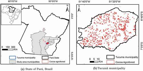
The data used in this work was obtained over an area in Pará in Brazil, comprising the municipalities highlighted in Figure 1 (Água Azul do Norte, Altamira, Canaã dos Carajás, Marabá, Ourilândia do Norte, Parauapebas, São Félix de Xingu and the Tucumã municipalities), during 2019. Note that the study area has a total of 292,822 km${ }^2$, while the Tucumã municipality only has 2,513 km${ }^2$, approximately 0.86% of the whole study area. According to Köppen’s climate classification map (Alcarde Alvares et al. 2013), the climate of the study area is equatorial monsoon (Am) in the southern and central sections, and equatorial rain forest, fully humid (Af) in the northern section. This area is drier than central Amazonia, with an annual rainfall of 2200–2800 mm, and has an annual mean temperature of over 26ºC.

Figure 1. Study area municipalities in Brazil. The locations of the cocoa agroforest areas identified inside the Embrapa’s MapCacao project are shown in red.

2.2. Sentinel-2 satellite imagery

The Sentinel-2 (S-2) satellite imagery with Level 1C product, was provided by Google Earth Engine (GEE) and made available by the European Space Agency (ESA). The S-2 mission includes twin satellites, the S-2A (launched in June 2015) and S-2B (launched in March 2017) which together provide global coverage of Earth’s land surface every 5 days (Marszalek et al. 2020; SUHET 2015). Through the multi-spectral instrument (MSI) carried on both satellites, 13 bands in the visible, near-infrared and short-wave infrared parts of the spectrum were acquired, each one representing the top of atmosphere reflectance, scaled by 10,000, and including radiometric and geometric corrections following the methods described in SUHET (2015).

Regarding the choice of satellite, Erasmi and Twele (2009) used both Landsat-7 and Envisat-ASAR images and states that natural forest and cocoa plantations are best recognized using only the optical dataset. As such, we opted to use optical images.

2.3. Datasets

2.3.1. 2019 Composite dataset (annual)

Our first dataset contains, as features, values that were obtained from an S-2 composite image built with all available images within 1 year of the given area. The compositing process, which consists of choosing for each pixel, and from a multi-temporal image stack in a specific period, the best possible unclouded pixel, was implemented in GEE and based on the computation of the median value among the available dates for each pixel (Cabral et al. 2003; Lopes, Leite, and Vasconcelos 2019; Corbane et al. 2020). After the compositing process, visible (blue, green and red) and near-infrared bands originally with a resolution of 10 m/pixel were re-sampled to 20 m/pixel using the mean value of the contributing original pixels, and jointly with the vegetation red edge, narrow infrared and the short-wave infrared bands rearranged in a final image (Lopes, Leite, and Vasconcelos 2019). The values obtained for each band were used to calculate several vegetation indexes: NDVI (Rouse et al. 1973), enhanced vegetation index (EVI) (Huete et al. 2002), green normalized vegetation index (GNDVI) (Candiago et al. 2015), plant senescence vegetation index (PSRI) (Ren, Chen, and An 2016), soil adjusted vegetation index (SAVI) (Huete 1988) and topographic effects reduction (TopR) (Cabral et al. 2011). NDVI and EVI are used as indicators of vegetation greenness and activity, and NDVI is also used for yield predictions and crop-type classification. EVI is more sensitive to high biomass conditions and contains empirically derived correction factors to correct background soil signal and reduce atmospheric effects. GNDVI measures the photosynthetic activity of the vegetation cover but is more sensitive to chlorophyll concentration. PSRI gives the value of plant senescence reflectance. SAVI is designed to minimize the confounding influence of soil spectral properties in the vegetation observation, when vegetation cover is poor and the soil surface is exposed. TopR (originally a ratio that used TM5 bands 5 and 2, which we adapted to a ratio between the Sentinel-2 bands 11 and 3) allows reducing topographic effects. We choose different vegetation indexes to improve the probability of spectral separation between vegetation classes, in particular the cocoa agroforest and forest.

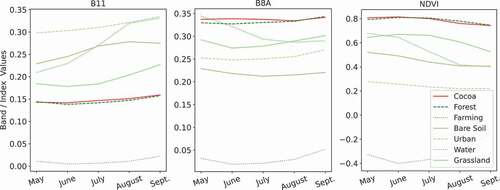
Figure 2 shows the median spectral signatures of the classes used in this dataset and suggests that all land cover types are separable using this approach, except for cocoa and forest. This is confirmed experimentally since our ML models are able to obtain a high accuracy in all classes except for these two.

Figure 2. Example of similar spectral signatures in the Annual dataset (obtained from a median composite of the study area using all selected images from May to September, 2019). The cocoa and forest land covers (highlighted in darker colours) have a nearly identical median spectral signature. Before plotting this graph, the features were rescaled, based on the band minimum and maximum for the dataset, to [0,1] for a better representation of all features within the same graph.

2.3.2. Monthly Time Series Dataset (MTS)

For our second dataset, we applied the same process as the Annual dataset to each month, from May to September, creating a total of five datasets (containing the values from the satellite bands and the indices) that were then merged into a single multivariate TS dataset. This approach has the advantage of allowing the models to learn the evolution of the spectral signatures of the classes over time, increasing the chances of learning the differences between the land cover types. It also has the downside of being a more noisy dataset and not guaranteeing that good-quality pixels exist in every month, which is the reason for our dataset containing only 5 months.

The improvement in the separability of the land cover types can be seen by comparing Figure 2 with Figure 3. While in the Annual dataset cocoa and forest have very similar spectral signatures, Band 8A in the MTS dataset suggests that these classes may be separable. This is also confirmed experimentally, since our ML models separate these two classes more easily, compared to using the Annual dataset.

Figure 3. Median values of each land cover type in each month. While Band 11 and NDVI do not show a good separability between the cocoa and forest classes, Band 8A suggests that these classes may be separable.

2.3.3. Extended MTS dataset (EMTS)

For our third dataset, we added the results of the following techniques to the MTS dataset, creating the EMTS dataset. It should be noted that the TS dataset is first normalized using the values of each feature in the whole training dataset and then the remaining techniques are applied to each sample individually:

Normalization: In each run, the program calculates the mean and standard deviation of each feature in the training set. Then, each sample (in the training and test sets) is normalized using the standard score technique;

Differencing: By applying this technique, we intend to extract additional information from the features by comparing the values in two consecutive months. For each feature, we calculate the difference by subtracting the value in each month by the value in the previous month, resulting in four new features for each band/index;

Trend: A linear regression classifier is fit to each sample and each band/index values individually (i.e. it is fit to the five values read in each feature) and the slope of the resulting line is added as a feature to the dataset;

Maximum and Minimum: For each band/index, we add the minimum and maximum values as additional features;

Peaks and Troughs: For each band/index, the number of peaks and troughs are added as two additional features. A month is considered a peak or a trough if both the previous and next values are, respectively, lower or higher than the current value.

2.3.4. Tucumã Time Series Dataset (TTS)

We use a fourth dataset, exclusively to validate the models that were trained using the EMTS dataset. Conceptually, the TTS dataset is equivalent to the EMTS dataset but uses different geographic bounds. The TTS dataset covers the whole Tucumã municipality, highlighted in Figure 1. This dataset was built in the same manner as the EMTS but, using only the S-2’s images over the tile 22MDT. The main difference between the TTS and the previous dataset is that, as we will see in the next section, the EMTS dataset covers a larger area (the whole study area) but only contains a sparse number of pixels. Meanwhile, the TTS dataset contains all pixels obtained from the satellite imagery above this municipality, leading to a much larger dataset that may contain noisier pixels (e.g. due to clouds) while only using 0.86% of the study area.

2.4. Reference data

This work uses a total of three datasets to train and test ML models and a fourth dataset that is used only for validation due to its large size. The pixels from the Annual, MTS and EMTS datasets have labels based on true class values and the TTS dataset has labels based on MapBiomas (collection5) map (2019)’s labels and the cocoa agroforest data collected by participatory mapping in the Embrapa’s MapCacao project, which is not included in MapBiomas. The features of the datasets are described in Table 1 and the number of pixels of each land cover type in Table 2.

Table 1. Total number of features used in each dataset.

Dataset	No. of Sentinel-2 bands	No. of indices	No. of composites	No. of temporal features	Total
Annual	13	6	1	0	19
MTS	13	6	5	0	95
EMTS	13	6	5	9^a	266
TTS	13	6	5	9^a	266

^aSee Section 2.3.3: For each band/index, we use the value in each month to calculate nine additional features.

Table 2. Total number of pixels in each class and pixels used for training/validation, in each dataset. Note that the TTS dataset is used exclusively for validation.

Dataset	Cocoa agroforest	Forest	Farming	Bare soil	Urban	Water	Grassland	Total
Annual MTS	700	707	457	322	195	188	50	2619
EMTS	490/210	495/212	320/137	225/97	136/56	132/56	35/15	1833/786
TTS	374,354	773,664	5,168,136	—	23,947	28,210	4950	6,373,261

For the creation of the MTS and EMTS datasets, we limited the datasets to the 2619 pixels that were labelled and available in the study area over the 5 months. We limit the Annual dataset to the same pixels, for a fair comparison between classifiers.

We use both bands and vegetation indices to collect training data (spectral values) for each cover type to build the datasets. Cocoa agroforest samples were obtained using the cocoa polygons identified in the project Embrapa’s MapCacao developed to Pará state, using a methodology that combines RS data validated and constructed through participatory mapping (Venturieri et al. 2019), while the other cover samples were identified on pre-existing vegetation maps and Google Earth high-resolution images.

To evaluate the classification results in the Tucumã municipality, we use MapBiomas (collection5) map (2019). The MapBiomas methodology is a pixel-based classification of a Landsat-8 composite image containing, at the general level (level-1), six classes: forest, non-forest natural formation, farming, non-vegetated area, water and non-observed. At level-2 and level-3, MapBiomas contains 22 classes including forest formation, pasture, ‘river, lake and ocean’, soybean, grassland, other temporary crops and urban infrastructure. To obtain a better match between the MapBiomas labels and our dataset’s labels, we renamed the following labels: forest formation (forest); pasture (farming); river, lake and ocean (water); soy bean (farming); grassland (grassland); other temporary crops (farming), and urban infrastructure (urban). The data are available at a spatial resolution of 1 arc-second per pixel, approximately 30 m per pixel at the equator, and 0.5 ha (Landsat scale) Minimum Mapping Unit (MMU). In addition to the MapBiomas classes, the reference image displayed in Figure 4 includes the cocoa agroforest cover type, obtained in the Embrapa’s MapCacao project. MapBiomas (collection5) map (2019) has a 97.6% accuracy on the level-1 classes in Amazonia, which gives this map a good reliability to be used for validation.

Figure 4. Reference image for the municipality of Tucumã. This image was obtained using the data for the year of 2019 available on MapBiomas (collection 5) map and the cocoa agroforest data collected by participatory mapping in the Embrapa’s MapCacao project, which is not included in MapBiomas. A section of the map is shown on the left to illustrate the similarity between the forest and cocoa agroforest land cover types.

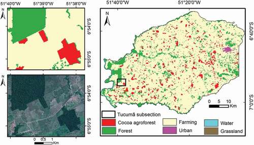
Tucumã was selected due to being the only municipality that had all cocoa agroforest labelled (Venturieri et al. 2019). It should be noted that, for training the classifier, samples were collected inside all the study areas, but the cocoa samples are located only in Tucumã and São Félix de Xingu, due to being the areas where cocoa was identified (see Figure 1). It should also be noted that the training dataset has 1833 pixels (70% of the EMTS dataset) and the TTS dataset has a total of 6,373,261 pixels (see Table 2).

2.5. Methodology

We attempt to improve the separation of cocoa agroforest from forest, while also training classifiers that can identify other classes, although the accuracy on the other classes is not reported. We opted not to merge classes in the training data since related work (Hoffmann, Kwok, and Compton 2001; Chen et al. 2022) states that the use of latent subclasses helps to build the robustness of ML models. We obtain training pixels from the whole study area (Figure 1) so that we can compare the robustness of the ML models when applied to an area different from the one used to obtain training data.

We use several well-known classifiers, including the state-of-the-art classifiers XGBoost and ROCKET, to show that our results are general across several classifiers and not specific to one particular kind of classifier. Each experiment is repeated 30 times, using different partitions of the datasets for training and testing the models, then statistical significance is determined with the nonparametric Kruskal-Wallis $H$-test (from the scipy Python library (Virtanen et al. 2020)) at $p<0.01$. To ensure the reproducibility of these simulations, we use the number of the run as a random seed to assemble the training and test partitions, and each classifier uses that same number as the random_state argument. Except for this argument, all classifiers use the default parameters defined in their respective implementations. Although we are aware that the lack of parameter-tuning may lead to sub-optimal results, even using the default parameters, this work shows the importance of TS data in the separation of similar cover types. It should be noted that, except for the ROCKET algorithm, these classifiers were not built for TS datasets but, due to the low number of features within the datasets, we decided that the following classifiers should be tested:

M3GP: The multidimensional multiclass genetic programming with multidimensional populations (M3GP) (Muñoz, Silva, and Trujillo 2015) algorithm is based on genetic programming and performs both implicit feature selection and explicit feature construction, creating a set of features for increasing the learning capability of another classifier. This implementation is available at M3GP Repository (2019);

Multilayer Perceptron Classifier: The multilayer perception (MLP) (Noriega 2005) classifier is a feedforward artificial neural network ML algorithm. We used the scikit-learn (Pedregosa et al. 2011) implementation of this classifier;

Ridge: The ridge classifier (Grüning and Kropf 2006) is a simple regression algorithm that is used by the ROCKET algorithm. We used the scikit-learn scikit implementation of this classifier;

Random Forest: The random forest (RF) (Breiman 2001) classifier is an ensemble algorithm that uses the majority vote of a set of decision trees to make predictions. We used the scikit-learn (Pedregosa et al. 2011) implementation of this classifier;

ROCKET: The ROCKET is a state-of-the-art algorithm that uses random convolution kernels to increase the dimensionality of a dataset and, together with ridge, a simple regression classifier, obtains state-of-the-art accuracy. We used the authors’ implementation (Dempster, Petitjean, and Webb 2020; ROCKET Repository 2020) with a modification to accept a random seed, allowing the reproducibility of the simulations;

XGBoost: The extreme gradient boosting, or XGBoost (×GB) (Chen and Guestrin 2016) classifier, is a state-of-the-art ensemble algorithm that uses a set of decision trees and an optimized gradient boost to minimize errors. We used the XGB implementation from the xgboost Python library;

M3GP+XGBoost: In the previous work (Batista et al. 2021), M3GP was used to create a set of features (using the training data) that, when added to the whole dataset, improved the test accuracy of the models. This effect was particularly noticeable when training a model in pixels from one image and applying it to a different image, showing the robustness of these new features (Batista and Silva 2020). We used this combination of algorithms where, in each run, M3GP creates a different set of features that are then added to the dataset that XGB uses to train and test a classification model. Then, we compare the M3GP+XGB results with those obtained by the XGB models.

3. Results and discussion

3.1. 2019 composite dataset (annual)

The first experiment in this work is the training and application of the ML classifiers in the Annual dataset. The median test overall accuracy (OA), producer’s accuracy (PA) and UA for this dataset are seen on Table 3, and the median test confusion matrices, obtained over 30 runs using the XGB and M3GP+XGB classifiers, is seen on Figure 5. Note that the confusion matrices are normalized so that the percentages in each row/class reflect real-world percentages, based on the percentages of each land cover type in the Tucumã municipality.

Figure 5. Confusion matrices (as percentages) for the XGB and M3GP+XGB test cases on the Annual, MTS and EMTS datasets. Median of 30 runs, each row is normalized to the percentage of each cover type in the TTS dataset to simulate real-world percentages.

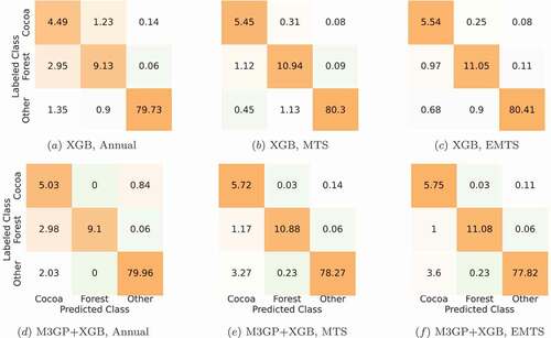
Table 3. Median PA, UA and OA (all values as percentages) of each set of 30 models trained on the EMTS dataset when applied to the TTS dataset.

	M3GP	MLP	RF	Ridge	ROCKET	XGB	M3GP+XGB
Annual dataset
Test OA%	85.18	74.68	83.97	71.31	84.48	85.56	88.42
Cocoa PA/UA%	77.6/66.7	53.9/47.4	68.8/76.7	49.4/32.4	70.9/75.0	73.7/76.4	74.4/85.7
Forest PA/UA%	73.2/80.7	57.0/67.5	75.0/68.4	50.4/73.1	74.6/71.0	77.0/75.2	100.0/75.0
Other PA/UA%	96.4/98.1	98.6/94.8	98.1/96.7	98.6/93.1	97.9/97.4	98.3/97.3	92.1/97.5
MTS dataset
Test OA%	89.38	84.67	92.11	83.59	91.60	94.40	94.66
p-value (vs Annual)	0.0000	0.0000	0.0000	0.0000	0.0000	0.0000	0.0000
Cocoa PA/UA%	87.9/76.0	70.1/84.8	85.0/89.0	70.3/81.9	83.3/89.0	89.9/92.9	85.8/97.4
Forest PA/UA%	80.7/87.7	78.9/66.7	89.3/85.4	74.9/67.2	88.2/84.4	91.9/90.1	99.0/89.6
Other PA/UA%	96.1/98.4	98.1/97.5	98.6/97.5	97.4/94.0	98.3/97.5	98.8/97.9	98.4/95.5
EMTS dataset
Test OA%	88.93	93.13	92.81	89.44	93.38	95.17	94.78
p-value (vs MTS)	0.0758	0.0000	0.0319	0.0000	0.0000	0.0208	0.7782
Cocoa PA/UA%	84.6/78.3	87.7/91.2	85.9/90.5	79.4/90.0	87.2/91.9	90.8/94.3	85.5/97.9
Forest PA/UA%	81.5/85.1	90.1/87.3	90.5/86.8	85.9/77.8	91.3/87.7	93.1/91.0	98.5/91.3
Other PA/UA%	95.8/97.0	97.8/97.8	98.5/97.5	98.0/96.4	98.1/97.8	98.6/98.1	98.7/94.9

The cases with p-value <0.01 are highlighted in green when the OA is improved. The PA and UA with values over 90% are highlighted in blue.

In order to understand where the classifiers are failing, we calculated the test PA and UA for the cocoa and forest classes and merge all other classes into a class named ‘Other’. We can see that even the classifiers with the lowest median OA obtain high value of PA/UA on the other classes, but all classifiers fail to obtain high PA/UA in the cocoa and forest classes. Except for the M3GP+XGB classifier, these values have a maximum of 77.6%. Using the M3GP+XGB classifier, although the values for PA/UA are improved, they are not as good as the other classes.

By analysing the confusion matrices of the XGB and M3GP+XGB classifiers (Figure 5), we can see that, when using the XGB classifier, there is some confusion between the cocoa and forest land cover types but, these classes are barely mistaken with the other classes within the dataset. These two classes are easily mistaken with each other, which is expected given the spectral radiometric similarity issues that have been previously established. When using the M3GP+XGB classifier, the results show that the features created by M3GP help to tackle the biggest issue in this dataset, raising the median PA on the forest class to 100.0% while also improving the median UA on the cocoa class. However, this improvement reduced the PA of other classes that are not more frequently mistaken as cocoa.

3.2. Monthly Time Series Dataset (MTS)

The second experiment in this work is the training and application of the ML classifiers in the MTS dataset. The accuracy values and $p$-values can be seen in Table 3 and the test confusion matrices for the XGB and M3GP+XGB classifiers in Figure 5.

The first thing to note is that, just from using time series, there is a clear improvement in test OA, in comparison to using the Annual dataset, in all classifiers (with a $p$-value of 0.0000). Once again, we look more closely at the classifiers with the best results, XGB and M3GP+XGB. When compared to the Annual dataset, besides improving its OA, XGB also improves the median PA/UA on the cocoa and forest classes to values over 90%, except for the cocoa PA. The problems identified in the M3GP+XGB classification in the Annual dataset persist in the MTS dataset. Although its OA is on par with the XGB, the PA/UA on the cocoa and forest classes are dissimilar. As expected from the PA/UA, the confusion matrices indicate a lower confusion among these three classes in the MTS dataset, when compared to the Annual dataset. However, M3GP+XGB seems to be mistaken cocoa for the other classes more frequently.

These results were expected for the reasons mentioned before: TS datasets contain more information about the land cover types, facilitating their separation. Generally speaking, a higher OA does not mean that all classes have better accuracy since the accuracy can go up in some classes and decrease in others. However, in this particular case, all the classifiers improved their performance by using the MTS dataset.

3.3. Extended MTS Dataset (EMTS)

The third experiment in this work is the training and application of the ML classifiers in the EMTS dataset. The accuracy values and $p$-values can be seen in Table 4 and the test confusion matrices for the XGB and M3GP+XGB classifiers in Figure 4.

Table 4. Median PA, UA and OA (all values as percentages) of each set of 30 models trained on the EMTS dataset when applied to the TTS dataset.

	Cocoa		Forest		Other
Model	PA	UA	PA	UA	PA	UA	OA
M3GP	11.99	18.43	40.08	56.29	91.71	96.15	82.07
MLP	86.38	20.53	22.35	61.86	84.92	98.07	77.43
RF	79.09	22.64	35.51	52.96	86.26	98.22	79.53
Ridge	94.32	10.92	0.09	22.46	59.40	98.79	54.25
XGB	79.81	25.63	39.78	60.07	88.50	98.12	81.78
M3GP+XGB	76.52	28.25	42.88	57.25	89.51	98.07	82.91

In comparison with the MTS dataset, three of the seven classifiers improved their test OA with a p-value <.01, while XGB improved with a p-value <.05. In this case, the use of the M3GP algorithm for feature construction seems to have neutral or negative impact on the accuracy of the XGB classifier. This may be due to the M3GP algorithm not being optimized for the large number of features that exist in this dataset (see Table 1), in comparison with the previous experiment. However, other GP methods have shown good results when dealing with a large number of features (Idris, Khan, and Lee 2012; Rodrigues, Batista, and Silva 2020; Pei et al. 2019; Rodrigues et al. 2022) and, since GP produced simple models that can be used for fast classification of images (when compared to other well-known methods such as deep learning), this is still a method worth pursuing for dealing with TS datasets.

In terms of accuracy per class obtained with XGB (Table 3) we can see that, compared to the MTS dataset, the PA/UA of the cocoa and forest classes is slightly improved, but there is no statistical significance to allow hard conclusions. In terms of confusion matrices, the conclusions are equal to those on the MTS dataset. This may indicate that, unlike other algorithms, the XGB algorithm is able to extract enough information from the MTS dataset.

3.4. Tucumã Time Series Dataset (TTS)

In the fourth experiment, we apply all the models previously trained using the EMTS dataset, except the ROCKET models, in the TS produced using images of Tucumã, and calculate their median OA, PA and UA (see Table 4). We use MapBiomas to calculate the models accuracy. This map is based in Landsat-8 imagery with 30 m pixels and a correction to 0.5 ha MMU. To compensate for this difference in resolution, after our models classify each image, the resulting map is smoothed using a 3 × 3 majority filter.

The ROCKET algorithm was excluded from this experiment since it generates 10,000 features from the input image, essentially generating an amount of data that we are unable to process¹. Since, in the previous experiments, the XGB and M3GP+XGB classifiers had the highest median OA (Table 3), we selected the best model from each classification algorithm to classify the imagery, obtaining two maps (see Figure 7).

Note that the forest and cocoa agroforest accuracy on the TTS dataset is lower in comparison to the EMTS dataset. We have two hypotheses for this accuracy reduction. First, although we obtained the training data from a larger area, the models can be affected by the radiometric differences between images, leading to lower accuracy values in validation datasets obtained from satellite images with low or no representation in the training data. Second, we selected all satellite pixels over Tucumã, leading to the images including small clouds scattered over the municipality. This noise impacts the values read by the satellite bands, which misleads the classification algorithm.

3.4.1. XGBoost classifier

The median confusion matrix and the confusion matrix from the run with the highest OA (i.e. the best run) when using the XGB classifiers on the Tucumã municipality can be seen in Figure 6 and the municipality classified in the best run can be seen in Figure 7. From the confusion matrices, we can comment that:

Figure 6. Confusion matrices (as percentages) obtained by using the XGB and M3GP+XGB in the Tucumã imagery. The confusion matrices are normalized to 100.

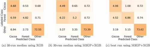
Figure 7. Classification of the municipality of Tucumã (TTS dataset), performed by the (a) XGB and (b) M3GP+XGB models with the highest OA.

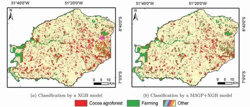
Cocoa is equally mistaken as forest and as some of the other classes. The issue with the forest class was already present in the previous sections and may be associated with the inclusion of non-cocoa trees in the cocoa pixels since trees are known to co-habit inside cocoa agroforest polygons. Given the large amount of pixels in the border between cocoa polygons and farming, the misclassification of cocoa as one of the other classes may come from the proximity with these areas;

Forest is frequently misclassified as cocoa. Given the improvements in the accuracy on the EMTS dataset, it was unexpected that forest would be so easily mistaken with cocoa. Although some misclassified pixels can be associated with the pixels in the borders between cocoa and forest, the biggest issue may be the new plantations of cocoa in the Tucumã municipality. The new cocoa plantations are mixed with forest trees. When the cocoa trees are still in the early growing stage, these areas are mostly defined by the non-cocoa trees that are planted beforehand and that is why there is such a spectral confusion between these two classes.

3.4.2. M3GP+XGB classifier

Besides reducing the dissimilarity between the PA/UA of the forest and cocoa classes, performing feature construction using the M3GP did not bring any improvements worthy of discussion. However, at least two interesting hyper-features were created in the run with the best test OA.

As seen in Figure 6, this run has a better separation of the cocoa and forest cover types when compared to the median run. The M3GP algorithm produced 25 new features from the 266 features in the EMTS dataset. Out of them, 17 features are present in the original dataset, and 8 features are the expressions in Table 5.

Table 5. M3GP features used to classify the Tucumã imagery in the M3GP+XGB run with the best OA.

ID	Mathematical expression
HF1	(B6T/B11Jul) + B1’Aug
HF2	NDVIAug * NDVIAug
HF3	SAVIT * SAVIAug
HF4	B2T - B3T + (B4min/B11Jul)
HF5	B1’Aug - B8AJun
HF6	B2T - B1T + B12max
HF7	B6P/B4max
HF8	SAVIP * B2P/B3Aug + B8AT + NDVIAug - EVI’Jun * B9’Aug * B1’Sep * (SAVIP - B10Jun)

Bn_T = Number of Troughs on band n; Bn_P = Number of Peaks; Bn‘x = Difference between the values on month x and on month x-1.

Taking into consideration the distribution of values of each hyper-feature (see Figure 8, the most relevant features seem to be HF2, HF3 and HF7. HF2 is the squared NDVI value for August, HF3 multiplies the SAVI trend by its value in August and HF7 divides the number of peaks in B6 with the maximum value in B4. Although none of these features perfectly separates the two classes, the median forest value in HF2 is in the interquartile range border of the cocoa class and HF7 indicates a higher variance of B6 in the cocoa pixels (leading to a higher number of peaks).

Figure 8. Distribution of values using each hyper-feature on Table 5. The black line indicates the median value and the grey lines the interquartile range.

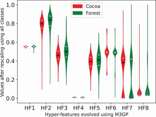
It is also worth mentioning that the M3GP seems to prefer the August bands. These eight hyper-features use a total of 28 features, from which 14 are associated with a month (e.g. B1’${ }_{Aug}$). Out of those features, eight are associated with August. It is also worth pointing out that, out of these eight hyper-features, three explicitly use bands from different months, which may lead to future work on multi-temporal indices.

3.5. Comparison with related works

In this section, we compare our methodology with the one reported by other authors in the classification of cocoa agroforest and full-sun cocoa. The comparisons are based on the information displayed in Table 6. First, we want to state that all other works perform a single run on the datasets, which may lead to inaccurate estimates of the models’ expected accuracy, while we report the 30-runs median accuracy.

Table 6. Comparison with related work. The first column includes the number of runs presented in each work, the metrics used to evaluate accuracy (overall accuracy (OA), producer’s accuracy (PA), user’s accuracy (UA), Kappa coefficient (K) and p-value) and the size of the training (Tr.) and validation (Val.) sets.

	Validation method	Imagery	Cocoa type	Data type	Texture analysis	OA and cocoa accuracy (OA/PA/UA)%	Classification methods
This work	30-runs median OA/PA/UA/p 1,833 pixels (Tr. set) 768 pixels (Val. set) 6,373,261 pixels (TTS)	Sentinel-2A	Agroforest	Composite Timeseries (6 composites)	––	Composite Val. 85.6/73.7/76.4 TS Val. 95.2/90.8/94.3 TS Tucumã Imagery 82.9/76.5/28.3	Composite/TS XGBoost Tucumã/M3GP+XGB
Abu et al. (2021)	Single-run PA/UA 17,277 pixels (Tr. set) 1,919 pixels (Val. set)	Sentinel-1 Sentinel-2	Agroforest	Composite	GLCM	–/82.9/62.2	Optimized Random Forests
Benefoh et al. (2018)	Single-run OA/PA/UA/K 350 polygons (Tr. set) 182 polygons (Val. set) 25,267 pixels (total)	Landsat-5 Landsat-7 Landsat-8	Fullsun Agroforest	Composite	––	Overall Acc.: 89 Full-sun: 97/96 Agroforest: 86/95	Maximum Likelihood Classifier and K-means
Numbisi, Van Coillie and De Wulf (2019)	Single-run OA/PA/UA 70% pixels (Tr. set) 30% pixels (Val. set) Unknown No. Pixels	RapidEye Sentinel-1	Agroforest	Single Image/RapidEye Time Series/Sentinel-1 (10 dates)	GLCM	RapidEye 81.0/66.1/66.4 Sentinel-1 88.8/95.6/85.8	Random Forests
Twele et al. (2006)	Single-run OA/PA/K Unknown No. Pixels	Landsat-7	Agroforest	Single Image	––	83.2/85.0/–	Maximum Likelihood Classifier
Erasmi and Twele (2009)	Single-run OA/PA/K Unknown No. Pixels	Landsat-7 Envisat	Unspecified	Time Series/6 dates (Envisat) plus 2 dates (Landsat-7)	SAR-based texture measures	89/98/–	Nearest Neighbour Classifier

In terms of satellite imagery, two well-known issues in the detection of cocoa are the cloud coverage in the tropical regions and the presence of taller trees that make shade on the cocoa trees. Nevertheless, all of the mentioned works use optical imagery. Benefoh et al. (2018) obtained very high PA/UA values for the full-sun cocoa, i.e. cocoa farms without other trees making shade, facilitating the detection of cocoa. Although Erasmi and Twele (2009) do not specify the kind of cocoa used in their study, Smiley and Kroschel (2010) state that, during the time both works were written, the cocoa agroforest plantations in the area (Palolo valley, Indonesia) were progressing to full-sun cocoa. Assuming this is the case, this possibly explains the high reported PA value.

Abu et al. (2021) uses a composite containing both optical and radar imagery and Gray-Level Co-Occurrence Matrix (GLCM) metrics, but the reported PA/UA average is lower than in our composite dataset (Annual). Numbisi, Van Coillie, and De Wulf (2019) use a TS dataset made with 10 dates, using radar imagery and GLCM metrics. The PA/UA values on the cocoa agroforest are similar to our results.

Lastly, in our work, we compare the results of several models in composite and time-series data. Table 6 indicates that works that use uni-temporal data (i.e. single composites or single images) generally have lower OA/PA/UA values, giving a higher emphasis on the benefits of using TS data.

4. Conclusions

The main objective of this work is to study the use of short TS data for the classification of cocoa agroforest and forest land cover types. Given the clear success of the TS classification, this work also includes the preprocessing of the TS datasets, which allows the accuracy to be improved even further with half of the used ML classifiers.

Our methodology is compared with the ones used by other authors in the separation of cocoa agroforest and full-sun cocoa from the forest land cover type. We observe that our results may be more accurate than the related work even though we only use optical imagery. This improvement might also be derived from the classification algorithm used (×GB), which is normally more powerful than the popular RF algorithm. However, using the XGB algorithm for RS data is a rarer choice.

Since the XGB classifier obtained the best results in our datasets, we apply the models to TS made using satellite imagery over the Tucumã municipality. This includes two experiments: training the XGB models directly on the EMTS dataset and training the models after performing feature construction using the M3GP algorithm.

The best results come from the models trained after performing feature construction. These models obtain a median PA/UA on the cocoa pixels of 76.52%/28.25%, indicating that this work should be further explored. Given the difference in results between the TTS and the EMTS datasets, this issue seems to be heavily related to the radiometric difference between the pixels from the area used to train the model and the pixels from this area, a well-known issue in the RS field. However, the XGB algorithm improved its accuracy when using the features created by the M3GP algorithm, indicating that these features have some robustness to these radiometric variations.

We consider that this work is relevant not only for this particular study case but also for the separation of any two land cover types with similar spectral signatures, such as the previous works mentioned in the introduction. For future work, we intend to continue studying the separability of land cover types, in particular cocoa and forest, and also cashew and forest, in an attempt to create machine learning models that are more robust to the radiometric variations across satellite images. In this work, we used the default parameters of the ML algorithms. We also plan on improving our results by improving our preprocessing techniques and tuning the model parameters. Given the results from the M3GP feature construction algorithm, we believe that future work should also explore the creation of multi-temporal indices.

Data availability

A section of the dataset used in this work is available at https://github.com/jespb/Cocoa_PublicDS. This dataset includes all classes, except for cocoa agroforest, since this data is proprietary. The MapBiomas data is available from MapBiomas (collection 5) map https://mapbiomas.org.

Acknowledgement(s)

We would also like to thank the technicians of Embrapa (Brazilian Agricultural Research Corporation), Ceplac (Executive Commission for the Cacao Crop Plan) and Emater (Technical Assistance and Rural Extension Company), and to rural producers for their support in the field work.

Disclosure statement

No potential conflict of interest was reported by the author(s).

Additional information

Funding

This work was partially supported by FCT through funding of LASIGE Research Unit (UIDB/00408/2020 and UIDP/00408/2020) and CEF [UIDB/00239/2020]; projects OPTOX [PTDC/CTA-AMB/30056/2017], INTERPHENO [PTDC/ASP-PLA/28726/2017] and GADgET [DSAIPA/DS/0022/2018]; PhD Grants [SFRH/BD/143972/2019 and 2021/05322/BD]. It also received funding from European Union’s Horizon 2020 Research and innovation programme under the Marie Sklodowska-Curie grant agreement No. 691053 [H2020-MSCA-RISE-2015 ODYSSEA project] and it was supported by the Embrapa’s MapCacao project (Project: Mapping of areas with cocoa plantations (Theobroma cacau L.) in the State of Pará - Mapcacau- Agreement SEDAP [SEI 21159.005419/2018-61].

Notes

1. A minimum of 762GB RAM per run, since each feature is a 3731 × 2676 matrix of 64-bit floats.

References

- Abu, I.-O., Z. Szantoi, A. Brink, M. Robuchon, and M. Thiel. 2021. “Detecting Cocoa Plantations in Côte d’Ivoire and Ghana and Their Implications on Protected Areas.” Ecological Indicators 129: 107863. doi:10.1016/j.ecolind.2021.107863.
- Akinyemi, F. O. 2013. “An Assessment of Land-Use Change in the Cocoa Belt of South-West Nigeria.” International Journal of Remote Sensing 34 (8): 2858–2875. doi:10.1080/01431161.2012.753167.
- Alcarde Alvares, C., J. Stape, P. Sentelhas, J. Gonçalves, and G. Sparovek. 2013. “Köppen’s Climate Classification Map for Brazil.” Meteorologische Zeitschrift 22 711–728 .
- Asare, R., B. Markussen, R. A. Asare, G. Anim-Kwapong, and A. Ræbild. 2018. “On-Farm Cocoa Yields Increase with Canopy Cover of Shade Trees in Two Agro-Ecological Zones in Ghana.” Climate and Development 11 (5): 435–445. doi:10.1080/17565529.2018.1442805.
- Asubonteng, K., K. Pfeffer, M. Ros-Tonen, J. Verbesselt, and I. Baud. 2018. “Effects of Tree-Crop Farming on Land-Cover Transitions in a Mosaic Landscape in the Eastern Region of Ghana.” Environmental Management 62 (3): 529–547. doi:10.1007/s00267-018-1060-3.
- Ayanlade, A. 2017. “Remote Sensing Vegetation Dynamics Analytical Methods: A Review of Vegetation Indices Techniques.” Geoinformatica Polonica 16 (2017): 7–17. doi:10.4467/21995923GP.17.001.7188.
- Batista, J. E. and S. Silva. 2020. “Improving the Detection of Burnt Areas in Remote Sensing Using Hyper-Features Evolved by M3gp.” In 2020 IEEE Congress on Evolutionary Computation (CEC) Glasgow, United Kingdom, 1–8.
- Batista, J. E., A. I. R. Cabral, M. J. P. Vasconcelos, L. Vanneschi, and S. Silva. 2021. “Improving Land Cover Classification Using Genetic Programming for Feature Construction.” Remote Sensing 13 (9): 1623. doi:10.3390/rs13091623.
- Benefoh, D., G. Villamor, M. Van Noordwijk, C. Borgemeister, W. Asante, and K. Asubonteng. 2018. “Assessing Land-Use Typologies and Change Intensities in a Structurally Complex Ghanaian Cocoa Landscape.” Applied Geography 99. doi:10.1016/j.apgeog.2018.07.016.
- Breiman, L. 2001. “Random Forests.” Machine Learning 45 (1): 5–32. doi:10.1023/A:1010933404324.
- Cabral, A., M. J. P. D. Vasconcelos, J. M. C. Pereira, É. Bartholomé, and P. Mayaux. 2003. “Multi-Temporal Compositing Approaches for SPOT-4 VEGETATION.” International Journal of Remote Sensing 24 (16): 3343–3350. doi:10.1080/0143116031000075936.
- Cabral, A., M. Vasconcelos, D. Oom, and R. Sardinha. 2011. “Spatial Dynamics and Quantification of Deforestation in the Central-Plateau Woodlands of Angola (1990–2009).” Applied Geography 31: 1185–1193. doi:10.1016/j.apgeog.2010.09.003.
- Candiago, S., F. Remondino, M. D. Giglio, M. Dubbini, and M. Gattelli. 2015. “Evaluating Multispectral Images and Vegetation Indices for Precision Farming Applications from UAV Images.” Remote Sensing 7 (4): 4026–4047. doi:10.3390/rs70404026.
- Chen, T. and C. Guestrin. 2016. “Xgboost: A Scalable Tree Boosting System.” In Proceedings of the 22nd ACM SIGKDD International Conference on Knowledge Discovery and Data Mining, KDD ‘16, 785–794. New York, NY: ACM.
- Chen, M., D. Fu, A. Narayan, M. Zhang, Z. Song, K. Fatahalian, and C. Ré. 2022. “Perfectly Balanced: Improving Transfer and Robustness of Supervised Contrastive Learning.”
- Corbane, C., P. Politis, P. Kempeneers, D. Simonetti, P. Soille, A. Burger, M. Pesaresi, et al. 2020. ”A Global Cloud Free Pixel- Based Image Composite from Sentinel-2 Data”. Data in Brief 31: 105737. doi:10.1016/j.dib.2020.105737.
- Csillik, O., M. Belgiu, G. P. Asner, and M. Kelly. 2019. “Object-Based Time-Constrained Dynamic Time Warping Classification of Crops Using Sentinel-2.” Remote Sensing 11 (10): 1257. doi:10.3390/rs11101257.
- Dempster, A., F. Petitjean, and G. I. Webb. 2020. “Rocket: Exceptionally Fast and Accurate Time Classification Using Random Convolutional Kernels.” Data Mining and Knowledge Discovery 34 (5): 1454–1495.
- Domingos, P. 2012. “A Few Useful Things to Know About Machine Learning.” Communications of the ACM 55 (10): 78–87.
- Duguma, B., J. Gockowski, and J. Bakala. 2001. “Smallholder Cacao (Theobroma Cacaolinn.) Cultivation in Agroforestry Systems of West and Central Africa: Challenges and Opportunities.” Agroforestry Systems 51 (3): 177–188. doi:10.1023/A:1010747224249.
- Erasmi, S. and A. Twele. 2009. “Regional Land Cover Mapping in the Humid Tropics Using Combined Optical and SAR Satellite Data—A Case Study from Central Sulawesi, Indonesia.” International Journal of Remote Sensing 30 (10): 2465–2478. doi:10.1080/01431160802552728.
- FAO. 2018. “Faostat Statistical Database.” https://www.fao.org/faostat/en/#data/QCL
- Grüning, M. and S. Kropf. 2006. ”A Ridge Classification Method for High-Dimensional Observations.” In From Data and Information Analysis to Knowledge Engineering, edited by M. Spiliopoulou, R. Kruse, C. Borgelt, A. Nürnberger, and W. Gaul, 684–691. Berlin Heidelberg: Springer.
- Hoffmann, A., R. Kwok, and P. Compton. 2001. “Using Subclasses to Improve Classification Learning.” In European Conference on Machine Learning 2001 September 5, 203–213. Berlin, Heidelberg: Springer.
- Huete, A. R. 1988. “A Soil-Adjusted Vegetation Index (Savi).” Remote Sensing of Environment 25 (3): 295–309. doi:10.1016/0034-4257(88)90106-X.
- Huete, A., K. Didan, T. Miura, E. Rodriguez, X. Gao, and L. Ferreira. 2002. “Overview of the Radiometric and Biophysical Performance of the MODIS Vegetation Indices.” Remote Sensing of Environment 83 (1–2): 195–213. doi:10.1016/S0034-4257(02)00096-2.
- Idris, A., A. Khan, and Y. S. Lee. 2012. “Genetic Programming and Adaboosting Based Churn Prediction for Telecom.” In 2012 IEEE international conference on Systems, Man, and Cybernetics (SMC) Seoul, South Korea, 1328–1332. IEEE.
- Kottek, M., J. Grieser, C. Beck, B. Rudolf, and F. Rubel. 2006. “World Map of the Köppen-Geiger Climate Classification Updated.” Meteorologische Zeitschrift 15 (3): 259–263. doi:10.1127/0941-2948/2006/0130.
- Kussul, N., M. Lavreniuk, S. Skakun, and A. Shelestov. 2017. “Deep Learning Classification of Land Cover and Crop Types Using Remote Sensing Data.” IEEE Geoscience and Remote Sensing Letters 14 (5): 778–782. doi:10.1109/LGRS.2017.2681128.
- Kuzucu, A. and F. Balcik. 2017. “Testing the Potential of Vegetation Indices for Land Use/cover Classification Using High Resolution Data.” ISPRS Annals of Photogrammetry, Remote Sensing and Spatial Information Sciences IV-4/W4: 279–283. doi:10.5194/isprs-annals-IV-4-W4-279-2017.
- Lopes, C., A. Leite, and M. J. Vasconcelos. 2019. “Open-Access Cloud Resources Contribute to Mainstream REDD+: The Case of Mozambique.” Land Use Policy 82: 48–60. doi:10.1016/j.landusepol.2018.11.049.
- M3GP Repository. 2019. “M3GP: Python Implementation.” github.com/jespb/Python-M3GP
- MapBiomas (collection5) map. 2019. “MapBiomas.” https://mapbiomas.org/atbd-3
- Marszalek, M., M. Lösch, M. Körner, and U. Schmidhalter. 2020. “Multi-Temporal Crop Type and Field Boundary Classification with Google Earth Engine.”
- Muñoz, L., S. Silva, and L. Trujillo. 2015. “M3gp – Multiclass Classification with GP.” In ,Lecture Notes in Computer Science edited by Machado, Penousal, Heywood, Malcolm I., McDermott, James, Castelli, Mauro, García-Sánchez, Pablo, Burelli, Paolo, Risi, Sebastian, Sim, Kevin. 78–91. Copenhagen, Denmark: Springer International Publishing.
- Noriega, L. 2005. “Multilayer Perceptron Tutorial.” School of Computing. Staffordshire University.
- Numbisi, F. N., F. M. B. Van Coillie, and R. De Wulf. 2019. “Delineation of Cocoa Agroforests Using Multiseason Sentinel-1 Sar Images: A Low Grey Level Range Reduces Uncertainties in Glcm Texture-Based Mapping.” ISPRS International Journal of Geo-Information 8 (4): 179. doi:10.3390/ijgi8040179.
- Pedregosa, F., G. Varoquaux, A. Gramfort, V. Michel, B. Thirion, O. Grisel, M. Blondel, et al. 2011. ”Scikit-Learn: Machine Learning in Python.” Journal of Machine Learning Research 12 (Oct): 2825–2830.
- Pei, W., B. Xue, L. Shang, and M. Zhang. 2019. “New Fitness Functions in Genetic Programming for Classification with High-Dimensional Unbalanced Data.” In 2019 IEEE Congress on Evolutionary Computation (CEC) Wellington, New Zealand, 2779–2786. IEEE.
- Peña-Barragán, J. M., F. López-Granados, L. Garca-Torres, M. Jurado-Expósito, M. S. de la Orden, and A. Garca-Ferrer. 2008. “Discriminating Cropping Systems and Agro-Environmental Measures by Remote Sensing.” Agronomy for Sustainable Development 28 (2): 355–362. doi:10.1051/agro:2007049.
- Pereira, S. C., C. Lopes, and J. Pedro Pedroso. 2022. “Mapping Cashew Orchards in Cantanhez National Park (Guinea-Bissau).” Remote Sensing Applications: Society and Environment 26: 100746. doi:10.1016/j.rsase.2022.100746.
- Polykretis, C., M. G. Grillakis, and D. D. Alexakis. 2020. “Exploring the Impact of Various Spectral Indices on Land Cover Change Detection Using Change Vector Analysis: A Case Study of Crete Island, Greece.” Remote Sensing 12 (2): 319. doi:10.3390/rs12020319.
- Ren, S., X. Chen, and S. An. 2016. “Assessing Plant Senescence Reflectance Index-Retrieved Vegetation Phenology and Its Spatiotemporal Response to Climate Change in the Inner Mongolian Grassland.” International Journal of Biometeorology 61 (4): 601–612. doi:10.1007/s00484-016-1236-6.
- ROCKET Repository. 2020. “ROCKET: Python Implementation.” github.com/angus924/rocket
- Rodrigues, N. M., J. E. Batista, and S. Silva. 2020. “Ensemble Genetic Programming Hu, Ting, Lourenço, Nuno, Medvet, Eric, Divina, Federico.” In Lecture Notes in Computer Science , 151–166. Seville, Spain: Springer International Publishing.
- Rodrigues, N. M., J. E. Batista, W. La Cava, L. Vanneschi, and S. Silva. 2022. ”Slug: Feature Selection Using Genetic Algorithms and Genetic Programming.” In Genetic Programming, edited by E. Medvet, G. Pappa, and B. Xue E. Medvet, G. Pappa, and B. Xue 68–84. Cham: Springer International Publishing.
- Rouse, J. W., R. H. Haas, J. A. Schell, and D. W. Deering. 1973. “Monitoring Vegetation Systems in the Great Plains with Erts.”
- Rujoiu-Mare, M.-R. and B.-A. Mihai. 2016. ”Mapping Land Cover Using Remote Sensing Data and Gis Techniques: A Case Study of Prahova Subcarpathians.” Procedia Environmental Sciences 32: 244–255, ECOSMART - Environment at Crossroads: Smart Approaches for a Sustainable Development. doi:10.1016/j.proenv.2016.03.029.
- Rujoiu-Mare, M.-R., B. Olariu, B.-A. Mihai, C. Nistor, and I. Săvulescu. 2017. “Land Cover Classification in Romanian Carpathians and Subcarpathians Using Multi-Date Sentinel-2 Remote Sensing Imagery.” European Journal of Remote Sensing 50 (1): 496–508. doi:10.1080/22797254.2017.1365570.
- Schroth, G., E. Garcia, B. W. Griscom, W. G. Teixeira, and L. P. Barros. 2015. “Commodity Production as Restoration Driver in the Brazilian Amazon? Pasture Re-Agro-Forestation with Cocoa (Theobroma Cacao) in Southern Pará.” Sustainability Science 11 (2): 277–293. doi:10.1007/s11625-015-0330-8.
- Shao, Y., R. S. Lunetta, B. Wheeler, J. S. Iiames, and J. B. Campbell. 2016. “An Evaluation of Time-Series Smoothing Algorithms for Land-Cover Classifications Using Modis-NDVI Multi-Temporal Data.” Remote Sensing of Environment 174: 258–265. doi:10.1016/j.rse.2015.12.023.
- Smiley, G. and J. Kroschel. 2010. “Yield Development and Nutrient Dynamics in Cocoa-Gliricidia Agroforests of Central Sulawesi, Indonesia.” Agroforestry Systems 78: 97–114. doi:10.1007/s10457-009-9259-1.
- SUHET. 2015. “Sentinel-2 User Handbook.” Accessed 30 June 2021. https://sentinel.esa.int/documents/247904/685211/Sentinel-2_User_Handbook
- Sun, C., Y. Bian, T. Zhou, and J. Pan. 2019. “Using of Multi-Source and Multi-Temporal Remote Sensing Data Improves Crop-Type Mapping in the Subtropical Agriculture Region.” Sensors 19 (10) 2401.
- Tateishi, R., Y. Shimazaki, and P. D. Gunin. 2004. “Spectral and Temporal Linear Mixing Model for Vegetation Classification.” International Journal of Remote Sensing 25 (20): 4203–4218. doi:10.1080/01431160410001680437.
- Twele, A., M. Kappas, J. Lauer, and S. Erasmi. 2006. The Effect of Stratified Topographic Correction on Land Cover Classification in Tropical Mountainous Regions. In ISPRS Commission VII Mid-term Symposium” Remote Sensing: From Pixels to Processes”, Enschede, the Netherlands, 8–11.
- Venturieri, A., A. I. Cabral, L. G. T. Silva, P. C. Filho, A. J. E. A. de Menezes, and A. G. S. Campos. 2019. “Mapeamento E Distribuição Das Lavouras de Cacau Theobroma Cacao Na Vigência Do PRÓCACAU 2011-2019.” IX Congresso da APDEA - Associação Portuguesa de Economia Agrária. Lisboa, Portugal
- Virtanen, P., R. Gommers, T. E. Oliphant, M. Haberland, T. Reddy, D. Cournapeau, E. Burovski, et al. 2020. ”SciPy 1.0: Fundamental Algorithms for Scientific Computing in Python”. Nature Methods 17: 261–272. doi:10.1038/s41592-019-0686-2.
- Warsaw Framework for REDD+. 2013. “Warsaw Framework for REDD+.” https://unfccc.int/topics/land-use/resources/warsaw-framework-for-redd-plus
- Yu, Y., M. Li, and Y. Fu. 2017. “Forest Type Identification by Random Forest Classification Combined with SPOT and Multitemporal SAR Data.” Journal of Forestry Research 29 (5): 1407–1414. doi:10.1007/s11676-017-0530-4.