Fusion of airborne hyperspectral and LiDAR canopy-height data for estimating fractional cover of tall woody plants, herbaceous vegetation, and other soil cover types in a semi-arid savanna ecosystem

ABSTRACT

Vegetation in semi-arid regions is often a spatially heterogeneous mix of bare soil, herbaceous vegetation, and woody plants. Detecting the fractional cover of woody plants versus herbaceous vegetation, in addition to non-photosynthetically active cover types such as biological soil crusts, dry grasses, and bare ground, is crucial for understanding spatial patterns and temporal changes in semi-arid savanna ecosystems. With and without the inclusion of LiDAR-derived canopy height information, we tested different configurations of unsupervised linear unmixing classification of hyperspectral data to estimate fractional cover of tall woody plants, herbaceous vegetation, and other non-photosynthetically active cover types. To perform this analysis, we used 1 m resolution hyperspectral and LiDAR data collected by the NEON airborne observation platform at the Santa Rita Experimental Range in Arizona. Our results show that both hyperspectral and canopy height information are needed in the linear unmixing algorithm to correctly identify tall woody plants versus herbaceous vegetation. However, including height data is not always sufficient to be able to separate the two vegetation types: selecting the optimum number of endmembers is also crucial for separating these two types of photosynthetically active vegetation. In comparison to our reference dataset, fractional cover accuracy was highest for the woody plant class based on two accuracy assessment methods, although the fractional cover of dense woody plant is likely underestimated because linear unmixing also detects sub-canopy elements. The accuracy of the herbaceous vegetation class was lower than the other classes, likely because of the presence of both active and senesced grasses. Our study presents the first use of both hyperspectral and canopy height information to separately detect fractional cover of woody plants versus herbaceous vegetation in addition to other bare soil cover types that should be useful for fractional cover classification in other semi-arid savanna ecosystems where hyperspectral and LiDAR data are available.

KEY POLICY HIGHLIGHTS

• Unsupervised linear unmixing using high spatial resolution hyperspectral data alone could not identify tall woody plants versus herbaceous vegetation in a semiarid savanna ecosystem; instead, canopy height information was needed to separate the two vegetation types.

• Even when including canopy height information, accurate separation of the two vegetation types was dependent on the number of endmembers included in the unmixing algorithm due to the presence of additional dominant spectral signatures that did not correspond to photosynthetically active vegetation.

• Fractional cover estimates for the woody plant class were the most accurate, although dense woody plant patches are likely underestimated.

KEYWORDS:

• Image classification
• remote sensing
• spectral unmixing
• semi-arid fractional cover
• multimodal data fusion

1. Introduction

The land cover of semi-arid savanna ecosystems is often characterized as sparsely vegetated, with spatially heterogeneous mixed woody plants and herbaceous vegetations and significant fractions of bare ground and biological soil crust (biocrust) coverage. Herbaceous (e.g. non-woody) vegetation mostly includes a mixture of grasses and forbs. These diverse cover types are all key to semi-arid ecosystem processes and services (Smith et al. 2019). Because of their spatial heterogeneity, accurate detection of the spatial patterns and temporal changes in fractional cover (fCover) of the different cover types using remote sensing data classification is difficult to achieve (Smith et al. 2019; Yang and Crews 2019; Huang et al. 2018, 2007). Nonetheless, it is crucial that we continue to improve savanna fCover estimates in order to improve our knowledge of the drivers and impacts of climate and environmental change in these ecosystems. Vegetation continuous field products from NASA (MODIS) can provide estimates of tree (percent canopy cover of tree greater than or equal to 5 m in height) versus non-tree versus bare ground cover that are produced using supervised machine learning (ML) algorithms (Hansen et al. 2003); however, these products are highly uncertain in savanna ecosystems because of discontinuous tree cover (Staver and Matthew 2015; France et al. 2017). Better fCover estimates of different vegetation and soil cover types could: i) improve our understanding the role of woody plant encroachment on ecosystem services (Archer et al. 2017; Myers-Smith et al. 2011); ii) be used to monitor the prevalence of invasive species for conservation purposes (Asner et al. 2008); iii) help to understand the mechanisms and feedbacks causing spatial patterns and ‘patchiness’ in heterogeneous semi-arid ecosystems (Tiribelli, Kitzberger and Manuel Morales 2018; Staver et al. 2017); and iv) to provide information for fire monitoring and management that could be useful for ranchers and land managers (Gornish et al. 2021; Devine et al. 2017; Staver et al. 2017). Improved savanna fCover information should also help us to improve dynamic global vegetation model estimates of semi-arid ecosystem contributions to the inter-annual variability and future trend of the global carbon sink (Ahlstrom et al. 2015; MacBean et al. 2021; Hartley et al. 2017).

Despite the clear need to obtain accurate fCover estimates for all savanna ecosystem cover types, most past dryland remote sensing studies have only focused on detecting woody plant cover (Barger et al. 2011; Lunt et al. 2010; Venter, Cramer and Hawkins 2018; Brandt et al. 2016; Asner and Heidebrecht 2002; Asner and Lobell 2000; Mishra and Crews 2014; Ustin et al. 2004). Very few studies have attempted to estimate the fCover of different photosynthetic vegetation (PV) types (Dashti et al. 2019; Naidoo et al. 2012; Asner et al. 2008). Because of the similarity in PV spectral signatures, the fusion of passive optical hyperspectral with ancillary information such as LiDAR (light detection and ranging)-derived canopy height data should help separate out the taller woody plants that have a structured canopy from other lower stature photosynthetically active herbaceous vegetation (Asner, Levick and Smit 2011). A number of past studies have combined hyperspectral and LiDAR data in a variety of classification methods with the aim of separately detecting semi-arid savanna tree crowns (Asner et al. 2008; Swatantran et al. 2011; Alonzo et al. 2016; Dashti et al. 2019; Clark et al. 2011). These studies used LiDAR-derived height data to separate trees classified using supervised spectral unmixing into different species based on species-specific height thresholds. None of these studies has combined hyperspectral and LiDAR-derived height data together in the same classification to separately estimate tall woody plant fCover versus herbaceous vegetation.

To estimate the fCover of all different cover types in spatially heterogeneous ecosystems, mixed pixel classification methods – in which more than one class can be present in a single image pixel – are needed (Asner, Levick and Smit 2011; Huang et al. 2018). In general, fCover products in semi-arid regions show inconsistencies in their tree cover estimates (Jia et al. 2015; Staver and Matthew 2015; France et al. 2017); however, high spatial and spectral resolution should improve detection accuracy. Sparse vegetation in semi-arid ecosystems causes high background soil reflectance and low signal to noise ratio that significantly affects the detection of green vegetation. Linear spectral unmixing is preferred over other methods because it is less sensitive to the high background soil reflectance and therefore more accurate (Jiapaer, Chen and Bao 2011; Xiao and Moody 2005; Hill et al. 2013). Furthermore, this method provides higher accuracy for fCover detection of PV, non-photosynthetically active vegetation (NPV), and bare soil in semiarid ecosystems compared to methods such as object-based analysis (Mishra and Crews 2014). Typically, unsupervised spectral unmixing is the most commonly used mixed pixel classification method, particularly when determining fractional vegetation cover from hyperspectral images (Asner et al. 2008; Asner and Heidebrecht 2002; Asner and Lobell 2000; Maggiori, Plaza and Tarabalka 2018; Varga and Asner 2008). Unsupervised, rather than supervised, spectral unmixing is preferred because in situ reference spectra collected in heterogeneous savanna ecosystems can vary depending on the scale of measurement (e.g. between canopy and landscape scales, Asner, Levick and Smit 2011) and it is difficult to determine classification ground truth data for mixed pixel fCover estimates, even with very high resolution (1 m) data (Asner, Levick and Smit 2011; Dashti et al. 2019). It is also necessary to use unsupervised spectral unmixing for classifying coarser resolution long-running remote sensing datasets such as 30 m Landsat data, (e.g. for detecting woody plant encroachment) (Huang et al. 2018, 2007).

In this study, our aim was to evaluate how much the inclusion of LiDAR-derived canopy height model data with hyperspectral data in an unsupervised linear unmixing analysis improves the fCover classification for different PV types (tall woody plants versus herbaceous vegetation), in addition to other cover types such as non-photosynthetically active vascular plants (e.g. dry grasses), biocrusts, and bare ground. We applied the unsupervised linear spectral unmixing methods to 1 m airborne hyperspectral and LiDAR-derived canopy height data collected at the Santa Rita Experimental Range in Arizona in August 2018 by the National Ecological Observatory Network (NEON) airborne observation platform (AOP). We tested the linear unmixing analysis using hyperspectral data both with and without the canopy height data included as an additional band of information in the endmember signature creation algorithm. To our knowledge, no previous study has tested the impact of combining high resolution hyperspectral and LiDAR data together in an unsupervised linear unmixing analysis in spatially heterogeneous semi-arid savanna ecosystems for the purpose of separating tall woody plants versus low stature vegetation. With both configurations of the endmember signature creation (hyperspectral data only and fusion of hyperspectral and canopy height data), we also tested the number of spectral endmembers needed to accurately detect the two different PV types. And finally, given the computational time required in performing this type of classification with high spatial resolution hyperspectral data, we further tested how much the accuracy varied when different spatial extents of the study area (i.e. different number of image tiles/pixels) were included in the endmember spectral signature extraction. We performed an accuracy assessment of the final fCover maps for the whole SRER study area using two different methods: 1) a simple mean absolute error metric; and 2) a fuzzy error matrix method (Congalton and Green 2019). Section 2 describes our data and methods. The results of the tests we performed as well as the fCover maps of the whole SRER study area and the two accuracy assessments are presented in Section 3. Finally, in Section 4 we discuss caveats of the approach and prospects for semi-arid region fractional cover estimation going forward.

2. Methods

2.1. Study area

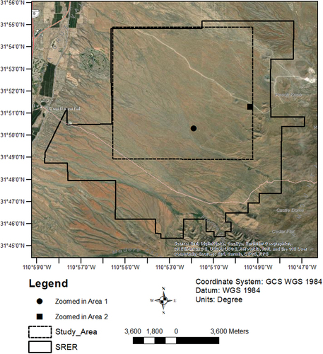
The Santa Rita Experimental Range (SRER) is a sparsely vegetated semi-arid mixed woody plant and herbaceous vegetation ecosystem in southern Arizona (Figure 1). This region experiences a bimodal growing season, with productivity dominated by monsoon rainfall in July and August and rainfall in winter and spring. Mean annual precipitation is 420 mm (2005–2014) and mean temperature is 17°C (2005–2014) (Biederman et al. 2017). The SRER has been an experimental site since 1902 and is the longest running continuous research facility with the aim of understanding rangeland ecosystems (Huang et al. 2018; McClaran 2003). Vegetation here is mostly a combination of woody mesquite trees with under-canopy and inter-canopy herbaceous plants such as perennial grasses and annual forbs and grasses (Biederman et al. 2017; Scott et al. 2015). The maximum canopy height is about 6 m to 15 m (Gallery 2014; Archer et al. 2017).

Figure 1. Study area within the Santa Rita Experimental Range (SRER) in SW Arizona. The solid line represents the entire SRER and the dashed line the selected study area based on vailability of ”good” data (see Section 2.2). The background image source: 0.5 m resolution WorldView-2 imagery collected in 2020.

2.2. Data

Since August 2017, the NEON AOP has collected airborne data annually using their very high resolution (1 m) hyperspectral imaging spectrometer, a discrete and full-waveform LiDAR instrument, and a high resolution digital camera (see Table A1 and Appendix A for more information on each dataset). In this study we used the NEON AOP data from August 2018 (Appendix A). All three types of data are taken at the same time of day and from the same height (1000 m). In the following subsections we describe the three NEON datasets in more detail plus an additional set of drone images taken 9 months after the NEON AOP data that were used for evaluating classification accuracy (Table 1).

Table 1. Data for classification and accuracy assessment.

Data Type	Description	NEON Data Product Name	Resolution	Date Range	Source/DOI	NEON Product ID
Hyper- spectral raster product	Atmospherically corrected 426 bands image from the NEON Imaging Spectrometer.	Spectrometer orthorectified surface directional reflectance – mosaic	1 m	Aug, 2018	NEON: https://doi.org/10.48443/qeae-3x15	DP3. 30,006.001
Canopy height †	This CHM product is created from LiDAR point clouds	Ecosystem structure	1 m	Aug, 2018	NEON: https://doi.org/10.48443/05q5-9352	DP3. 30,015.001
Digital camera imagery	Orthorectified level 3 RGB camera images	High resolution orthorectified camera imagery mosaic	0.10 m − 0.25 m	Aug, 2018	NEON: https://doi.org/10.48443/4e85-cr14	DP3. 30,010.001
Drone Imagery	Orthorectified RGB camera images	–	0.01 m	May, 2019	SRER ecostate mapping project: https://doi.org/10.25739/1w46-n223	–

†A reprocessed canopy height data was personally collected from NEON(see section 2.2.2.

2.2.1. Hyperspectral images

We used the NEON AOP level 3 (L3) orthorectified surface reflectance data product from August 2018 distributed in 1 km by 1 km tiles with a 1 m spatial resolution including all 426 bands from the NEON Imaging Spectrometer. Level 1 (L1) flight line radiance data collected by the NEON Imaging Spectrometer are first orthorectified and resampled into a uniform spatial grid using nearest neighbour resampling. Level 2 flight line reflectance and L3 surface directional reflectance tile data are then produced from the L1 at-sensor radiance product through atmospheric correction with Atmospheric & Topographic Correction (ATCOR) processing (Karpowicz and Kampe 2015). See Appendix A1 for more information on the hyperspectral imaging spectrometer and NEON data processing.

2.2.2. Canopy height model from LiDAR data

We used the NEON canopy height data – i.e. the height of the top of the canopy relative to bare ground – that were created from LiDAR point clouds collected in August 2018 (please see Appendix A2 for LiDAR instrument specifications and method for CHM generation). The publicly available NEON CHM data is created based on 2 m lowest height cut-off value, 5 m CHM height threshold interval, and 3 m CHM maximum interpolation distance (for further details see Appendix A2). At SRER, the woody plants are not very tall: the maximum CHM height in this study area is about 7.5 m (the maximum height elevation band). Thus, this standard 2 m NEON lowest height cut-off for CHM creation is not well-suited for desert sites such as SRER as it will not capture the woody plants with heights lower than 2 m. Thus, NEON reprocessed the CHM for our study with a lower height cut-off of 0.67 m and 1 m CHM interval (B. Hass, pers. comm.). As for the hyperspectral data, NEON provides the CHM data in 1 km by 1 km tiles with a spatial resolution of 1 m.

2.2.3. Digital camera imagery

We used the NEON AOP Level 3 (L3) orthorectified very high spatial resolution RGB camera imagery collected at the same time as the hyperspectral and LiDAR data in August 2018 (see Appendix A3 for camera instrument and data processing). The orthorectified and georeferenced camera images were provided in a 1 km by 1 km raster image format with a fixed spatial resolution of 0.1 m using nearest-neighbour resampling (W. Gallery, pers. comm.) (Gallery 2019).

2.2.4. Drone imagery

The drone images were collected in May 2019 (see Appendix A4 for camera instrument and data processing). The spatial resolution of the products was 1 cm ground sampling distance. This very high resolution orthomosaic camera image product has limited coverage (<1%) over the study area and were not collected at the same time as the NEON AOP data, so we only used this dataset to visually verify tall woody plant cover when creating the reference dataset (see Appendix B).

2.3. Data pre-processing

We performed several image pre-processing tasks (first column in Figure 2) before performing the classification, which are described in the following subsections.

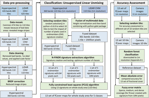
Figure 2. Flow diagram of the pre-processing, classification, and accuracy assessment methods. Note that “multimodal” data refers to the combination of hyperspectral and LiDAR-derived canopy height model (CHM) data (see Section 2.4.2).

2.3.1. Image mosaicing

All tiles from both the hyperspectral and LiDAR images had to be mosaiced into one complete dataset covering the entire study area. The LiDAR data tile coverage was greater than that of the hyperspectral data, despite the fact both instruments were flown on the same platform at the same time, due to the different instrument characteristics in collecting data (see Section 2.2). Furthermore, creating the mosaic for the hyperspectral data required some quality control checks that reduced the number of tiles. Out of 625 LiDAR-derived height data tiles, and 489 hyperspectral data tiles, we merged the 474 tiles common to both datasets to create an image mosaic that covers the entire SRER. However, in the southern and eastern part of SRER, both datasets had regions with missing data or dark areas with illumination problems due to the presence of clouds during image acquisition (Fig. S1). The final selected area was a rectangular box in the NW corner of the SRER that contained both ‘good’ and ‘moderate’ weather flight lines (See Appendix A1 and Fig. S1 and see NEON Spectrometer L1 reflectance and L2 product QA

information for SRER ATBD Section 4 for discussion of the quality control flags). The selection of this final study area removed all missing data and cloud cover shadows and finally contained 110 tiles.

2.3.2. Data cleaning

We removed all so-called ‘bad’ bands from the 426 band hyperspectral image. The bad bands are present mostly in the water vapour spectral range due to atmospheric corrections of water vapour absorption bands, gaseous absorption primarily due to the oxygen A-band absorption band and a strong carbon dioxide band (Karpowicz and Kampe 2015). Therefore, we removed the bad bands using the bad band spectrum range provided in metadata information contained in each NEON HDF5 file. After removing the bad bands we had 360 clean bands. We also removed ‘no data’ values and applied the scale factor provided in metadata information.

Within our study area, we found erroneous maximum CHM height values due to the presence of a power line, which reached about 22 m. Therefore, we converted the CHM height over 9 m to 0, as the maximum woody plant height within the study area is about 9 m.

2.3.3. BRDF correction

The L3 surface hyperspectral reflectance data (see Section 2.2.1) do not account for Bidirectional Reflectance Distribution Function (BRDF) effects, which are differences in reflectance due to the viewing and illumination geometry (Colgan et al. 2012). When the hyperspectral image tiles were mosaicked together, we found that our final study area had some artificial vertical stripes, or ‘seamlines’, that come from stitching the flight paths from the push-broom sensor and related BRDF effects (Fig. S2a). To address BRDF effects, we corrected the L3 surface reflectance to nadir using a BRDF model (see Section 2.3.3). For the BRDF correction, we used a kernel-driven Li-Ross model (Wanner, Li and Strahler 1995; Colgan et al. 2012). The Li geometric scattering kernel and the Ross volumetric scattering kernel were calculated using the equations from Wanner, Li and Strahler (1995) and following the similar method described in Colgan et al. (2012). The BRDF correction scripts were adapted from those used in (Marconi et al. 2021) and applied to our data (see Data, Code, and Software Availability section). We applied all four combinations of Li-sparse versus dense geometric scattering kernels and the Ross-thin versus thick volumetric scattering kernels on a single tile. The change in Li-sparse/dense combination had more impact on BRDF correction compared to the change in the Ross-thin/thick combination. Although our study area has sparse woody plants, similar to Colgan et al. (2012) we found the best BRDF correction using Li-dense.

The BRDF correction removed the vertical seamlines present in the study area (Fig. S2b). However, in addition to the vertical seamlines, there was also a non-straight line present in the middle of the study area due to the NEON’s method for selecting pixels based on the Weather Quality Index (Appendix A1). For selecting pixels to create the L3 mosaic, NEON gives first priority to the best weather pixels and then second priority to the pixels closest to nadir. The non-straight line present in the middle of the study area is most probably the intersection of two days with differing weather conditions (T. Goulden pers. comm.). Therefore, this line presents where the highest quality weather pixels meet the lower quality ones. The BRDF correction mostly removed this additional non-straight seamline, but some portions of it are still visible in the resulting image (Fig. S2).

2.4. Classification methodology

2.4.1. Unsupervised linear unmixing of hyperspectral data

We chose unsupervised linear unmixing (commonly referred to as ‘spectral unmixing’ when using multispectral or hyperspectral remote sensing data – see Introduction) to estimate fractional coverage of all the main cover types (tall woody plants with a defined canopy, herbaceous vegetation, and bare soil) in our study area. The analysis process has two steps: the first step extracts signatures for each endmember (i.e. each cover type class) and the second step calculates the abundance of that specific class in each pixel.

After testing different endmember extraction algorithms (Appendix C), we chose the N-FINDR algorithm to extract endmember signatures. Then, the final fractional cover map is created based on the estimation of different proportions of endmembers in the pixels. The most popular inversion method for finding the optimal fractional cover of each end member is the least squares algorithm. We used the fully constrained least squares (FCLS) algorithm because it constrains sum-to-one the fractional cover of all endmembers in a pixel.

2.4.2. Fusion of LiDAR-derived canopy height and hyperspectral data in the unsupervised linear unmixing algorithm

After applying the unsupervised linear unmixing approach on hyperspectral data only, we then applied it to the fusion of both hyperspectral and LiDAR-derived CHM data (Table 1). The height information in the LiDAR-derived CHM product was read in and added to the 360 band hyperspectral data to create an extra band or dimension of data (i.e. 361 dimensions) before the linear unmixing classification was performed (Figure 2). The hyperspectral image band values are normalized surface reflectances that range from 0 to 1. The height data ranges from 0 to 9 m in metres. Therefore, we normalized the height data to their maximum and minimum heights over the entire study area using the following equation:

(1) $\overline{h_i}=\frac{h_i-min\left(h_a\right)}{max\left(h_a\right)-min\left(h_a\right)}$(1)

where h_i is the raw CHM height for pixel i, max(h_a) and min(h_a) are the maximum and minimum height of the raw CHM over the entire tile area, and $\overline{h_i}$ is the normalized height for pixel i.

We modified the following equation from the original N-FINDER algorithm (Winter 1999) to apply it on the fused hyperspectral and height data:

(2) ${\mathrm{d}}_{\mathrm{i}\mathrm{j}}=\sum _{\mathrm{k}}\left(e_{\mathrm{i}\mathrm{k}}\right){\mathrm{c}}_{\mathrm{k}\mathrm{j}}+\epsilon$(2)

Where, $d_{ij}$ is reflectance or height data for the ith band of the jth pixel, $e_{ik}$ is reflectance or height for the ith band of the kth endmember, $c_{kj}$ is the fCover for the jth pixel from the k-th endmember, and $\epsilon$ is gaussian random error (assumed to be small). The fused dataset is an augmented vector (d) combining hyperspectral reflectance ($\rho$) and height data (h): d= [$\rho$₀, …, $\rho$_i-1, h_i]. Our expectation is $h_k$ = 0 for herbaceous vegetation and bare soil or biocrust. $h_k$ >0 for woody cover and $h_k$ is higher for large woody plants compared to smaller ones. The N-FINDR algorithm therefore created endmember signatures using both the spectral and height data, and FCLS algorithm (Winter 1999) calculated the fractional cover of each of the spectral endmembers for each pixel.

2.4.3. Endmember testing

In a preliminary analysis using only one tile, we tested using two to seven endmembers in the N-FINDER endmember extraction analysis to assess which number of endmembers is best for obtaining the fractional cover of the main cover types we wish to identify in the study area. Although we sought to separately identify three main cover types, three endmembers was not enough to account for the presence of shadows from tall woody plant canopies onto bare ground. Increasing the number of endmembers to six and seven primarily resulted in separating the non photosynthetically active vegetation cover types into more classes. In the end, the number of endmembers was a compromise between not getting the correct vegetation classes and also not having too many ‘bare soil’ or ‘other’ classes that are not well represented in the spectral libraries. Therefore, in our final classification analysis, we focused on testing the differences between using four or five endmembers over different regions of the study area (see Results Section 3.1), and both with and without canopy height information included (see Results Section 3.2).

2.4.4. Testing random tile (number of pixels) selection for endmember signature generation

Due to computational cost constraints related to the large size of the data involved, we could not use all the 110 1 km × 1 km image tiles that cover the entire study area in the endmember signature generation. Instead, we found that using a maximum of 10 image tiles in the endmember selection resulted in a tradeoff between using as much of the data as possible and the computational time taken for the endmember generation algorithm to run. The 10 image tiles used in the endmember selection covered about 9.1% of the entire study area. These 10 tiles were randomly chosen and were checked for data gaps: Only tiles with no data gaps were used for endmember selection. For the random selection of image tiles included in the analysis, we used the random.sample() function in python v3.6.8 for selecting multiple random items without replacement and we added a seed function so that the same random tiles are selected for each testing. Each tile contained one million pixels. To evaluate the impact of using fewer tiles on the endmember generation, we tested how the classification accuracy changed when using endmember signatures extracted from an increasing number of image tiles selected from these randomly selected 10 tiles. First, endmember signatures were created from each of the randomly selected image tiles (resulting in 10 different sets of endmember signatures), then two sets of five randomly selected tiles were used for endmember signature generation (resulting in an additional 2 sets of endmember signatures), and finally, all randomly selected ten tiles were used to derive the endmember signatures (resulting in 1 final set of endmember signatures). These tests therefore resulted in 13 sets of endmember signatures that were used to create the fCover maps for the entire study area. We compared the simple mean absolute error metric (see Section 2.5.2) between these 13 fCover maps and the reference map (see Section 2.5.1) to determine if increasing the number of image tiles used in the endmember signature extraction resulted in an improvement in classification accuracy. These results are described in Section 3.3.

2.5. Accuracy assessment

2.5.1. Generating the reference dataset

We needed a reference dataset to assess the accuracy of our unsupervised mixed pixel (spectral unmixing) classification of the 1 m resolution hyperspectral and LiDAR data. For this purpose, we performed a supervised pure pixel classification of the 0.1 m resolution 10 randomly selected camera images using a random forest (RF) model and then aggregated to 1 m resolution to obtain the fractional cover of the main cover types for validating the 1 m unsupervised classification of the hyperspectral and LiDAR-derived height data (please see Appendix B for the details of creating reference dataset and its accuracy assessment).

2.5.2. Accuracy assessment methods and application

Compared to discrete (e.g. pure pixel) classifications, it is more difficult to perform an accuracy assessment for classifications of continuous variables such as vegetation and soil fractional cover, especially in spatially heterogeneous mixed woody plant-herbaceous semi-arid ecosystems. The actual fractional cover is hard to determine precisely, even with ground truth data collected in situ, and therefore errors in the reference data used for accuracy assessment are likely to be high (Congalton and Green 2019). For the accuracy assessment of the 1 m fCover maps, we used a supervised classification of the higher resolution 0.1 m camera images as a reference map (see section 2.5.1) and aggregated the 0.1 m classified camera images to 1 m resolution to get the fractional cover of each class at the scale of the classified fCover maps. We then compared the fraction of each class from our reference dataset with the fraction of each corresponding class in our fCover maps using the so-called ‘fuzzy error matrix’ method, which is designed for continuous classifications and is therefore more appropriate than the traditional error (or confusion) matrix approach (Congalton and Green 2019). In the fuzzy error matrix approach, the classified fractional cover is labelled as ‘acceptable’ if it is within a user-defined percentage fractional cover of the actual reference fractional range class (Congalton and Green 2019, 60–164). The ‘acceptable’ fractional covers are therefore included as an accurately classified class.

For the construction of the fuzzy error matrix of a continuous variable, fractional cover ranges are defined based on knowledge of the spatial distributions of the cover types in the study area (instead of comparing each percentage cover). For our accuracy assessment of the SRER fCover maps we wanted to capture the fractional coverage detection accuracies for very low or sparse cover, medium cover, and dense coverage of each class (e.g. the different vegetation or soil cover types). Therefore, we defined three class cover ranges for the fuzzy error matrix calculation: 0–30%, 30–60%, and 60–100% fractional cover. Then, we defined an acceptable range if the classified fractional cover is within the 10% of the reference dataset. We constructed three error matrices for the three main classes: tall woody plants, herbaceous and low stature vegetation, and bare soil fractional coverage. Then, we used these three fuzzy error matrices to calculate both the overall accuracy ands the errors of commission and omission for each fractional cover range of each class (see results in Section 3.4 and Table 2). Given the more complex error calculations involved in the fuzzy error matrix method, we have only described fuzzy error matrix accuracy assessment for the SRER fCover map derived using all 10 randomly selected tiles for endmember signature generation (see Section 2.4.4). For example, in our case with the three fractional cover ranges that we have defined, for woody plants an error of commission for the 0–30% fractional cover range would occur if higher fractional ranges of woody plant cover (outside the additional 10% ‘acceptable’ window) are classified as 0–30% woody cover or if other cover types are erroneously classified as 0–30% woody plant cover. An error of omission would occur if 0–30% range woody cover is classified in a different higher fractional cover range (>40% coverage) or as other cover types.

Table 2. Errors of omission and commission for different class coverage.

		Fractional Cover Range (%)
Class	Error (%)	0-30	30-60	60-100
Tall woody plants	Omission	2.8	64.2	98.1
	Commission	24.5	68.6	44.7
Herbaceous	Omission	9.7	71.3	99.9
	Commission	59.9	71.9	94.7
Other	Omission	54.8	29.5	5.2
	Commission	0.3	73.9	34.5

Note: For each class cover types rows are presenting errors of commissions and Omissions. Columns are presenting the errors for different fractional cover groups representing sparse (0–30), medium (30–60), and dense (60–100) class covers (sample size 10,000,000).

Given the fuzzy error matrix method does not provide one simple metric with which we can evaluate the fCover maps, we also compared the fractional cover for each class and for each of the 13 classifications (Section 2.4.4) to the reference dataset using the following mean absolute error (MAE) equation (Colditz 2015):.

(3) $MAD=\frac{1}{N}\left({\sum }_{n=1}^N\left|M_n-R_n\right|\right)$(3)

where N is the total number of pixels covering all reference tiles (10,000,000 pixels), and M_n and R_n are the fractional cover for each pixel n in the classified and reference dataset, respectively. The MAE is used to evaluate the impact of including a different number of tiles in the endmember signature generation (see methods Section 2.4.4 and results described in Section 3.3). In Section 3.4 we compare the results from the fuzzy error matrix and MAE accuracy assessments. We note that while both accuracy metrics refer to ‘error’, we consider that these methods refer more to the difference between the classification and reference datasets, given the fact that the reference dataset also contains errors of omission and commission (the reference dataset accuracy assessment is presented in Appendix B3).

All data analyses were conducted with Python v3.6.8 (see Data, Code, and Software Availability Statement). We used the Python PySptools package (v0.15.0) to perform all steps of the spectral unmixing, and the H5py package and the Python GDAL v3.3.2 library to read and preprocess the images.

3. Results

3.1. Linear unmixing of hyperspectral images using different numbers of endmembers

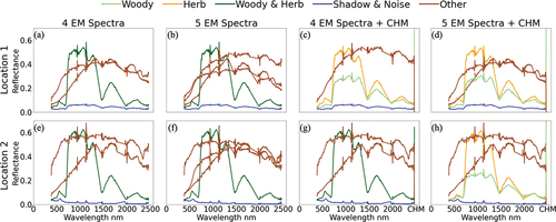
First, we tested whether we could separately detect two distinct vegetation signatures with unsupervised linear unmixing of hyperspectral data only using different numbers of endmembers. The first two columns of Figure 3 show the spectral signatures derived when specifying 4 endmembers (EM) and 5EM in the signature extraction algorithm, respectively. In both the 4 and 5EM unmixing using only hyperspectral data, the linear unmixing derived only one clear vegetation signature (green ‘Woody & Herb’ curves in Figures 2 (a), (b), (e) and (f)). This signature therefore captured all the PV cover: there was no separation of the tall woody plants versus herbaceous vegetation. All other signatures for endmember selection based on hyperspectral data alone were either shadow and noise (blue curves), or different soil or non-vegetation spectra (brown curves labelled as ‘other’ in Figure 3). Increasing the number of endmembers from 4 to 5 only resulted in a greater number of the ‘other’ classes (two for 4EM, and three for 5EM). The ‘other’ classes are likely different types of NPV cover that could include bare soil, dry senesced grasses, and/or biological soil crusts (biocrusts). There are generally two distinct spectra that we have labelled as ‘other’ NPV classes: The signatures with generally high reflectance across the hyperspectral range (e.g. Figure 3 (e)) could be bare soil. The signatures with a much shallower increase in reflectance in the visible and near infrared, with two peaks around 1300 and 1700 nm and a small decrease in reflectance due to water absorption around 1400 nm, could be biocrusts (cf. fig.10 in Smith et al. 2019). We discuss possibilities for what these ‘other’’ endmember signatures could represent further in Section 4.2. However, our main goal of separating woody plants versus herbaceous vegetation was not achievable when only hyperspectral data was used in the classification.

Figure 3. Spectral responses of four versus five spectral endmembers (EM) with and without LiDAR derived canopy height model (CHM) data in two different cases, where tall woody plants and herbaceous cover were separated based on different combinations of data and EM numbers. The first two columns are the spectral signatures with 4EM and 5EM in the unsupervised linear unmixing algorithm on hyperspectral data only, and last two columns are the spectral signatures with 4EM and 5EM in the unsupervised linear unmixing algorithm on hyperspectral with height data. Zoomed in area 1 (a-d): case where tall woody plants and herbaceous cover were separated only by using both four and five endmembers with the fusion of hyperspectral and height data. Zoomed in area 2 (e-h): case where tall woody plants and herbaceous cover were separated only by using five endmembers with the fusion of hyperspectral and height data.

3.2. Benefit of including canopy height with hyperspectral data in the linear unmixing procedure

Second, we tested whether we could separately detect two distinct vegetation signatures when combining both hyperspectral and LiDAR canopy height data in the unsupervised multimodal unmixing procedure. As for the classification analysis described in Section 3.1, we also tested using 4 versus 5 endmembers in the endmember signature creation. For some locations (individual image tiles) we were able to separately detect two vegetation signatures when canopy height data were included with the hyperspectral data in the signature creation with only 4 endmembers (e.g. compare the light green ‘Woody’ curve with the orange ‘Herb’ curves in Figure 3(c)). However, for other locations we needed 5EMto achieve the separation of the two vegetation classes (Figure 3(h)). These results therefore show that whether or not inclusion of LiDAR-derived canopy height data helps to distinguish two vegetation signatures in the endmember signature creation depends on the number of endmembers included in the linear unmixing analysis. Two vegetation signatures are detected when including hyperspectral and height data in the unmixing analysis, but only when 5EM are specified. This is true for most of the 10 individual randomly chosen image tiles when they are used in the signature creation, and when we used combinations of two different sets of 5 tiles or all 10 tiles in the signature creation (results not shown). Therefore, the optimum configuration for separating out two vegetation spectra using unsupervised linear unmixing for the SRER savanna site is when both hyperspectral and canopy height data are included in the unmixing algorithm with 5 endmembers (5EM+height).

Figure 4 and 5 present the fCover maps, camera and drone images, and the canopy height model (CHM) for the zoomed-in areas 1 and 2 corresponding to the top and bottom rows in Figure 3, respectively (see Figure 1 For the locations of the zoomed-in areas and Fig. S3 and S4 for fCover maps of all the endmember spectra shown in Figure 3). These two figures demonstrate that the unmixing algorithm does in fact identify the tall woody plants versus other photosynthetically active herbaceous vegetation when CHM data are included (cf. the Woody plant fCover maps and the CHM in both Figures 4 and 5) Figure 4 shows an example location for the first rarer case corresponding to the top row of Figure 2 in which two vegetation spectra were identified with 4EM+height, and Figure 5 shows an example location for the second more common case corresponding to the second row of Figure 2, in which 5EM + height was needed to separately detect two vegetation spectra. Comparing the location of CHM positive values and the woody plant fractions, the woody plant detection is dominated by CHM (Figure 4 (f), (i) and 5(h)). However, It is also possible that tall woody plants are accurately detected even when they are not apparent in the CHM (Figures 4 (f) and (i)). Furthermore, the presence of inaccurate positive CHM values that are clearly patches of bare ground or herbaceous cover were not detected as woody cover (see larger dark grey patches in the CHM map in Figure 5(c) versus the more ‘patchy’ low fractional cover woody plant patches in the woody plant fCover map in Figure 5(h)). However, as the CHM has a height threshold of 0.67 m (see section 2.2.2 and Appendix A2 for CHM data processing and height threshold), it is likely that woody plants smaller than 0.67 m may not be detected correctly. Instead of the reprocessed 0.67 m threshold, if we used the NEON provided CHM directly from their data download website we would have omitted more smaller woody plants. Therefore, the height threshold of the CHM is very important in separating woody plants versus other vegetation using this fusion method. However, although the fCover of woody plants is clearly dominated by CHM information, we reemphasize that it does not always help to separately detect those woody plants, especially when the optimum number of endmembers are not selected (e.g. for this site, see Figure 5).

Figure 4. Fractional cover with and without canopy height model using four versus five spectral endmembers (EM) in a “zoomed in” area (20 m x 20 m) (location: Figure 1 Zoomed in Area 1 corresponding to the top row of endmember signatures in Figure 3). In this location, both 4EM and 5EM unmixing based on the fusion of hyperspectral plus height data were able to separate tall woody plants (f and i) from herbaceous vegetation (e and h), although this was not common throughout the study area. a) 0.1 m resolution camera image collected at the same time (August 2018) on the same NEON AOP flight as the hyperspectral and LiDAR data, b) 0.01 m resolution drone image at this location collected in May 2019, and c) 1 m resolution canopy height data derived from LiDAR data. d) and g) the vegetation fractional cover maps for 4 EM and 5 EM based on including hyperspectral data only in the linear unmixing classification. e), f), h) and i) the vegetation fractional cover for the 4 EM and 5 EM based on the fusion of hyperspectral plus LiDAR-derived height data from the CHM.

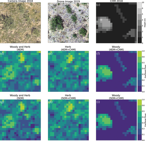
Figure 5. Fractional cover with and without canopy height model using four versus five spectral endmembers (EM) in a “zoomed in” area (30 m x 30 m) (location: Figure 1 zoomed in Area 2 corresponding to the bottom row of endmember signatures in Figure 3). In this location, only the unmixing with 5 EMbased on the fusion of hyperspectral plus height data was able to separate tall woody plants (h) from herbaceous vegetation (g), which was the case for most of the study area. a) 0.1 m resolution camera image collected at the same time (August 2018) on the same NEON AOP flight as the hyperspectral and LiDAR data, b) 0.01 m resolution drone image at this location collected in May 2019, and c) 1 m resolution canopy height data derived from LiDAR data. d) and f) the vegetation fractional cover maps for 4 EM and 5 EM based on including hyperspectral data only in the linear spectral unmixing classification. e), g) and h) the vegetation fractional cover for the 4 EM and 5 EM based on the fusion of hyperspectral plus LiDAR -derived height data from the CHM.

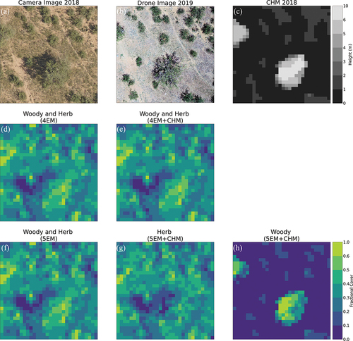
When examining the Woody fCover maps (Figure 4 (f), (i)and 5(h)) more closely we can see that the larger denser woody plant patches (e.g. with larger crown areas) have high fractional coverage (e.g. light yellow patches to the centre left of Figure 4 (f) and 4(i) or the bottom centre of Figure 5(h)) and individual or smaller patches of woody plants typically have very low fractional coverage (e.g. bottom right of Figures 4 (f) and (i) and top right of Figure 4 (h)). This visual inspection indicates that large patches of woody plant coverage are detected with higher accuracies compared to smaller woody plant patches. Even at 1 m spatial resolution and with woody plants captured by the CHM, using both hyperspectral and height data with a mixed pixel method did not result in 100% coverage for clearly defined woody plant patches (see the camera images in Figures 4 and 5 for a visual comparison): The unmixing algorithm was still able to detect other cover type fractions within woody plant canopies.Partly this was due to reflection of light from the ground and other canopy elements in-between the woody plant branches or shadows. Smaller patches of individual woody plants have an even lower percentage crown cover compared to dense woody plants with large crowns; therefore, even herbaceous vegetation or bare soil will be detected as understorey of these smaller woody plant patches. Even when a large woody plant occupies a whole pixel (see camera and drone images in Figures 4 and 5), having fewer leaves in the canopy accompanied by ground reflection through the leaves and the presence of shadow within the canopy may result in a low woody plant fractional cover, potentially resulting in errors of omission when comparing with the supervised reference dataset (see Section 3.4). The herbaceous fractional cover detected by this mixed pixel classification method was able to capture both the open herbaceous vegetation (between the woody plant patches) and under canopy herbaceous cover (Figure 4 (e), (h) and 5(g)). The fractional herbaceous cover is much lower under large woody plants than for smaller woody plants.

We can conclude that including height data from the LiDAR CHM in the linear unmixing with hyperspectral data helped to separate out the tall woody plants versus herbaceous vegetation, with the caveat that smaller shrubs below the height threshold used to derive the CHM will not be included in our ‘woody’ plant class. Without height data, all vegetation is typically detected in a single mixed woody and herbaceous PV vegetation class (Figures 4 (d), (g), 5(d) and (f)). Our analysis of zoomed-in areas presented in Figures 4 and 5 further showed that using 5EM is preferable to 4 for the endmember signature creation. Therefore, for the classification accuracy assessments and whole study area fCover map creation, we selected five endmembers that represent: (1) tall woody plants (>0.67 m) with a clear vertically structured canopy, (2) low stature shrubs and non-woody herbaceous vegetation, (3) a non-PV ‘other’ class that likely to be bare soil, (4) another non-PV ‘other’ class that likely consists of biocrusts or dry grasses, and (5) canopy shadows.

3.3. Mean absolute error metric to test the number of pixels (tiles) included in signature extraction

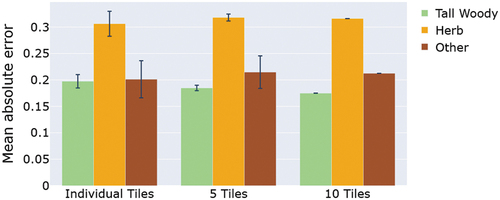
As discussed in Section 2.5, assessing the accuracy of fractional cover maps classified using mixed pixel methods is more complex than comparing single classes assigned to each pixel using pure pixel classification methods. The mean absolute error (MAE - Section 2.5.2) was calculated between each of the 13 sets of classified fractional cover maps (Section 2.4.4) and the 1 m aggregated reference dataset to test if the fCover accuracy for each class varied with the number of pixels (image tiles) included in the classifications. Because we are using 5 EM in our unsupervised linear unmixing classification, and not 4, we had an extra class in the 13 set of classified maps that we could not directly compare with the reference image because that additional class was not included in the supervised classification of the reference dataset (see Section 2.5.1). Therefore, we kept the tall woody plant and herbaceous classes and combined all other classes as other’ for the accuracy assessment (here and in Section 3.4).

A MAE of 0.2 means that there is on average an absolute fractional cover difference of 0.2 between the classified and reference datasets. Figure 6 shows the mean and standard deviation of the MAE between the classified and reference maps across the 10 sets of classifications from endmembers extracted from each of 10 individual tiles (left set of barplots), the mean and standard deviation of the MAE across the two sets of classifications using 5 tiles used in endmember selection (middle set of barplots), and finally the MAE for the classification when all 10 randomly chosen tiles were included in the endmember signature creation (right set of barplots in Figure 6). As Figure 6 shows, the number of tiles for endmember extraction did not drastically affect the classification (MAE) accuracy of any of the three main classes (woody plants, herbaceous, and other non-PV cover types). The mean MAE slightly decreased for tall woody plant fCover detection with an increasing number of tiles used in the endmember signature extraction. For the herbaceous and ‘other’ class (encompassing bare soils, dry grasses, and biocrusts) the fCover detection accuracy varied slightly depending on the number of tiles used for EM extraction.

Figure 6. Comparison of the mean absolute error (MAE) between the classified and references maps for the 13 sets of classifications derived using a different number of image tiles (or number of pixels) included in the endmember signature extraction (see Section 2.4.4). (10 sets of signatures extracted from individual tiles, two sets of signatures extracted from five tiles, and one set of signatures extracted from ten tiles). The bars represent the mean MAE and the error bars give the standard deviation for each endmembers fCover sets based on numbers of tiles included in signature extraction. For example, the left set of bar plots represents the mean and standard deviation in MAE across all 10 classifications based on 10 different sets of endmember signatures generated from all 10 individual randomly selected tiles.

3.4. Comparing the classification accuracy for each cover type based on the fuzzy error matrix approach and MAE

In a second accuracy assessment step, we calculated the overall accuracy and errors of commission and omission of our three main classes using the fuzzy error matrix approach of Congalton and Green (2019 - Section 2.5.2) to test in more detail if classification accuracy is similar for all cover types. For the sake of simplicity, and as the fCover accuracy did not vary drastically with varying the number of pixels (image tiles) included in the classifications (Section 3.3), in this section we only assessed the accuracy of the classification that used all 10 randomly selected image tiles together in the endmember signature extraction. As in Section 3.3, fuzzy error matrices were created for three main cover classes: tall woody plants, herbaceous vegetation, and a non-PV ‘other’ cover type class that potentially represents a mix of bare soil, dry grasses, and biocrusts. The overall accuracies for tall woody plants, herbaceous vegetation, and the ‘other’’class based on the fuzzy error matrix approach were 71%, 39%, and 56%, respectively. The higher accuracy for the tall woody plants was comparable to the MAE analysis. The herbaceous cover detection accuracy was generally lower than for the tall woody plants and ‘other’ class, again similar to the MAE analysis. Both the fuzzy error and MAE values represented uncertainties in both the classified maps and the reference dataset. For example, the higher overall error from the fuzzy matrix approach or MAE for herbaceous is likely partially related to the fact that the errors of omission for the reference herbaceous fractional cover were higher than errors of omission or commission for the other cover types (Appendix B3).

The three class fractional cover ranges that we have defined for the fuzzy error matrix calculation (0–30%, 30–60%, and 60–100%) are considered to capture very low or sparse cover (for each class), medium coverage, and dense coverage, respectively. For tall woody plants, the sparse density woody plants (0–30%) have the lowest errors compared to the high density coverage (60–100%), especially for errors of omission (Table 2). This is in line with our visual analysis in Section 3.2, which indicated that dense woody plant canopies may not have 100% fractional cover because a mixed pixel classification detects reflectance from between canopy elements as well as canopy shadows. However, it is also possible that the underestimation of high density woody plant cover in the classified maps is just relative to the overestimation of tall woody plants in the reference dataset (Appendix B3).

Herbaceous fractional cover detection is generally less accurate compared to tall woody plant fractional cover detection (higher errors of omission and commission for the herbaceous class in Table 2 across all fractional cover ranges), as was the case for the MAE analysis. The classification is not able to capture medium or high fractional cover of herbaceous vegetation compared to the reference image, with high percentage errors of commission and omission. This high uncertainty is likely because smaller woody plants are being included as herbaceous in the classification, whereas they are classified as woody plants in the reference dataset (Appendix B3). Furthermore, dry grasses may have been classified as herbaceous vegetation in the reference dataset, but ‘other’ in the unsupervised mixed pixel classified fCover maps.

For pixels where the fCover of the non-PV ‘other’ class is low (i.e. where the ground is mostly covered either by dense herbaceous or woody vegetation – the 0–30% fractional cover range), the error of commission is very low compared to error of omission which indicates an underestimation of the sparse cover of ‘other’ class (Table 2 bottom two rows). It could mean that pixels that should be classified as low fractional cover for the non-PV ‘other’ class are being classified as herbaceous vegetation. This might explain the high errors of commission for the herbaceous class.

For the estimation of mid-range fractional coverage of all classes, the errors of commission and omission are much higher than other low and high fractional class cover detection. This indicates that ‘medium density’ cover fractions of any type are typically harder to detect, even with the relatively broad fractional cover ranges that we have defined here.

3.5. Whole study area classification: description and comparison to previous fcover studies at SRER

In this section, we present the classification of the whole SRER study area using the 5 EM signatures derived using both hyperspectral and LiDAR-derived CHM data and all 10 randomly selected image tiles in the endmember signature extraction. Figure 7 shows fCover maps for the whole study area for: a) tall woody plants, b) herbaceous vegetation, and c) the non-PV ‘other’ class that combines bare soil and other NPV signatures. Note that we are not presenting the shadow fractional cover map because our objective was not to detect shadows – we only included a ‘shadow’ class in the unmixing procedure to ensure that canopy shadows were not included in other classes.

Figure 7. Fractional cover maps for the whole SRER study area (dotted line in Figure 1) for the three main cover types: a) tall woody plant fCover; b) herbaceous vegetation fCover; and c) fCover of all other non-PV classes combined together (likely consisting of a mix bare ground, biocrusts and dry grasses). fCover maps were derived using the unsupervised linear unmixing on fusion of hyperspectral and LiDAR -derived canopy height data. The flight seam that we could not remove completely with BRDF correction is slightly visible in the ‘other’ class fCover map.

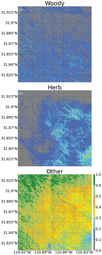
Tall woody plants have higher density coverage in the SE region of the study area where the elevation increases (Figure 7(a)). The high fCover areas of tall woody plants in the western and northern regions of the study area tend to follow specific spatial patterns. These woody plant patterns are following water drainage lines or ‘washes’ where there is easier root water access. Herbaceous vegetation also exhibits higher density in the SE region of the study area (Figure 7(b)), and much lower fractional cover in the northern and western part of the study area, in contrast to the ‘other class, which has the highest density cover in those areas (Figure 7(c)). This contrast in spatial patterns between the photosynthetically active herbaceous vegetation class and the ‘other’ class comprising bare soil and other NPV types is likely driven by elevation and precipitation gradients, which are higher in the southeast and decline towards the northwest (McClaran 2003).

Finally, we visually compared our results with two existing shrub fCover products covering the SRER. We provided a qualitative, instead of quantitative, comparison because those products were derived at different temporal and spatial scales. These two products are the mean (1984–2011) woody cover (at 30 m resolution derived from Landsat Thematic Mapper [TM] images - Huang et al. 2018) and the National Land Cover Database Shrubland dataset from the USGS (“National Land Cover Database (NLCD) 2016 Shrubland Fractional Components for the Western U.S. (ver. 3.0, July 2020)” 2020) (Yang et al. 2018). Huang et al. (2018) used the automated Monte Carlo unmixing (AutoMCU) technique (Asner and Lobell 2000), which is typically used to separate PV from NPV classes. As their focus was woody plant detection they specified that the PV class consisted of only woody plants and categorized that all other classes as NPV. They found underestimation of woody cover on undisturbed areas and overestimation on disturbed areas (Huang et al. 2018, 2007). After a visual inspection of these two products and our product, we found that our woody plant fCover map is more similar to the NLCD shrub fCover product compared to the mean shrub map produced by Huang et al. (2018). At 30 m resolution, NLDC data did not capture the spatial patterns of the shrubs that follow the drainage lines or ‘washes’, which are present in our map. The mean woody cover map (Huang et al. 2018) did capture the shrubs near washlines even at 30 m resolution but it appears that they estimated a much higher mean shrub fCover compared to the NLCD data and the results presented in this study. The higher shrub fCover estimates derived in Huang et al. (2018) are likely due to the fact that they categorized all PV cover as woody plants and did not attempt to separate out the different PV types into separate vegetation cover classes, as we have done in this study.

4. Discussion

4.1. Challenges of accuracy assessment for classified fractional cover estimates in spatially heterogeneous mixed woody plant-herbaceous vegetation ecosystems

Deriving a reference fractional cover dataset to use for validation is challenging, as we discussed in Sections 2.5.2 and 2.5.4. In past fractional cover classification studies validation data used for accuracy assessment have either been collected from field-based ground truthing (Dashti et al. 2019; Swatantran et al. 2011) or derived from other fractional cover classifications (Colditz 2015). However, as we discussed in the methods, even ground truthing data could have errors related to difficulties of measuring the fractional cover of a specific class within a specific area (even for 1 m pixels) (Congalton and Green 2019), and this is likely to be particularly true in mixed woody plant-herbaceous vegetation ecosystems. Similarly, any other classified dataset that is used as a reference data is also likely to have classification uncertainties associated with it. The aforementioned past studies have typically considered the reference dataset as ‘truth’. In our study, we calculated the uncertainties in the pure pixel classification of the 0.1 m resolution camera images that we used as a reference dataset and attempted to take these uncertainties into consideration when comparing the classified maps to the reference data. Still, it is difficult to know how much errors of commission or omission in the classified datasets are propagated from uncertainties in the reference dataset, as we discussed in Section 3.4. What our accuracy analysis does allow us to conclude with some confidence are the following: i) areas with high density woody plant cover may have a lower fractional cover in the classified images because linear unmixing also detects between canopy elements and shadows (in that sense, the fractional cover is more comparable to plant area index than crown fractional cover); ii) accurate estimation of herbaceous vegetation is more difficult to achieve than woody plants or bare soil/NPV classes due to the fact that smaller shrubs may be included in this class, and dry grasses may be included in the non-PV ‘other’ class; and iii) detection of very mixed pixels (in which the fractional cover of different cover types within the pixel is in a medium range (e.g. 30–60%) is likely to have lower accuracy compared to low or high density fractional cover of any of the classes.

4.2. The case of the ‘other’ class

The fractional cover of the whole SRER study area was based on 5 EM that therefore produced five fCover maps: tall woody plants, herbaceous vegetation, shadow, and two maps derived using the two ‘other’ signatures that we consider to be either bare soil or another NPV cover type. This ‘other’ class has a high fractional cover over the whole study area (see Figure 7(c)). The low accuracy of the herbaceous class from both the MAE and the fuzzy error matrix accuracy assessments suggests that the ‘other’ class may include dry grasses. To test this, we re-categorized the two main different types of endmember signatures that were originally categorized as the ‘other’ class., We included all the NPV endmembers that had a gradual increase in reflectance, which we assume are either dry grasses or biocrusts (see Section 3.1), in the herbaceous class instead of the ‘other’ class, leaving all remaining NPV signatures that were originally categorized as ‘other’ as a separate ‘bare soil’ class (i.e. those signatures with generally high reflectance values across the hyperspectral reflectance range – see Section 3.1). Then we re-calculated the MAE between the classified and reference maps for the herbaceous and new ‘bare soil’ classes. This resulted in a much improved accuracy (lower MAE) for the herbaceous class (pink bars in Fig. S5), and an improved accuracy for the bare soil class (purple bars in Fig. S5). This analysis suggests that we have correctly identified the bare soil spectra, and that the other NPV spectra may indeed represent a type of ‘non-active’ (or senesced) dry grass.

However, the spatial distribution of herbaceous fractional cover drops considerably in the north and west of the study area (Figure 7(b)), which can be explained by the lower elevation and precipitation. In contrast, the fractional cover of the ‘other’ class dramatically increases in these regions. This suggests that it is unlikely that the ‘other’ class represents a dry grass cover type. Furthermore, the NEON data were collected in the middle of the monsoon period (data collected on August 24th, 27th, 28th, and 29th 2018) when plentiful rainfall would have resulted in increased vegetation activity since July across the entire SRER study area. Therefore, if the ‘other’ class does represent a type of grass or any other vascular plant species, the grasses would likely have been active and we would have detected a photosynthetically active vegetation spectral signature for all herbaceous vegetation.

Another alternative is that the ‘other’ NPV spectral endmembers with a more gradual increase in reflectance represent varying densities of biocrusts that are not easily discernible in the reference images, or even to an observer in the field. A comparison of these NPV signatures (Figure 3) with in situ hyperspectral signatures of different assemblages of both wet and dry biocrusts collected from a site in Utah (Smith et al. 2019 Fig.10) suggests that these spectral signatures with a more gradual increase in reflectance could indeed be representative of biocrusts. Ultimately, we need to gather more field spectra of dry grasses and biocrusts (in various states of wetness) at SRER, in addition to bare soil, in order to ascertain what these endmember signatures with a gradual increase in reflectance might be. It is possible that it is a mixture of dry grasses and biocrusts that have a similar spectral response function. This information could be used in a supervised linear unmixing approach to achieve a more accurate separation of the main cover types in mixed woody plant-herbaceous vegetation semi-arid savanna ecosystems where biocrusts and dry grasses are prevalent.

The fact that our unsupervised unmixing analysis detected several distinct NPV spectral signatures that were not easy to assign to clear vegetation or bare soil cover types is an interesting outcome of this work. The unsupervised linear unmixing method was more readily able to detect these classes compared to its ability to separate out different PV types (tall woody plants versus herbaceous vegetation) even in some cases when canopy height data are included (without an adequate number of endmembers). It suggests that while hyperspectral remote sensing still struggles to discern between different PV types (even vegetation types with very different canopy structures), it does have the ability to detect very different NPV cover types (possibly including biocrusts) that are of key importance to biogeochemical and hydrological cycling and other ecosystem services in semi-arid regions (Eldridge et al. 2020; Belnap, Weber and Büdel 2016; Dettweiler-Robinson, Nuanez and Litvak 2018; Maestre et al. 2014) but which are not always easily visible to the observer, even in the field. Semi-arid ecosystems typically have a much wider range of both vegetation and ground cover types with vastly different strategies for accessing and using the highly variable available water (Smith et al. 2019; Archer et al. 2017). Being able to ascertain the fractional coverage of all cover types, including different types of PV, NPV and bare soil, will be of key importance for better understanding semi-arid ecosystem functioning, as well as monitoring and modelling changes in semi-arid ecosystems over time. Exploring options for using hyperspectral remote sensing (in addition to the fusion of these data with LiDAR-derived canopy height information) to detect these diverse, ‘hard-to-see’ cover types is an exciting avenue of future research for remote sensing of semi-arid regions.

4.3. Benefits and caveats of our approach for fractional cover mapping in mixed woody plant - herbaceous ecosystems

The linear unmixing classification of higher resolution hyperspectral and LiDAR-derived canopy height data may underestimate woody plant and overestimate herbaceous vegetation cover (Sections 3.3 and 3.4), but our study has shown that using these very high resolution datasets is already much better at separately detecting different cover types than linear spectral unmixing with coarser spatial and spectral resolution data such as Landsat (30 m resolution and only 7–10 bands of information) (Section 3.5). For many research questions, the improvements in vegetation and soil cover fractional cover mapping shown in this study may well be accurate enough. For example, the vegetation fractions derived from existing plant functional type (PFT) maps used in global land surface models (LSMs) are highly uncertain for spatially heterogeneous, mixed woody plant-herbaceous semi-arid ecosystems. This high uncertainty in semi-arid ecosystem vegetation fractions prescribed in LSMs results in a large spread in simulated carbon, water, and energy budgets (Hartley et al. 2017). Therefore, the fractional cover maps derived in this study represent a huge improvement in our ability to specify the spatial representativeness of different key PFTs for modelling semi-arid ecosystem functioning. This degree of accuracy is also probably sufficient for estimating seasonal changes in herbaceous cover if the fractional cover change is >10%, which would be hugely useful both for land surface modelling and for addressing questions about the relative contributions of different vegetation and soil cover types to seasonal to inter-annual variability in semi-arid carbon and water cycling. For detecting small-scale changes in vegetation cover due to disturbance (e.g. grazing), these high resolution (1 m) fractional cover maps will also serve much better than 30 m or coarser resolution data (Devine et al. 2017). This degree of accuracy is likely also sufficient for analysing drivers of spatial patterns in vegetation cover (Staver et al. 2017). However, if the research goal is to estimate very small changes in vegetation fractional cover (e.g. to track inter-annual changes in woody plant cover), then even with this high spectral and spatial resolution data we may not have enough information to achieve the required accuracies in these complex, heterogeneous ecosystems. Ultimately, further research is needed to compare the methods developed in this study to other methods that combine hyperspectral and LiDAR-derived canopy height data for fractional cover estimation (such as a ‘two step’ approach similar to Dashti et al. 2019), and to methods that estimate woody plant crown area via pure pixel supervised classification and/or object-based approaches (Brandt et al. 2020; Zhang et al. 2019). Some recent studies exploring novel deep learning hyperspectral unmixing (Hong et al. 2021; Han et al. 2021) and multimodal (hyperspectral plus LiDAR data) unmixing approaches (Han et al. 2022; Gao et al. 2022, 2022; Hong et al. 2021) that experimentally used to classify complex synthetic mixed land cover scenes or real data from urban landscapes could be applied to hyperspectral and LiDAR data on semi-arid ecosystems to test if they can achieve better accuracy for separately estimating fractional cover of woody plants versus herbaceous vegetation. Non-linear unmixing approaches should also be tested (Heylen et al. 2014) given that linear unmixing assumes no multiple scattering interactions between the different cover types represented by each endmember, which is likely to occur in heterogeneous savanna ecosystems. We also can use these high resolution datasets to upscale the 1 m fractional cover to coarser resolution (e.g. ≥30 m) for a more quantitative comparison to validate a mixed pixel classification with coarser resolution data (e.g. (“National Land Cover Database (NLCD) 2016 Shrubland Fractional Components for the Western U.S. (ver. 3.0, July 2020)” 2020)). Or, we could test the application of the methods presented in this study to the same data aggregated to coarser spatial and/or spectral resolution. This will allow us to ascertain the reliability of using much longer-running coarser resolution datasets such as Landsat for investigating the causes of historical changes in semi-arid vegetation such as the wide-spread woody plant encroachment that is common to all semi-arid regions worldwide (Brandt et al. 2016; Huang et al. 2018; Venter, Cramer and Hawkins 2018).

We have shown that even the many hundreds of bands of spectral information from hyperspectral data do not provide enough information to accurately separate tall woody plants and herbaceous or non-structured vegetation in a complex semiarid environment when hyperspectral data alone are included in the unsupervised unmixing (section 3.1). We note that separating photosynthetic vascular plant cover from non-photosynthetic cover types is much simpler because of their distinct spectra. However, to separate tall woody plants versus herbaceous vegetation, this study has shown that height data are also needed. However, the fractional cover detection of woody plants depends on the canopy height model parameters (e.g. height cut-off values). Which values are used in the CHM creation (see Section 2.2.2 and Appendix A2) can be determined by the research questions and goals of what is specified to be a woody plant. Although in most cases we could not detect woody plants versus herbaceous vegetation without the height data, in one or two locations in the study area we found that four or five endmembers without height information were able to detect two distinct vegetation signatures. However, from visual inspection (i.e. by comparing the fCover maps with the camera and drone images and the canopy height model) these signatures did not represent an accurate separation of woody plants and herbaceous vegetation (fCover maps not shown). For example, in one location where 5 endmembers extracted from hyperspectral data alone without height information did detect two separate vegetation spectra, we found that then including height in the endmember extraction increased the accuracy (decreased MAE) by about 42% for tall woody plants and about 16% for herbaceous vegetation when compared to the classification without height.

We conclude that this multimodal unsupervised linear unmixing method can be applied in other savanna ecosystems where high spatial resolution hyperspectral data and LiDAR-derived height data are available. In the US, NEON provides freely available hyperspectral and LiDAR data from 2017 to present in several different semi-arid ecosystems (e.g. Jornada Experimental Range in New Mexico, San Joaquin Experimental range in California, Lyndon B. Johnson National Grasslands in Texas) that could be used to detect tall woody plants versus herbaceous vegetation and other soil cover types.

5. Conclusion

We developed a novel unsupervised mixed pixel classification method for detecting tall woody plants versus herbaceous vegetation and other non-photosynthetically active cover types in a heterogeneous semi-arid savanna ecosystem. This fusion method with height and hyperspectral data was crucial for the accurate detection of tall woody plants; however, we found that inclusion of height data is not always sufficient for separately identifying tall woody plants from herbaceous vegetation. We also needed an additional endmember to account for the fact that there are multiple dominant non-photosynthetically active endmember signatures that appear to be more readily detected by the unsupervised linear unmixing analysis. It was not possible without further information to identify what these ‘other’ spectra correspond to; however, it appears likely that one subset of spectra with high reflectance in the entire hyperspectral range corresponds to bare soil, and another subset of spectra with gradually increasing reflectance until 1300 nm corresponds to dry grasses or biocrusts. An additional accuracy assessment analysis presented in Section 4.2. points to these signatures belonging to dry grasses; however, alternative reasoning points to their belonging to biocrusts. In future work we will collect and assess field collected in known locations of bare soils, dry grasses, and biocrusts at SRER to help to correctly identify these ‘other’ spectra. We employed a MAE analysis to assess the impact of including different numbers of pixels (image tiles) in the classification and found that including more information did not considerably change the accuracy assessment results. Both our accuracy assessment metrics resulted in the best accuracy for the tall woody plant class, followed by the ‘other’ non-photosynthetically active class, with the lowest fractional cover accuracy for the herbaceous class. However, the fuzzy error matrix assessment showed underestimation of high density woody plant cover in the classified images compared to the reference image because linear unmixing also detects between canopy elements and shadows. In that sense, the fractional cover is more like a plant area index than a crown fractional cover, and thus presents a useful complement to object-based shrub cover detection methods that only estimate crown area. Our accuracy assessments also showed that, for 1 m resolution, the largest uncertainties in estimating fractional cover of different cover types exist in the detection of very mixed pixels, in which the fractional cover of different cover types within a pixel is in a medium fractional cover range (e.g. 30–60%). The final outcomes of this study are 1 m resolution fractional cover maps of tall woody plants, herbaceous vegetation, bare ground, and all ‘other’ non-photosynthetically active cover types. A visual comparison of our woody plant fCover maps with two previous studies at SRER suggested that our estimates are likely more accurate in estimating fine spatial patterns in woody plant cover, especially along drainage lines (or ‘washes’), suggesting our high spatial resolution remote sensing data fusion method may be useful for deriving improved woody plants and herbaceous vegetation fCover maps, which in turn could be used to further explore drivers of spatio-temporal patterns in savanna woody plants-herbaceous vegetation coexistence.

Data, Code, and Software availability statement

Data and scripts produced in this study will be deposited in the following github repository: ‘https://github.com/Rubaya-Pervin/Savanna-fCover’ once the manuscript has been accepted for publication after any revisions have been completed. This data availability statement will be updated at that time and a Zenodo doi will be created for this repository so that a permanent record is available for this paper.

All data analysis is conducted in Carbonate, the Indiana University HPC system (https://kb.iu.edu/d/aolp), with Python v3.6.8. We used the Python PySptools package (v0.15.0) to perform all steps of the spectral unmixing, and the H5py package and the Python GDAL v3.3.2 library to read and preprocess the images.

BRDF Correction: https://github.com/MarconiS/Estimating-individual-level-plant-traits-at-scale/blob/master/py/hiperspectral_extractor2.py

Acknowledgement

We gratefully thank Tristan Quaife for advice on the BRDF correction, Jeff Gillan for providing the drone data, Tristan Goulden for answering general questions about NEON data, Bridget Hass for providing the reprocessed NEON canopy height model with lower height threshold, Sergio Marconi for his support in using his BRDF code, and Jose Gomez-Dans for suggestions on de-striping. This research was supported in part by Lilly Endowment, Inc., through its support for the Indiana University Pervasive Technology Institute.

Disclosure statement

No potential conflict of interest was reported by the author(s).

Supplementary material

Supplemental data for this article can be accessed online at https://doi.org/10.1080/01431161.2022.2105176.

Appendix A:

NEON Data

In this study we used the NEON AOP data from August 2018 because in 2017 the LiDAR data had lower resolution (i.e. fewer point clouds per sq. m) from which the minimum derivable woody plant height is only 2m. The nominal flight altitude for data collection was 1000 meters. All data were orthorectified, atmospherically corrected, and spatially referenced using the UTM projection system. The accuracy provided by NEON for geo-referencing is 1.5 m for the hyperspectral data and 0.5 m for the LiDAR canopy height model (CHM). A displacement of a pixel or two is very common in 1m resolution imagery due to the limitations in geo-referencing accuracy. This displacement may have some unavoidable impacts on classification accuracy.

A1 Hyperspectral Instrument Specification and Data Processing

The spectrometer is an AVIRIS next-gen instrument designed and built by NASA’s Jet Propulsion Laboratory. The NEON Imaging Spectrometer is a push broom sensor that measures reflected light energy at approximately 5nm bands in the 380 to 2510 nm spectral range (Gallery 2014). A push broom sensor creates an image by combining a series of cross-track scans. During image collection, the flight paths are chosen in such a way that there should be overlapping coverage of images. The spectrometer mosaic is created by selecting pixels from the different spectrometer images by passing the pixels through quality controls. NEON assigned each spectrometer image and line of flight path designated area has an assigned Weather Quality Index, in which the different codes indicate percentage cloud cover corresponding to the following classes: good weather ≤10% clouds; moderate weather ≥10 % and <50 %; bad weather ≥50 %. To create the image mosaic, first priority is given to the good weather pixels and then pixels with the smallest zenith angle from that pixel location are used to populate each mosaic. If there are any unpopulated pixels in the mosaic, they are filled in with moderate weather pixels and, lastly, from the bad weather pixels.

The atmospheric correction algorithm mitigates the influence of atmospheric scattering and absorption and calculates the measured radiance value in μW cm−2 sr−1 nm−1 before converting the image to a normalized value (zero to 1.0) for reflectance (unitless). Generally, reflectance is calculated by reducing the influence of atmospheric scattering and absorption, terrain effects, and sensor viewing angle. Atmospheric correction depends on a radiative transfer model that must include molecular and aerosol scattering and absorption. The ATCOR atmospheric correction algorithm uses MODTRAN 5 radiative transfer model to reduce first-order effects (Karpowicz and Kampe 2015). ATCOR determines the radiance path that corrects for each aerosol type by fitting second-order polynomial to the scattering angle. After aerosol correction, spectral absorption due to the water vapor column is calculated. Note however that the atmospheric correction cannot accurately model the absorption or scattering of solar radiation in the presence of heavy cloud cover.

A2 LiDAR instrument specification and Canopy Height Model (CHM) Generation

For collecting 2018 LiDAR data, the NEON AOP was mounted with a full-waveform RIEGL LASER MEASUREMENT SYSTEMS Q780 2220855 LiDAR system (Goulden 2018). As canopy height from LiDAR data generally underestimates the actual tree height, NEON operated a LiDAR system wide beam divergence mode with a laser pulse repetition frequency (PRF) of 400kHz to reduce the negative bias and used a “pit-free” canopy height model (CHM) described by (Khosravipour et al. 2014).

Canopy height model (CHM) is generally calculated by subtracting the digital terrain model (DTM – elevation of bare earth) from the digital surface model (DSM – elevation of the top of the canopy). These two products are created by classifying ground and non-ground points of the LiDAR point clouds (Goulden and Scholl 2019). The direct DSM–DTM subtraction method creates so-called “data pits”, a type of artifact in areas where laser beams can penetrate deep in the canopy before its first return (Khosravipour et al. 2014).

To create “pits free” data, NEON first classified the LiDAR point clouds into “noise”, “ground”, “building”, “high vegetation”, and “unclassified”. As most of their unclassified points belonged to vegetation, they used both unclassified and high vegetation point data for creating the CHM. Then, they height-normalized the vegetation to the ground surface, meaning that the height of vegetation in meters is calculated by setting the ground height to zero. They thinned the data by taking the first returns from the highest elevation of a feature, to get only the maximum heights of the canopy. Partial CHMs are created for different height thresholds with the assumption that only returns from a unique tree canopy will be included as the height threshold increases. NEON set a height threshold for creating each partial CHM and then created the partial CHMs for each height interval. Finally, the maximum heights from each partial CHM were combined to create the pit free CHM. In this process, the important thresholds are: a) the lowest height cut-off; b) the CHM interval, or height threshold intervals, which are used to generate the partial CHMs; and c) the rasterization threshold or CHM interpolation distance that allows canopy gaps between adjacent trees to create the CHM raster (Khosravipour et al. 2014; Goulden and Scholl 2019).

A3 Digital Camera Instrument and Data Processing

The raw images were taken with a Phase One IXU-RS1000 ultra high resolution aerial camera. Images were taken in such a frequency that adjacent images overlapped by 50 per cent. The raw images have a ground resolution of 6 cm and were corrected for colour balance and exposure to create a seamless L3 mosaic with uniform brightness across the entire image.

A4 Drone Image Processing

The drone images were collected using a DJI Phantom 4 RTK drone, flying 38 m above the ground. The orthorectified georeferenced imagery products were created using Agisoft Metashape 1.5.2. Camera coordinates from a real-time kinematic global navigation satellite system (RTK GNSS) were used for product referencing instead of ground control points (Gillan et al. 2021).

Appendix B:

Generating the reference dataset

B1 Georeferencing drone images to match camera imagery

For creating a reference dataset with which to evaluate the 1 m fractional cover maps (see Section 2.5.4) we classified the NEON 0.1m resolution camera images (Section 2.2.3) and used the 0.01 m resolution drone images, collected and processed by the Arizona Remote Sensing Center at the University of Arizona (Section 2.2.4) for visual inspection (Appendix B). Given that these images are collected and processed separately, there were mismatches in the location of woody plants in both images. As we are using NEON data products in our classifications, we used the NEON camera image as the base image to create control points and “shift” the drone image to align with the base image. For this purpose, we used the georeferencing tool in ArcGIS to align the drone image with the NEON camera image. As the drone imagery was collected at a different time (see Table 1), we tried to avoid vegetation for creating control points because vegetation may change over time. Instead, we used permanent objects such as a post in fences, gate, or any concrete object (e.g. walls or wells, etc.) if present in the study area for creating control points to match the two datasets.

B2 Supervised classification of the 0.1 m camera images

At 0.1 m spatial resolution, we are expecting that each pixel can be designated to only one class; therefore, a pure pixel classification method (supervised random forest (RF) model) is appropriate. For the supervised RF classification method, we needed to create a “training” dataset with which we construct the RF model. For choosing the training dataset, a sample size that is proportional to the class size distribution creates best classification results for training sample size and distribution (Belgiu and Drăguţ, 2016; Millard et al., 2015). Therefore, the random selection of training samples should generate data proportional to the class size - i.e. a class that covers a larger area should have a larger number of training samples. To get the proportion of different class sizes present in the study area, we randomly selected 10 camera images within the study area and classified them using unsupervised k-means clustering with 4 clusters. This preliminary classification test gave us an idea of the overall area coverage of different classes present in the study area. This preliminary test detected a roughly equal percent cover of woody plants, herbaceous vegetation, and bare ground. We then selected the number of training samples based on the proportion of different class areas, which was 30% woody plants, 30% herbaceous vegetation, 30% bare ground, and 10% shadow.

Our study area is covered by 110 1 km x 1 km images. However, the very-high resolution drone images that we also used for ground truthing points are only present over a few of the camera images. Therefore, during the random selection of 10 camera images we made sure that at least 3 of the images overlapped with the drone images. We randomly selected 100 points on each of the 10 randomly selected camera images using ArcMap v10.6. Therefore, in total we had 1000 randomly selected points for our training and validation dataset for the supervised classification of the camera images (which, in turn was used as reference dataset to evaluate the 1 m classified fractional cover maps based on unsupervised spectral unmixing of the hyperspectral and LiDAR data). Then, for each point we identified and assigned the main cover types we wanted to detect in this study (tall woody plants, herbaceous vegetation, bare soil (and shadows) based on the 0.1 m camera images, and used the higher resolution drone images to visually verify tall woody plant cover in locations where the drone images overlapped with the camera images. We then used the coordinates of these classified points to extract the exact 0.1 m camera image pixel values and used these points as our training and validation dataset for the supervised classification of the camera images.

We divided these 1000 points in our training and validation dataset (Appendix B1) into a training dataset to fit the model and a validation dataset to conduct accuracy assessment of the classified camera images. We used the following multinomial distribution equation to determine the appropriate size of validation data (i.e., to determine the proportion of the 1000 points that should be used for validation versus training data (Congalton and Green 2019).

(A1) $\mathrm{N}=\frac{\mathrm{B}{\mathrm{\Pi }}_{\mathrm{i}}\left(1-{\mathrm{\Pi }}_{\mathrm{i}}\right)}{{\mathrm{b}}_{\mathrm{i}}^2}$(A1)

where, $N$ is sample size, ${\mathrm{\Pi }}_i$ is proportion of class covering the entire study area, $B$ is upper (α/number of classes) percentile of chi-quare distribution with 1 degree of freedom, $b_i$ is precision (e.g. 10% error, i.e. 90% confidence limit). We had four classes for the supervised classification of the camera images. Using this equation, if a class covers 30% of the study area, if we select a 90% confidence level and 10% precision, the desired sample size is 106. Similarly, for a class that covers 10% of the study area, at a 90% confidence level and 10% precision the desired sample size is 45. We have three classes that cover 30% of the study area and one class that covers 10%; therefore, a total of 318 points were needed for validation of the supervised camera images. The remaining points out of the 1000 total randomly selected points were used as training points in the supervised classification, so roughly two-thirds of the points were used for training and one-third for validation.

B3. Accuracy assessment of the reference dataset

We performed an accuracy assessment of the supervised pure pixel RF classification of the 0.1 m camera images using the traditional classification accuracy assessment method of creating a confusion matrix using points generated from the training and validation dataset. From the confusion matrix we calculated the errors of omission, commission, and overall accuracy. An error of commission is a false-positive detection of a given class and an error of omission is a false-negative detection. For a specific class, errors of commission occur if a different class is misclassified as that class, and errors of omission occur if that class is classified as a different class (Congalton and Green 2019). We created the confusion matrix using Python’s Scikit-learn v0.24.2 “ensemble” module. The overall accuracy of the classified camera images at 0.1 m resolution is 84.5%. We created a confusion matrix to calculate the errors of commission and omission for each of the three classes we classified: tall woody plants, herbaceous vegetation, and others. For the tall woody plant class, the error of commission is higher than the error of omission, which indicates tall woody vegetation is overestimated in the reference classification. For the herbaceous vegetation class, the error of omission is higher than the error of commission, which indicates false-negative detection of herbaceous vegetation is higher than the false-positive detection of herbaceous vegetation and therefore herbaceous vegetation fractional cover is likely underestimated in the reference classification. The class ‘Other’ detection accuracy is high: both errors of commission (13.8%) and omission (12.7%) are low in this class (Table A1).

Fig. A1 : Classified camera image; level 0, 1, 2, and 3 are identified as shadow, woody, herbaceous vegetation, and bare soil respectively.

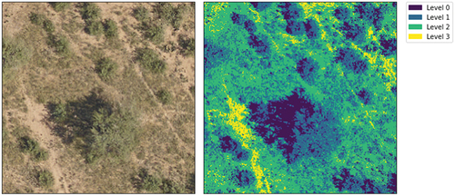
Table A1. Error of omission and commission for the supervised pure pixel classification of the 0.1 camera images that will be used as a reference dataset to evaluate the 1 m classified image (sample size 333).

	Tall woody plants	herbaceous vegetation	Other
Error of commission (%)	15.7	17.1	13.8
Error of omission (%)	7.6	23.7	12.7

Appendix C:

Testing Endmember Extraction Algorithms

Among the most widely used endmember extraction algorithms, the automatic Target Generation Process (ATGP) method can identify endmembers with the least computation time, whereas the N-finder algorithm (N-FINDR) method can extract endmember signatures more accurately but with the highest computation time (Wu and Tsuei 2013). ATGP repeatedly searches for dissimilar signatures and assigns them as new endmembers using a signature similarity metric until it finds signatures for the number of predefined endmembers. N-FINDR uses a maximum noise fraction transformation – i.e. initial endmember signatures are randomly selected and then based on a volume calculation in each pixel the endmembers are replaced based on volume increase as the maximum volume is from the purest pixel than any other combinations of pixels (Wu and Tsuei 2013; Winter 1999). As we have a large volume of data to classify, we needed a method that is fast as well as accurate. Therefore, we tested both the ATGP and N-FINDR methods on a single tile to see which one will be more appropriate to apply over the whole study area. We created fCover maps based on endmember signatures extracted by both methods for the raw tiles and visually inspected the woody plant fractional cover maps. From the visual inspection we found that the map created with the ATGP algorithm has shadow and noise effects whereas the map created with the N-FINDR method does not have this issue. Therefore, we choose the N-FINDR method to extract endmember signatures.

References

- Ahlstrom, A., M. R. Raupach, G. Schurgers, B. Smith, A. Arneth, M. Jung, M. Reichstein, et al. 2015. ”The Dominant Role of Semi-Arid Ecosystems in the Trend and Variability of the Land CO2 Sink.” Science. doi:10.1126/science.aaa1668.
- Alonzo, M., J. P. McFadden, D. J. Nowak, and D. A. Roberts. 2016. “Mapping Urban Forest Structure and Function Using Hyperspectral Imagery and Lidar Data.” Urban Forestry & Urban Greening 17: 135–147. doi:10.1016/j.ufug.2016.04.003.
- Archer, S. R., E. M. Andersen, K. I. Predick, S. Schwinning, R. J. Steidl, and S. R. Woods. 2017. “Woody Plant Encroachment: Causes and Consequences.” Rangeland Systems. doi:10.1007/978-3-319-46709-2_2.
- Asner, G. P. and D. B. Lobell. 2000. “A Biogeophysical Approach for Automated SWIR Unmixing of Soils and Vegetation.” Remote Sensing of Environment 74: 99–112. doi:10.1016/s0034-4257(00)00126-7.
- Asner, G. P. and K. B. Heidebrecht. 2002. “Spectral Unmixing of Vegetation, Soil and Dry Carbon Cover in Arid Regions: Comparing Multispectral and Hyperspectral Observations.” International Journal of Remote Sensing 23: 3939–3958. doi:10.1080/01431160110115960.
- Asner, G. P., D. E. Knapp, T. Kennedy-Bowdoin, M. O. Jones, R. E. Martin, J. Boardman, and R. F. Hughes. 2008. “Invasive Species Detection in Hawaiian Rainforests Using Airborne Imaging Spectroscopy and LiDar.” Remote Sensing of Environment. doi:10.1016/j.rse.2007.11.016.
- Asner, G. P., S. R. Levick, and I. P. J. Smit. 2011. “Remote Sensing of Fractional Cover and Biochemistry in Savannas.” In Ecosystem Function in Savannas: Measurement and Modeling at Landscape to Global Scales, edited by M. J. Hill and N. P. Hanan. Boca Raton, FL: CRC Press. doi:10.1201/b10275.
- Barger, N. N., S. R. Archer, J. L. Campbell, C.-Y. Huang, J. A. Morton, and A. K. Knapp. 2011. “Woody Plant Proliferation in North American Drylands: A Synthesis of Impacts on Ecosystem Carbon Balance.” Journal of Geophysical Research 116. doi:10.1029/2010jg001506.
- Belgiu, M. and L. Drăguţ. 2016. “Random Forest in Remote Sensing: A Review of Applications and Future Directions.” ISPRS Journal of Photogrammetry and Remote Sensing 114: 24–31.
- Belnap, J., B. Weber, and B. Büdel. 2016. “Biological Soil Crusts as an Organizing Principle in Drylands.” Biological Soil Crusts: An Organizing Principle in Drylands. doi:10.1007/978-3-319-30214-0_1.
- Biederman, J. A., R. L. Scott, T. W. Bell, D. R. Bowling, S. Dore, J. Garatuza-Payan, T. E. Kolb, et al. 2017. ”CO Exchange and Evapotranspiration Across Dryland Ecosystems of Southwestern North America.” Global Change Biology 23 (10): 4204–4221.
- Brandt, M., P. Hiernaux, T. Tagesson, A. Verger, K. Rasmussen, A. Aziz Diouf, C. Mbow, E. Mougin, and R. Fensholt. 2016. “Woody Plant Cover Estimation in Drylands from Earth Observation Based Seasonal Metrics.” Remote Sensing of Environment 172: 28–38. doi:10.1016/j.rse.2015.10.036.
- Brandt, M., C. J. Tucker, A. Kariryaa, K. Rasmussen, C. Abel, J. Small, J. Chave, et al. 2020. ”An Unexpectedly Large Count of Trees in the West African Sahara and Sahel.” Nature 587 (7832): 78–82. doi:10.1038/s41586-020-2824-5.
- Clark, M. L., D. A. Roberts, J. J. Ewel, and D. B. Clark. 2011. “Estimation of Tropical Rain Forest Aboveground Biomass with Small-Footprint Lidar and Hyperspectral Sensors.” Remote Sensing of Environment 115: 2931–2942. doi:10.1016/j.rse.2010.08.029.
- Colditz, R. 2015. “An Evaluation of Different Training Sample Allocation Schemes for Discrete and Continuous Land Cover Classification Using Decision Tree-Based Algorithms.” Remote Sensing 7: 9655–9681. doi:10.3390/rs70809655.
- Colgan, M., C. Baldeck, J.-B. Féret, and G. Asner. 2012. “Mapping Savanna Tree Species at Ecosystem Scales Using Support Vector Machine Classification and BRDF Correction on Airborne Hyperspectral and LiDar Data.” Remote Sensing 4: 3462–3480. doi:10.3390/rs4113462.
- Congalton, R. G. and K. Green. 2019. Assessing the Accuracy of Remotely Sensed Data: Principles and Practices. 3rd ed. Boca Raton: CRC Press.
- Dashti, H., N. F. Glenn, S. Ustin, J. J. Mitchell, Y. Qi, N. T. Ilangakoon, A. N. Flores, et al. 2019. “Empirical Methods for Remote Sensing of Nitrogen in Drylands May Lead to Unreliable Interpretation of Ecosystem Function.” IEEE Transactions on Geoscience and Remote Sensing. doi:10.1109/tgrs.2018.2889318.
- Dashti, H., A. Poley, N. F. Glenn, N. Ilangakoon, L. Spaete, D. Roberts, J. Enterkine, A. N. Flores, S. L. Ustin, and J. J. Mitchell. 2019. “Regional Scale Dryland Vegetation Classification with an Integrated Lidar-Hyperspectral Approach.” Remote Sensing. doi:10.3390/rs11182141.
- Dettweiler-Robinson, E., M. Nuanez, and M. E. Litvak. 2018. ”Biocrust Contribution to Ecosystem Carbon Fluxes Varies Along an Elevational Gradient.” Ecosphere 9 (6): e02315. Wiley doi:10.1002/ecs2.2315.
- Devine, A. P., R. A. McDonald, T. Quaife, and I. M. D. Maclean. 2017. “Determinants of Woody Encroachment and Cover in African Savannas.” Oecologia 183 (4): 939–951. doi:10.1007/s00442-017-3807-6.
- Eldridge, D. J., S. Reed, S. K. Travers, M. A. Bowker, F. T. Maestre, J. Ding, C. Havrilla, et al. 2020. ”The Pervasive and Multifaceted Influence of Biocrusts on Water in the World’s Drylands.” Global Change Biology 26 (10): 6003–6014. doi:10.1111/gcb.15232.
- France, G., D. Hooftman, F. van Langevelde, E. Veenendaal, M. W. Steven, and J. Lloyd. 2017. ”MODIS VCF Should Not Be Used to Detect Discontinuities in Tree Cover Due to Binning Bias. A Comment on Hanan Et Al. (2014) and Staver and Hansen (2015).” Global Ecology and Biogeography: A Journal of Macroecology 26 (7): 854–859. Wiley.
- Gallery, W. 2014. NEON Imaging Spectrometer Level 1B Calibrated Radiance. NEON.DOC.001210vA. NEON (National Ecological Observatory Network).
- Gallery, W. 2019. NEON Algorithm Theoretical Basis Document(atbd):Cameramosaic. NEON.DOC.005052vA. NEON (National Ecological Observatory Network).
- Gao, L., Z. Han, D. Hong, B. Zhang, and J. Chanussot. 2022. “CyCu-Net: Cycle-Consistency Unmixing Network by Learning Cascaded Autoencoders.” IEEE Transactions on Geoscience and Remote Sensing. doi:10.1109/tgrs.2021.3064958.
- Gao, L., Z. Wang, L. Zhuang, H. Yu, B. Zhang, and J. Chanussot. 2022. “Using Low-Rank Representation of Abundance Maps and Nonnegative Tensor Factorization for Hyperspectral Nonlinear Unmixing.” IEEE Transactions on Geoscience and Remote Sensing. doi:10.1109/tgrs.2021.3065990.
- Gillan, J. K., G. E. Ponce‐campos, T. L. Swetnam, A. Gorlier, P. Heilman, and M. P. McClaran. 2021. “Innovations to Expand Drone Data Collection and Analysis for Rangeland Monitoring.” Ecosphere 12. doi:10.1002/ecs2.3649.
- Gornish, E. S., H. Ganjurjav, M. Liang, J. L. Simonis, and M. P. McClaran. 2021. ”Identifying Restoration Opportunities Beneath Native Mesquite Canopies.” Restoration Ecology 29: 2. Wiley. doi:10.1111/rec.13334.
- Goulden, T. 2018. L3 Discrete LiDar Processing and QA Informan on for 2018 SRER 2. NEON AOP QA Report. NEON (National Ecological Observatory Network).
- Goulden, T. and Scholl V.2019. NEON Algorithm Theoretical Basis Document (ATBD): Ecosystem Structure. NEON.DOC.002387vA. NEON (National Ecological Observatory Network).
- Han, Z., D. Hong, L. Gao, B. Zhang, and J. Chanussot. 2021. “Deep Half-Siamese Networks for Hyperspectral Unmixing.” IEEE Geoscience and Remote Sensing Letters. doi:10.1109/lgrs.2020.3011941.
- Han, Z., D. Hong, L. Gao, J. Yao, B. Zhang, and J. Chanussot. 2022. “Multimodal Hyperspectral Unmixing: Insights from Attention Networks.” IEEE Transactions on Geoscience and Remote Sensing. doi:10.1109/tgrs.2022.3155794.
- Hansen, M. C., R. S. DeFries, J. R. G. Townshend, M. Carroll, C. Dimiceli, and R. A. Sohlberg. 2003. “Global Percent Tree Cover at a Spatial Resolution of 500 Meters: First Results of the MODIS Vegetation Continuous Fields Algorithm.” Earth Interactions. doi:10.1175/1087-3562(2003)007<0001:gptcaa>2.0.co;2.
- Hartley, A. J., N. MacBean, G. Georgievski, and S. Bontemps. 2017. ”Uncertainty in Plant Functional Type Distributions and Its Impact on Land Surface Models.” Remote Sensing of Environment 203 (December): 71–89. Elsevier. 10.1016/j.rse.2017.07.037.
- Heylen, R., M. Parente, and P. Gader. 2014. “A Review of Nonlinear Hyperspectral Unmixing Methods.” IEEE Journal of Selected Topics in Applied Earth Observations and Remote Sensing. doi:10.1109/jstars.2014.2320576.
- Hill, L. J. R., J.-P. Guerschman, A. S. Marks, and D. J. Barrett. 2013. ”Use of Vegetation Index ‘Fingerprints’ from Hyperion Data to Characterize Vegetation States Within Land Cover/land Use Types in an Australian Tropical Savanna.” IEEE Journal of Selected Topics in Applied Earth Observations and Remote Sensing 6 (2): 309–319. Institute of Electrical and Electronics Engineers (IEEE) doi:10.1109/JSTARS.2012.2222873.
- Hong, D., L. Gao, J. Yao, N. Yokoya, J. Chanussot, U. Heiden, and B. Zhang. 2021. “Endmember-Guided Unmixing Network (EGU-Net): A General Deep Learning Framework for Self-Supervised Hyperspectral Unmixing.” IEEE Transactions on Neural Networks and Learning Systems. doi:10.1109/tnnls.2021.3082289.
- Hong, D., L. Gao, N. Yokoya, J. Yao, J. Chanussot, Q. Du, and B. Zhang. 2021. “More Diverse Means Better: Multimodal Deep Learning Meets Remote-Sensing Imagery Classification.” IEEE Transactions on Geoscience and Remote Sensing. doi:10.1109/tgrs.2020.3016820.
- Huang, C.-Y., S. E. Marsh, M. P. McClaran, and S. R. Archer. 2007. “Postfire Stand Structure in a Semiarid Savanna: Cross-Scale Challenges Estimating Biomass.” Ecological Applications: A Publication of the Ecological Society of America 17 (7): 1899–1910. doi:10.1890/06-1968.1.
- Huang, C.-Y., S. R. Archer, M. P. McClaran, and S. E. Marsh. 2018. “Shrub Encroachment into Grasslands: End of an Era?” PeerJ 6 (September): e5474. doi:10.7717/peerj.5474.
- Jia, K., S. Liang, S. Liu, Y. Li, Z. Xiao, Y. Yao, B. Jiang, et al. 2015. ”Global Land Surface Fractional Vegetation Cover Estimation Using General Regression Neural Networks from MODIS Surface Reflectance.” IEEE Transactions on Geoscience and Remote Sensing: A Publication of the IEEE Geoscience and Remote Sensing Society 539:4787–4796. Institute of Electrical and Electronics Engineers (IEEE). 10.1109/TGRS.2015.2409563
- Jiapaer, G., X. Chen, and A. Bao. 2011. ”A Comparison of Methods for Estimating Fractional Vegetation Cover in Arid Regions.” Agricultural and Forest Meteorology 151 (12): 1698–1710. Elsevier BV.
- Karpowicz, B. and Kampe T. 2015. NEON Imaging Spectrometer Radiance to Reflectance Algorithm Theoretical Basis Document. NEON.DOC.001288vA. NEON (National Ecological Observatory Network).
- Khosravipour, A., A. K. Skidmore, M. Isenburg, T. Wang, and Y. A. Hussin. 2014. “Generating Pit-Free Canopy Height Models from Airborne Lidar.” Photogrammetric Engineering & Remote Sensing 80: 863–872. doi:10.14358/pers.80.9.863.
- Lunt, I. D., L. M. Winsemius, S. P. McDonald, J. W. Morgan, and R. L. Dehaan. 2010. “How Widespread is Woody Plant Encroachment in Temperate Australia? Changes in Woody Vegetation Cover in Lowland Woodland and Coastal Ecosystems in Victoria from 1989 to 2005.” Journal of Biogeography 37: 722–732. doi:10.1111/j.1365-2699.2009.02255.x.
- MacBean, N., R. L. Scott, J. A. Biederman, P. Peylin, T. Kolb, M. E. Litvak, P. Krishnan, et al. 2021. ”Dynamic Global Vegetation Models Underestimate Net CO2 Flux Mean and Inter-Annual Variability in Dryland Ecosystems.” Environmental Research Letters. doi:10.1088/1748-9326/ac1a38.
- Maestre, F. T., C. Escolar, M. Ladrón Guevara, J. L. Quero, R. Lázaro, M. Delgado-Baquerizo, V. Ochoa, M. Berdugo, B. Gozalo, and A. Gallardo. 2014. ”Changes in Biocrust Cover Drive Carbon Cycle Responses to Climate Change in Drylands.” Global Change Biology 20 (8): 2697–2698. Wiley doi:10.1111/gcb.12659.
- Maggiori, E., A. Plaza, and Y. Tarabalka. 2018. “Models for Hyperspectral Image Analysis: From Unmixing to Object-Based Classification.” Mathematical Models for Remote Sensing Image Processing. doi:10.1007/978-3-319-66330-2_2.
- Marconi, S., S. J. Graves, B. G. Weinstein, S. Bohlman, and E. P. White. 2021. “Estimating Individual-Level Plant Traits at Scale.” Ecological Applications: A Publication of the Ecological Society of America 31 (4): e02300. doi:10.1002/eap.2300.
- McClaran, M. P. 2003. “A Century of Vegetation Change on the Santa Rita Experimental Range.” In Santa Rita Experimental Range: 100 Years (1903 to 2003) of Accomplishments and Contributions. Proceedings RMRS-P-30. Ogden, UT: US Department of Agriculture Forest Service.
- Millard, K. and M. Richardson. 2015. “On the Importance of Training Data Sample Selection in Random Forest Image Classification: A Case Study in Peatland Ecosystem Mapping.” Remote Sensing 7 (7): 8489–8515.
- Mishra, N. B. and K. A. Crews. 2014. ”Estimating Fractional Land Cover in Semi-Arid Central Kalahari: The Impact of Mapping Method (Spectral Unmixing Vs. Object-Based Image Analysis) and Vegetation Morphology.” Geocarto International 29 (8): 860–877. Informa UK Limited.
- Myers-Smith, I. H., B. C. Forbes, M. Wilmking, M. Hallinger, T. Lantz, D. Blok, K. D. Tape, et al. 2011. ”Shrub Expansion in Tundra Ecosystems: Dynamics, Impacts and Research Priorities”. Environmental Research Letters 6: 045509. doi:10.1088/1748-9326/6/4/045509.
- Naidoo, L., M. A. Cho, R. Mathieu, and G. Asner. 2012. ”Classification of Savanna Tree Species, in the Greater Kruger National Park Region, by Integrating Hyperspectral and LiDar Data in a Random Forest Data Mining Environment.” ISPRS Journal of Photogrammetry and Remote Sensing: Official Publication of the International Society for Photogrammetry and Remote Sensing 69 April, Elsevier BV: 167–179. 10.1016/j.isprsjprs.2012.03.005.
- National Land Cover Database (NLCD). 2020. 2016 Shrubland Fractional Components for the Western U.S. (Ver. 3.0, July 2020). 10.5066/P9MJVQSQ.
- Scott, R. L., J. A. Biederman, E. P. Hamerlynck, and G. A. Barron-Gafford. 2015. ”The Carbon Balance Pivot Point of Southwestern U.S. Semiarid Ecosystems: Insights from the 21st Century Drought.” Journal of Geophysical Research: Biogeosciences 120 (12): 2612–2624. American Geophysical Union (AGU).
- Smith, W. K., M. P. Dannenberg, D. Yan, S. Herrmann, M. L. Barnes, G. A. Barron-Gafford, J. A. Biederman, et al. 2019. ”Remote Sensing of Dryland Ecosystem Structure and Function: Progress, Challenges, and Opportunities”. Remote Sensing of Environment 233: 111401. doi:10.1016/j.rse.2019.111401.
- Staver, A. C. and C. H. Matthew. 2015. ”Analysis of Stable States in Global Savannas: Is the CART Pulling the Horse? - a Comment.” Global Ecology and Biogeography: A Journal of Macroecology 24 (8): 985–987. Wiley doi:10.1111/geb.12285.
- Staver, A., A. Carla, C. Staver, J. Botha, and L. Hedin. 2017. “Soils and Fire Jointly Determine Vegetation Structure in an African Savanna.” The New Phytologist 216: 1151–1160. doi:10.1111/nph.14738.
- Swatantran, A., R. Dubayah, D. Roberts, M. Hofton, and J. Bryan Blair. 2011. “Mapping Biomass and Stress in the Sierra Nevada Using Lidar and Hyperspectral Data Fusion.” Remote Sensing of Environment 115: 2917–2930. doi:10.1016/j.rse.2010.08.027.
- Tiribelli, F., T. Kitzberger, and J. Manuel Morales. 2018. ”Changes in Vegetation Structure and Fuel Characteristics Along Post-Fire Succession Promote Alternative Stable States and Positive Fire-Vegetation Feedbacks.” Journal of Vegetation Science: Official Organ of the International Association for Vegetation Science 29 (2): 147–156. Wiley.
- Ustin, S. L., D. A. Roberts, J. A. Gamon, G. P. Asner, and R. O. Green. 2004. ”Using Imaging Spectroscopy to Study Ecosystem Processes and Properties.” Bioscience 54: 6–523. Oxford University Press (OUP). doi:10.1641/0006-3568(2004)054[0523:UISTSE]2.0.CO;2.
- Varga, T. A. and G. P. Asner. 2008. “Hyperspectral and LiDar Remote Sensing of Fire Fuels in Hawaii Volcanoes National Park.” Ecological Applications: A Publication of the Ecological Society of America 18 (3): 613–623. doi:10.1890/07-1280.1.
- Venter, Z. S., M. D. Cramer, and H.-J. Hawkins. 2018. “Drivers of Woody Plant Encroachment Over Africa.” Nature Communications 9 (1): 2272. doi:10.1038/s41467-018-04616-8.
- Wanner, W., X. Li, and A. H. Strahler. 1995. “On the Derivation of Kernels for Kernel-Driven Models of Bidirectional Reflectance.” Journal of Geophysical Research. doi:10.1029/95jd02371.
- Winter, M. E. 1999. “N-FINDR: An Algorithm for Fast Autonomous Spectral End-Member Determination in Hyperspectral Data.” Imaging Spectrometry V. doi:10.1117/12.366289.
- Wu, J.-C. and G.-C. Tsuei. 2013. “Comparison of Hyperspectral Endmember Extraction Algorithms.” Journal of Applied Remote Sensing 7: 073525. doi:10.1117/1.jrs.7.073525.
- Xiao, J. and A. Moody. 2005. ”A Comparison of Methods for Estimating Fractional Green Vegetation Cover Within a Desert-To-Upland Transition Zone in Central New Mexico, USA.” Remote Sensing of the Environment 98: 2–3–250237–250. Elsevier BV.
- Yang, L., S. Jin, P. Danielson, C. Homer, L. Gass, S. M. Bender, A. Case, et al. 2018. ”A New Generation of the United States National Land Cover Database: Requirements, Research Priorities, Design, and Implementation Strategies”. ISPRS Journal of Photogrammetry and Remote Sensing 146: 108–123. doi:10.1016/j.isprsjprs.2018.09.006.
- Yang, X. and K. A. Crews. 2019. ”Fractional Woody Cover Mapping of Texas Savanna at Landsat Scale.” Land 8: 1–9. Multidisciplinary Digital Publishing Institute. doi:10.3390/land8010009.
- Zhang, W., M. Brandt, Q. Wang, A. V. Prishchepov, C. J. Tucker, Y. Li, H. Lyu, and R. Fensholt. 2019. “From Woody Cover to Woody Canopies: How Sentinel-1 and Sentinel-2 Data Advance the Mapping of Woody Plants in Savannas.” Remote Sensing of Environment. doi:10.1016/j.rse.2019.111465.