LWIR hyperspectral image classification based on a temperature-emissivity residual network and conditional random field model

ABSTRACT

Long-wave infrared (LWIR) hyperspectral images can provide temperature and emissivity information, and have unique advantages in classification tasks, especially in the fields of minerals, vegetation, and man-made materials. However, LWIR image acquisition is greatly affected by the atmosphere, which results in obvious spectral noise. Meanwhile, field-based and aerial thermal infrared hyperspectral images are faced with problems such as spatial heterogeneity and salt-and-pepper noise, which results in the traditional spectral-based and object-oriented classification methods performing poorly in the classification task. In this paper, using the emissivity spectra and land surface temperature inversed from LWIR hyperspectral images, a classification framework based on a temperature-emissivity residual network and conditional random field model (TERN-CRF) is proposed. In this method, the residual network is designed to extract and fuse in-depth spectral and local spatial features, and the conditional random field (CRF) model incorporates the spatial-contextual information by the use of the temperature information, to improve the problem of voids and isolated regions in the classification map. To validate the performance of the proposed method, three LWIR datasets acquired by the Hyper-Cam sensor were used in the experiments: an aerial dataset and two field-based datasets of minerals and leaves. The experimental classification results obtained using the LWIR datasets confirm the performance of the proposed TERN-CRF classification method, which is shown to be superior to the traditional hyperspectral image classification methods and a CNN-based method. Furthermore, the CRF post-processing part can effectively alleviate the isolated regions in the classification map.

KEYWORDS:

• Fourier-transformed long-wave infrared hyperspectral imagery
• spectral emissivity
• conditional random field model
• deep learning
• classification

1. Introduction

Long-wave infrared (LWIR) hyperspectral sensors acquire the energy radiated across the range of the 8–14 μm spectrum (Adler-Golden et al. 2014). In contrast to visible imagery, LWIR imagery can be imaged day and night, with no observation time constraints, and LWIR hyperspectral images contain fine emissivity and temperature information. Temperature is the manifestation of thermal energy, where the higher the temperature, the higher the corresponding energy emitted. The spatial distribution of temperature also correlates with the type of ground cover. Emissivity reflects the ability of objects to emit thermal radiation at various wavelengths, and is directly related to the composition and physical properties of the objects (Zhu et al. 2021). Minerals and vegetation are two typical materials whose emissivity has unique spectral characteristics in the LWIR band (Manolakis et al. 2019). To be specific, the vibrations of the silica-valent electrons in silicate minerals show distinctive spectral features in the LWIR band, whereas these minerals do not have obvious spectral features in the visible and near-infrared (NIR) band (Hunt 2012). LWIR-based studies of trees and their leaves have shown that the spectra of leaves are mainly controlled by the structural compounds in the leaf surface (Luz and Crowley 2007). These compounds include cellulose, hemicellulose, cuticle, silica, and terpenes, which have emissivity characteristics that enhance species separability. Since LWIR imagery has unique advantages in the classification of ground objects, especially minerals and vegetation, and silicate minerals and vegetation are the main components of the land surface, this gives LWIR hyperspectral remote sensing imagery high potential value for land-surface classification tasks. Therefore, it is of great significance to extract the emissivity and temperature information from LWIR hyperspectral imagery, and to classify ground objects based on the temperature and emissivity information.

With the development of LWIR hyperspectral instruments, research into classification based on different sensors and data has been undertaken. A spatially enhanced broadband array spectrograph system (SEBASS) was the first LWIR hyperspectral instrument to be used for mineral mapping (Kirkland et al. 2002). SEBASS-based mineral mapping has demonstrated the effectiveness of LWIR hyperspectral imagery in the field of minerals, to better distinguish the subclasses of minerals with subtle spectral differences (Kirkland et al. 2002; Vaughan, Calvin and Taranik 2003; Vaughan et al. 2005; Aslett, Taranik and Riley 2017). With the introduction of commercial LWIR hyperspectral instruments, LWIR hyperspectral data are becoming more widely used. The Specim AisaOWL LWIR hyperspectral sensor was applied to map surface quartz content by acquiring day and night airborne images of the observation area from an aerial platform, and a decision tree was then used to produce a quartz content map (Weksler, Rozenstein and Ben-Dor 2018). The Bruker VERTEX 70 Fourier transform infrared (FTIR) spectrometer, which is a fully digital infrared spectrometer, has been used in several studies for vegetation subclass classification (Ullah et al. 2012; Harrison, Rivard and Sánchez-Azofeifa 2018; Rivard and Sánchez-Azofeifa 2018). The use of the FTIR spectrometer to measure the emissivity spectra of the leaves of trees shows that LWIR hyperspectral data have great potential for accurate vegetation classification. The Fourier transform based LWIR hyperspectral imager developed by Telops – the Hyper-Cam – was first used for vegetation species identification, and the overall accuracy of the LWIR classification was found to be better than that of visible imagery classification (Rock et al. 2016). A dataset of LWIR hyperspectral data captured by the Hyper-Cam device was made public in the 2014 IEEE Data Fusion Contest. The traditional classification methods based on the existing visible NIR hyperspectral images were used for the LWIR hyperspectral data, and the usability of these methods was experimentally demonstrated. However, these traditional methods use only raw radiance images that include atmospheric and environmental radiometric interference, limiting the accuracy of the classification (Barisione et al. 2016; Marwaha, Kumar and Kumar 2015; Pan, Shi and Xu 2017). The HyTES spectrometer represents the highest level of development for LWIR hyperspectral imagers, and has been used by the National Aeronautics and Space Administration (NASA) to determine the optimal infrared (IR) band position for mapping the Earth’s composition (Iqbal et al. 2018).

For the application of LWIR hyperspectral images in classification tasks, ideal classification results cannot be achieved without accurate temperature and emissivity extraction, spectral feature extraction, and the selection of a suitable classifier. Due to the relatively high noise level of LWIR hyperspectral imagery, the extensive classification work started with the use of minimum noise fraction (MNF) transformation (Vaughan, Calvin and Taranik 2003; Vaughan et al. 2005; Aslett, Taranik and Riley 2017; Marwaha, Kumar and Kumar 2015) and principal component analysis (PCA) (Rivard and Sánchez-Azofeifa 2018), to enhance the spectral features and reduce the data dimensionality. Spectral matching techniques have also been widely used for LWIR hyperspectral classification, for which the aim is to test the spectral characteristics by expressing the similarity of the reference spectra. The two most widely used techniques are the spectral angle mapper (SAM) (Vaughan, Calvin and Taranik 2003; Rivard and Sánchez-Azofeifa 2018; Marwaha, Kumar and Kumar 2015; Iqbal et al. 2018) and matched filtering (MF) (Vaughan, Calvin and Taranik 2003; Vaughan et al. 2005; Aslett, Taranik and Riley 2017; Ullah et al. 2012; Rivard and Sánchez-Azofeifa 2018; Marwaha, Kumar and Kumar 2015). Other popular image classification approaches, such as the decision tree (Weksler, Rozenstein and Ben-Dor 2018; Rivard and Sánchez-Azofeifa 2018), support vector machine (Rivard and Sánchez-Azofeifa 2018; Marwaha, Kumar and Kumar 2015) and random forest (RF) (Harrison, Rivard and Sánchez-Azofeifa 2018; Rivard and Sánchez-Azofeifa 2018; Rock et al. 2016) methods, have also been applied to LWIR hyperspectral classification.

Although the traditional methods of spectral matching and machine learning have achieved good classification results for LWIR hyperspectral classification (Yang et al. 2018), most of the methods rely on the modelling of the spectral features, and only extract shallow spectral and spatial features. For the Fourier-transformed LWIR hyperspectral images obtained by the Hyper-Cam imager, although their signal-to-noise ratio and spectral-spatial resolution are higher than those of the other LWIR imagers, the images still have high spectral similarity and spatial heterogeneity, which bring difficulties to the classification task. In recent years, deep learning has been widely used in the field of hyperspectral image classification, due to its powerful computational ability in feature learning, but, limited by the small amount of publicly available datasets, few scholars have applied deep learning to LWIR hyperspectral classification. Convolutional neural networks (CNNs) and their extensions are currently the most commonly used network architectures based on deep learning (Chen et al. 2016; He et al. 2016; Reynolds and Murphy 2007; Zhong et al. 2018). However, although CNNs have been shown to be able to provide optimal inputs for hyperspectral classification, the results of CNNs can lead to isolated regions in the final classification map.

In this study, to make full use of the temperature and emissivity information in Fourier-transformed LWIR hyperspectral imagery for accurate object classification, three standard LWIR hyperspectral classification datasets were built using the Hyper-Cam sensor. A framework based on a temperature-emissivity residual network and CRF model is proposed to overcome the problem of the spectral similarity and spatial heterogeneity in LWIR hyperspectral emissivity images, to obtain more accurate classification results.

The main contributions of this work are as follows.

1. The proposed temperature-emissivity residual network and conditional random field model (TERN-CRF) framework for LWIR hyperspectral classification. For the temperature and emissivity information extracted from the original images, the residual network continuously extracts the spectral and spatial information from the emissivity images, and the spatial-contextual information in the LWIR images is considered based on the temperature map. This framework can not only extract the deep spatial and spectral features in the emissivity images to overcome the difficulties of the spectral similarity and spatial heterogeneity in LWIR emissivity hyperspectral images, but it also uses the temperature map to resolve the isolated misclassified regions in the images, to obtain more accurate classification results.

2. The designed temperature-emissivity residual network framework. The residual linkage in the network alleviates the problem of accuracy degradation with increasing iterations, and this residual linkage is applied to the spectral and spatial feature extraction, which can extract more discriminative features. Batch normalization (BN) is also used to improve the classification results for unbalanced training samples.

3. The construction of three Fourier-transformed LWIR hyperspectral datasets. In order to make full use of the advantages of LWIR hyperspectral data for the classification of minerals and vegetation, three standard datasets were built in this study: a mineral subclass dataset and a tree leaves subclass dataset collected on the ground, and a set of aerial LWIR hyperspectral data for large-scene classification work.

The rest of this paper is composed of five sections. In Section II, the datasets and preprocessing are introduced. Section III provides the details of the proposed TERN-CRF classification framework. The experimental results and analysis are presented in Section IV. Section V is the discussion section. Our conclusions and future work are then summarized in Section VI.

2. Materials

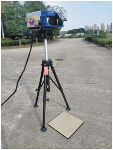
In this section, we describe how the three LWIR datasets (two field-based datasets and one aerial dataset) used in the experiments were built. We also explain how the emissivity and land surface temperature information of the LWIR hyperspectral images was obtained. All these datasets were acquired by the Telops Hyper-Cam sensor, which is shown in Figure 1. The Hyper-Cam is an advanced passive LWIR hyperspectral imaging system based on Fourier transform technology, with not only a high spatial resolution to provide abundant two-dimensional spatial information, but also a high spectral resolution to provide fine three-dimensional spectral data. The spectral range of the Hyper-Cam sensor is 7.7–11.8 μm, the field of view is 6.4° × 5.1°, and the spectral resolution reaches 0.25 cm⁻¹.

Figure 1. The Fourier transform based LWIR hyperspectral imaging system: the Telops Hyper-Cam.

2.1. The Fourier-transformed thermal infrared hyperspectral datasets

(i) Mineral dataset

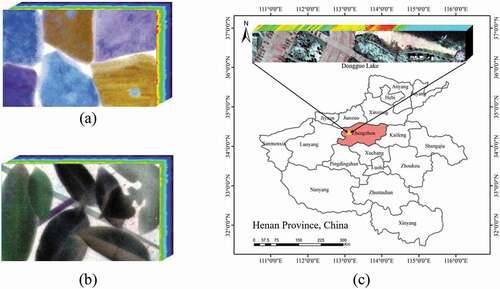
Minerals have unique spectral characteristics in the LWIR band, so that LWIR imagery is widely used for surface mineral mapping. We constructed a benchmark mineral classification dataset. The dataset contains six mineral types: calcite, fibrous gypsum, hard gypsum, dolomite, talc, and diopside. The background concrete floor is also set as a category. At the time of imaging, the Hyper-Cam system was at a height of 1.6 m, with a spectral range of 7.8–11.5 μm, a total of 85 bands, a spectral resolution of 6 cm-1, and a field of view size of 15 cm × 7 cm. Figure 2(a) provides an overview of this dataset.

Figure 2. The three datasets (a) Mineral dataset. (b) Tree leaves dataset. (c) Dongguo Lake dataset.

(ii) Tree leaves dataset

Different trees have different spectral shapes for the different structural compounds on the leaf surface in the LWIR band, which is due to the leaves having different structural compound contents, such as cellulose, hemicellulose, cuticle, silica, and terpenes. This characteristic is advantageous in tree leaves subclass mapping. In this study, a tree leaves dataset was built, as shown in Figure 2(b). This dataset contains seven types of leaves: photinia leaves, evergreen magnolia leaves, grass leaves, camphor leaves, osmanthus leaves, paper mulberry leaves, and glossy privet leaves. Concrete floor is again the background class. The tree leaves dataset is consistent with the shooting parameters of the mineral dataset.

(iii) Dongguo Lake dataset

The Dongguo Lake dataset, as shown in Figure 2(c), is an aerial Fourier-transformed LWIR hyperspectral dataset, which was captured on 30 March 2019, from 10:30–10:48 a.m., at Dongguo Lake, Shangjie District, Zhengzhou, Henan province, China (113°16‘43 “E, 34°49’33 “N). The flight altitude was 2500 m, corresponding to a spatial resolution of 0.9 m. The spectral range was 8–11.5 µm, with 78 bands. During the data acquisition period, the imaging size was 320 × 256 pixels, the weather was clear and cloudless, the temperature was 16°C, and the humidity level was 13%. The study area included houses, roads, sandy areas, water, vegetation, and bare soil.

2.2. Preprocessing

The Hyper-Cam sensor obtains the radiance image directly, but the raw radiance image contains the interference of environmental radiation, and thus cannot reflect the spectral differences between different categories. Different objects have unique emissivity spectra, but different classes also have different heat-absorbing and heat-emitting capabilities. Therefore, it is more effective to use the emissivity and temperature information of LWIR hyperspectral images for classification. The temperature and emissivity information was extracted from the raw radiance images by atmospheric compensation and temperature-emissivity separation, where the atmospheric compensation removes the energy emitted by particles in the atmosphere, and the temperature-emissivity separation solves both the temperature and emissivity parameters by adding constraints.

For the Fourier-transformed LWIR hyperspectral images taken by the Hyper-Cam system, we used the Fast Line-of-sight Atmospheric Analysis of Spectral Hypercubes-Infrared (FLAASH-IR) algorithm, which is an automatic atmospheric compensation and temperature and emissivity separation method, to extract the temperature and emissivity information from the images acquired by the Hyper-Cam system (Adler-Golden et al. 2014). When compared with those methods that rely on accurate atmospheric parameters to obtain precise emissivity and temperature information, FLAASH-IR can automatically compensate the atmospheric information from the original radiance imagery for emissivity and temperature retrieval. In the three Fourier-transformed LWIR hyperspectral datasets built in this study, both the atmospheric compensation of the LWIR hyperspectral imagery and the preprocessing of the temperature and emissivity inversion were completed using FLAASH-IR (Adler-Golden et al. 2014; Liu et al. 2020). The temperature and emissivity images and the average emissivity curves of the features after the application of FLAASH-IR for these three datasets are shown in Figure 3.

Figure 3. Spectra and temperature of the three datasets. (a) Radiance spectra of the mineral dataset classes. (b) Radiance spectra of the tree leaves dataset classes. (c) Radiance spectra of the Dongguo Lake dataset classes. (d) Emissivity spectra of the mineral dataset classes. (e) Emissivity spectra of the tree leaves dataset classes. (f) Emissivity spectra of the Dongguo Lake dataset classes. (g) Temperature of the mineral dataset. (h) Temperature of the tree leaves dataset. (i) Temperature of the Dongguo Lake dataset.

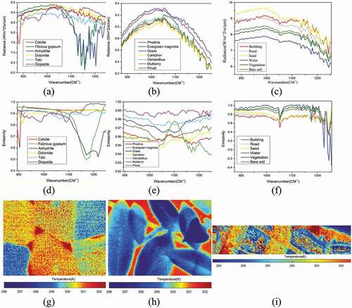
From the emissivity and temperature retrieval results for the mineral dataset, it can be seen that the homogeneity of the mineral temperatures is good in the temperature map, but some temperature inconsistencies do exist in the minerals, due to the unevenness of their surface structures. From the emissivity spectra, it can be seen that the emissivity spectra of the various minerals have different characteristics, especially calcite, talc and hard gypsum, which have distinct spectral absorption bands. Although fibrous gypsum, dolomite, and diopside do not have obvious spectral absorption features, they do have obvious differences in their spectral curves.

From the emissivity and temperature retrieval results for the tree leaves dataset, it can be seen that the temperature of the leaves is much lower than that of the background concrete ground in the temperature map. From the emissivity spectra, it can be seen that the ranges of the values for the different vegetation types are quite different. This indicates that the emissivity can better characterize the attributes of the leaves than the original radiance spectra.

For the Dongguo Lake dataset, the temperature of the buildings, roads, sand, and bare soil is higher, while the temperature of vegetation and water is lower. The temperature distributions of the different features are also very different, with obvious temperature boundaries, but the distribution of the temperature is inhomogeneous. The contrast of the different features is lower in the emissivity images than in the original radiance images from the same band, and it is difficult to distinguish the feature boundaries and feature types visually. Although the results of the temperature and emissivity extraction based on FLAASH-IR for the thermal infrared hyperspectral images of this aerial dataset are not ideal, the emissivity spectra of the different features are distinguishable, to some extent.

Based on the above temperature-emissivity retrieval results, it can be seen that the emissivity spectra can better characterize the essential attributes of materials, and are more distinguishable than the original radiance spectra. Moreover, the temperatures of different types of land surfaces are quite different, and it is an effective way to distinguish different types of land surfaces. In our work, both the temperature and emissivity features were utilized in the classification.

3. The TERN-CRF framework for LWIR hyperspectral image classification

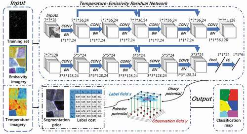
In this section, the temperature-emissivity residual network and CRF model proposed for Fourier-transformed LWIR hyperspectral images are described. Figure 4 shows the overall flowchart of the TERN-CRF framework. TERN-CRF consists of two main steps: i) construction of the temperature-emissivity residual network model; and ii) post-processing based on the CRF model. Firstly, the TERN model is proposed to extract the deep spectral and spatial features from the emissivity images, and then the output probability images are used as the input of the unary potential term of the CRF model.

Figure 4. Flowchart of the proposed TERN-CRF method. The model includes two steps: the temperature-emissivity residual network and post-processing based on the CRF model. The network includes two spectral and two spatial residual blocks, an average pooling layer, and a fully connected layer. The CRF model includes a segmentation prior and inference of CRF.

3.1. The TERN model for LWIR hyperspectral image classification

The TERN model uses batch-normalized three-dimensional (3-D) convolutional layers, residual blocks, average pooling layers, and fully connected (FC) layers to extract fused deep spectral features and local spatial features. All the labelled samples are divided into three groups: a training group, a validation group, and a test group. In order to better utilize the spectral and spatial features of LWIR hyperspectral images, the network uses data cubes of size $w\times w\times b$ in the emissivity images as the input terms, and the label vectors corresponding to the training group $Z^1$, the validation group $Z^2$, and the test group$Z^3$ are $Y^1$, $Y^2$, and $Y^3$, respectively. In this way, the training process updates the parameters of the TERN model until the model is able to obtain higher-accuracy predictions ${\hat{Y}}^3$for the ground-truth labels $Y^3$ of the surface of a given neighbouring cube $Z^3$.

After the architecture of the deep learning model is built and the hyperparameters for the training are configured, the model is trained for hundreds of epochs using the training group $Z^1$ and their ground-truth label vector set$\hspace{0.17em}{Y}^1$. In this process, the parameters in the TERN model are updated by inverting the gradient of the cross-entropy objective function in (1), which represents the difference between the predicted label vector $\hat{y}=\left[{\hat{y}}_1,{\hat{y}}_2,\dots ,{\hat{y}}_L\right]$and the ground-truth label vector $y_l=\left[y_1,y_2,\dots ,y_L\right]$.

(1) $C\left(\hat{y},y_l\right)=\sum _{i=1}^L{y}_i\left(log\sum _{j=1}^L{e}^{{\hat{y}}_j}-{\hat{y}}_i\right)$(1)

The validation group $Z^2$ is used to monitor the training process and select the network with the highest classification accuracy by measuring the classification performance of the interim model, which is the intermediate network generated during the training phase. Finally, the test group $Z^3$ is used to evaluate the generality of the trained TERN model by computing the classification metrics and visualizing the topic maps.

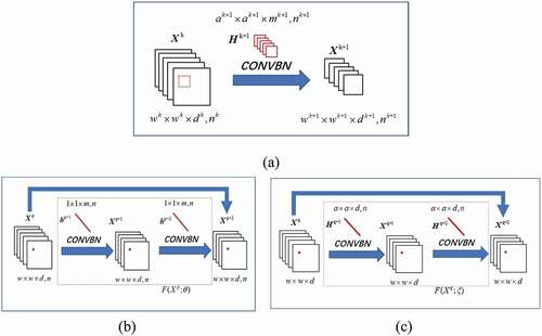
(i) Three-dimensional convolutional layers with batch normalization

3-D convolutional layers are used as the basic elements of the TERN model. BN is also performed in each convolutional layer (CONVBN) of the TERN model. This strategy makes the training process of the deep learning model more efficient. As shown in Figure 5, if the $\left(k+1\right)\mathrm{t}\mathrm{h}$ 3-D convolutional layer has $n^k$ input feature cubes of size $w^k\times w^k\times d^k$, and the convolutional filter bank contains $n^{k+1}$ convolutional filters of size$a^{k+1}\times a^{k+1}\times m^{k+1}$ with subsampling steps $\left(s_1,s_1,s_2\right)$ for convolution operations, the layer produces $n^{k+1}$ output feature cubes of size $w^{k+1}\times w^{k+1}\times d^{k+1}$, where the spatial width $w^{k+1}=\left[1+\left(w^k-a^{k+1}\right)/s_1\right]$ and the spectral depth $d^{k+1}=\left[1+\left(d^k-m^{k+1}\right)/s_2\right]$. The $i\mathrm{t}\mathrm{h}$output of the CONVBN of the $\left(k+1\right)\mathrm{t}\mathrm{h}$ 3-D convolutional layer can be formulated as:

(2) $X_i^{k+1}=R\left(\sum _{j=1}^{n^k}{\hat{X}}_j^k\ast H_i^{k+1}+b_i^{k+1}\right)$(2)

(3) ${\hat{X}}^k=\frac{X^k-E\left(X^k\right)}{Var\left(X^k\right)}$(3)

Figure 5. (a), (b) and (c) respectively represent three-dimensional CONVBN, spectral residual blocks and spatial residual blocks.

where $X_j^k\in {\mathbb{R}}^{w\times w\times d}$ is the $j\mathrm{t}\mathrm{h}$ input feature tensor of the $\left(k+1\right)\mathrm{t}\mathrm{h}$ layer; ${\hat{X}}^k$ is the normalization result of the batch feature cubes $X^k$in the kth layer; and $E\left(\cdot \right)$ and $Var\left(\cdot \right)$represent the expectation and variance function of the input feature tensor, respectively. $H_i^{k+1}$ and $b_i^{k+1}$ denote the parameters and bias of the $i\mathrm{t}\mathrm{h}$ convolutional filter bank in the $\left(k+1\right)\mathrm{t}\mathrm{h}$ layer, $\ast$ represents the 3-D convolution operation, and $R\left(\cdot \right)$ is the rectified linear unit activation function that sets elements with negative numbers to zero.

(ii) Spectral and spatial residual blocks

Although CNN models have been widely used for the classification of hyperspectral images, obtaining great results, the classification accuracy decreases with the increasing number of convolutional layers after convolving several layers (Sminchisescu, Kanaujia and Metaxas 2006). This phenomenon stems from the fact that the representation capability of CNNs is too high compared to the relatively small number of training samples with the same regularization settings. This problem of decreasing accuracy can be mitigated by adding shortcut connections between each layer, to create residual blocks (Cao, Zhou and Li 2016). Due to the high spectral and spatial resolution of LWIR hyperspectral data, two residual blocks are used in the general architecture to continuously extract spectral and spatial features from the original 3-D LWIR hyperspectral cube. This architecture allows the gradients from the higher levels to propagate rapidly back to the lower levels, thus facilitating and normalizing the model training process.

In the spectral residual blocks, convolution kernels of size $1\times 1$ are used for the $p\mathrm{t}\mathrm{h}$ layer and $\left(p+1\right)\mathrm{t}\mathrm{h}$ layer respectively, in the consecutive filter banks $h^{p+1}$and $h^{p+2}$, as shown in Figure 5. At the same time, the spatial size of the 3-D feature cubes $X^{p+1}$ and $X^{p+2}$ is kept constant at $w\times w$ by the padding strategy, which means that the output feature cubes are copied to the padded region with the values in the boundary region after the convolution operation in the spectral dimension. These two convolutional layers then build a residual function $F\left(X^P;\theta \right)$, instead of directly mapping $X^p$ with skip connections. The spectral residual architecture is expressed by (4)–(6):

(4) $X^{P+2}=X^P+F\left(X^P;\theta \right)$(4)

(5) $F\left(X^P;\theta \right)=R\left({\hat{X}}^{P+1}\right)\ast h^{p+2}+b^{p+2}$(5)

(6) $X=R\left({\hat{X}}^{P+1}\right)\ast h^{p+1}+b^{p+1}$(6)

where$\theta =\left\{h^{p+1},h^{p+2},b^{p+1},b^{p+2}\right\}$; $X^{p+1}$ represents the n input 3-D feature cubes of the $\left(p+1\right)\mathrm{t}\mathrm{h}$ layer; and $h^{p+1}$and $b^{p+1}$ denote the spectral convolution kernels and bias in the $\left(p+1\right)\mathrm{t}\mathrm{h}$ layer, respectively. In fact, the convolution kernels $h^{p+1}$and $b^{p+1}$ are composed of one-dimensional (1-D) vectors, which can be regarded as a special case of 3-D convolution kernels. The output tensor of the spectral residual blocks also includes undefined-D feature cubes.

In the spatial residual blocks, as shown in Figure 5, the spatial feature extraction is mainly performed using $n$ 3-D convolution kernels of size $a\times a\times d$ in the consecutive two-layer filter banks $H^{q+1}$ and $H^{q+2}$. The spectral depth $d$ of these kernels is equal to the spectral depth of the input 3-D feature cube $X^q$. The spatial sizes of feature cubes $X^{q+1}$ and $X^{q+2}$ are kept constant at $w\times w$. Thus, the spatial residual architecture is expressed as shown in the following equations:

(7) $X^{q+2}=X^q+F\left(X^q;\xi \right)$(7)

(8) $F\left(X^q;\xi \right)=R\left({\hat{X}}^{q+1}\right)\ast H^{q+2}+b^{q+2}$(8)

(9) $X=R\left({\hat{X}}^{q+1}\right)\ast H^{q+1}+b^{q+1}$(9)

where $\theta =\left\{H^{q+1},H^{q+2},b^{q+1},b^{q+2}\right\}$; $X^{q+1}$ represents the 3-D input feature volume in the $\left(q+1\right)\mathrm{t}\mathrm{h}$ layer; and $H^{q+1}$ and $b^{q+1}$ denote the $n$ spatial convolution kernels in the $\left(q+1\right)\mathrm{t}\mathrm{h}$ layer, respectively. Compared with their spectral counterparts, the convolutional filter banks in the spatial residual blocks are made up of 3-D tensors. The output of this block is a 3-D feature volume.

(iii) The temperature-emissivity residual network

As LWIR hyperspectral images contain one spectral dimension and two spatial dimensions, we propose a framework for successive extraction of the spectral and spatial features for pixel-wise classification of LWIR hyperspectral images. As shown in Figure 4, the TERN model includes a spectral feature learning part, a spatial feature learning part, a mean pooling layer, and an FC layer. Compared with a CNN, the TERN model mitigates the accuracy degradation by formulating the hierarchical feature representation layers as continuous residual blocks by adding skip connections between every other layer.

Taking the LWIR hyperspectral image of Dongguo Lake as an example, the 3-D sample size is 7 × 7 × 78. The spectral feature learning part includes two convolutional layers and two spectral residual blocks. In the first convolutional layer, 24 1 × 1 × 7 spectral kernels are convolved in the input volume to generate 24 7 × 7 × 36 feature cubes. The 1 × 1 × 7 vector kernels are used in these blocks to reduce the high dimensionality of the input cubes and to extract the low-level spectral features of the LWIR hyperspectral imagery. Next, two consecutive spectral residual blocks use 24 1 × 1 × 7 vector kernels to learn the deep spectral representation. The final convolutional layer of this learning section, which includes 128 1 × 1 × 36 spectral kernels for retaining discriminative spectral features, convolves the 24 7 × 7 features in time sequence to produce a 7 × 7 feature volume as input to the spatial feature learning part.

The spatial feature learning part extracts discriminative spatial features using a 3-D convolutional layer and two spatial residual blocks. The first convolutional layer of this part reduces the spatial size of the input feature cube and extracts low-level spatial features using 24 3 × 3 × 128 spatial kernels, resulting in a 5 × 5 × 24 feature tensor output. Then, similar to the spectral part, the two spatial residual blocks learn the deep spatial representation with four convolutional layers, with both blocks using 24 3 × 3 × 24 spatial kernels, and keep the size of the feature cube constant.

After the above two feature learning parts, an average pooling layer (POOL) transforms the extracted 5 × 5 × 24 spectral-spatial feature volume to a 1 × 1 × 24 feature vector. Next, an FC layer adapts the results to the LWIR hyperspectral image dataset according to the number of land-cover categories and generates an output vector $\hat{y}=\left[{\hat{y}}_1,{\hat{y}}_2,\dots ,{\hat{y}}_L\right]$.

3.2. The CRF model for LWIR hyperspectral imagery

The traditional pairwise CRF model (Zhao, Zhong and Zhang 2015) does not consider the distribution characteristics of the image features, resulting in over-smooth classification results. Although the object-oriented segmentation method relies on the choice of scale, it can consider the spatial-contextual information between each object by segmenting the image into multiple object units. However, the TERN model can only utilize local spatial information, which leads to holes or isolated regions in the classification map. The advantages of the object-oriented approach are incorporated into the CRF model to achieve classification mapping of LWIR hyperspectral images by deep extraction of the spectral and spatial emissivity information through the TERN model and the fusion of the large-scale spatial-contextual information of the temperature image. In this section, the construction of the model, the inference process, and the CRF algorithm are described according to the characteristics of LWIR hyperspectral images.

To describe the CRF algorithm for LWIR hyperspectral image classification, the notations and definitions are first described. We consider an observation field $y=\left\{y_1,y_2,\dots ,y_N\right\}$, where $y_i$ is the observed spectral vector of the input LWIR image pixel $i\in V=\left\{1,2,\dots ,N\right\}$ and $N\hspace{0.17em}$is the total number of pixels in the image. We also set a labelling field $x=\left\{x_1,x_2,\dots ,x_N\right\}$ with $x_i\left(i=1,2,\dots ,N\right)$ in the domain of the label set $L=\left\{1,2,\dots ,K\right\}$, where $K$denotes the number of classes.

As a discriminative classification framework, the CRF model directly models the posterior distribution of labels $x$, given the observations$\hspace{0.17em}y$, as a Gibbs distribution, as shown in (10). The corresponding Gibbs energy is defined as:

(10) $P(x|y)=\frac{1}{Z(y)}exp\{-\sum _{c\in C}{\psi }_c\left(x_c,y\right)\}$(10)

(11) $E(x|y)=-logP(x|y)-logZ\left(y\right)=\sum _{c\in C}{\psi }_c\left(x_c,y\right)$(11)

Based on the Bayesian maximum a posteriori (MAP) rule, the image classification corresponds to finding the label image $y$ that maximizes the posterior probability

(12) $X_{MAP}=arg\underset{x}{max}P(x|y)=arg\underset{x}{min}E(x|y)$(12)

Finding the maximization of the posterior probability

(13) $E(x|y)=\sum _{i\in V}{\psi }_i\left(x_i,y\right)+\lambda \sum _{i\in V,j\in N_i}{\psi }_{ij}\left(x_i,x_j,y\right)$(13)

where ${\psi }_i\left(x_i,y\right)$is the unary potential term, and ${\psi }_{ij}\left(x_i,x_j,y\right)$is the pairwise potential term, defined over the local neighbourhood $N_i\hspace{0.17em}$of the site$\hspace{0.17em}i$. The nonnegative constant $\lambda \hspace{0.17em}$is the tuning parameter for the pairwise potential term, making the tradeoff between the pairwise potential and the unary potential.

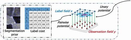
The CRF post-processing is independent of the network (Zhong et al. 2020). The introduced CRF model contains a unary potential term and a pairwise potential term (Zhong and Wang 2010). The CRF model is combined with the TERN model and label cost constraints to perform appropriate smoothing while considering the spatial-contextual information. In addition, in order to alleviate the effect of the within-class spectral variability and noise in the classification, a prior segmentation step is applied using the object-oriented strategy, to deal with the spatial heterogeneity issue. Finally, the optimal classification labels are obtained by the graph cut based α-expansion inference algorithm.

(i) Segmentation prior

The modelling of pairwise potentials depends on the accuracy of the probability estimation. LWIR hyperspectral images are severely disturbed by noise, and rely only on the network for feature extraction. There is also isolated pretzel noise, and the accuracy of the probability estimation still needs to be improved. In contrast, the object-oriented approach uses the segmented objects as the basic analysis units, which is an approach that can consider large-scale spatial-contextual information and has a good mitigation effect with regard to salt-and-pepper noise.

The segmentation result is obtained based on the classification graph using a connected region labelling algorithm, and the connected regions with the same labelling as the iterative classification graph are used as the segmentation regions. Thus, selection of the segmentation scale can be avoided. The classical eight-neighbourhood connected region labelling algorithm for data structure was utilized in the experiments to obtain the segmented objects [28]. Then, based on the classification graph of the TERN model, the labelling of each segmentation object can be obtained by the majority voting strategy, so that the segmentation prior is defined as:

(14) $P\left(x_i=l_{seg}\right)=max\left\{P\left(x_i=l_k\right),k\in \left|L\right|\right\}$(14)

where $l_{seg}$ represents the corresponding region label of the pixel.

(ii) Inference of CRF

Modelling the unary and pairwise potentials of LWIR hyperspectral images according to their characteristics requires an inference algorithm to predict the optimal category markers, which corresponds to finding the minimum of the energy function. Graph cuts is the most frequently used way to obtain the optimal markers. In this study, we used the graph cuts based α-expansion inference algorithm to obtain the optimal markers [28]. This algorithm is widely used in different fields and has an efficient inference capability. Figure 6 is a flowchart of partitioning the prior CRF.

Figure 6. Flowchart of the conditional random field model.

4. Experiments and analysis

The performance of the proposed TERN-CRF framework was investigated with three datasets: the mineral dataset, the tree leaves dataset, and the Dongguo Lake dataset. Also, to further validate the effectiveness of the proposed TERN-CRF method, the computational efficiency of all the methods was assessed, and an ablation study was performed to verify the effectiveness of the temperature-emissivity residual network and CRF model.

4.1. Experimental settings

In the three above-mentioned datasets, we randomly selected 100 pixels of every class for the training, and the remaining pixels were used for the testing. To be more specific, the total number of training pixels was only 2.63%, 3.04%, and 3.06% of all the labelled pixels for the mineral data, the tree leaves data and the Dongguo lake data, respectively. Tables 1–3 list the training and test information of the three LWIR datasets and the label setting is the same in all methods.

Table 1. Training and test samples of the mineral dataset.

No.	Class	Train	Test
1	Calcite	100	5260
2	Fibrous gypsum	100	5376
3	Anhydrite	100	4079
4	Dolomite	100	4418
5	Talc	100	2447
6	Diopside	100	3784
7	Concrete floor	100	537
	Total	700	25,901

Table 2. Training and test samples of the tree leaves dataset.

No.	Class	Train	Test
1	Photinia	100	3809
2	Evergreen magnolia	100	4981
3	Grass	100	1020
4	Camphor	100	3745
5	Osmanthus	100	3055
6	Mulberry	100	4483
7	Privet	100	1226
8	Concrete floor	100	3191
	Total	800	25,510

Table 3. Training and test samples of the Dongguo Lake dataset.

No.	Class	Train	Test
1	Building	100	122
2	Road	100	10,234
3	Sand	100	3783
4	Water	100	1929
5	Vegetation	100	2151
6	Bare soil	100	800
	Total	600	19,019

The proposed method was compared with both classical and deep learning methods: support vector machine (SVM) (Chang and Lin 2011), SVM-CRF (Zhong, Zhao, and Zhang 2014), FNEA-OO (Mallinis et al. 2008), HybridSN (Roy, Krishna, and Dubey 2019), AF_3DCNN (Ahmad, Khan and Mazzara et al. 2020), a CNN-based method (Du et al. 2019), and CNN-CRF (Zhong et al. 2020). For SVM, we adopted the spectral-based pixel-wise SVM classification algorithm in the LIBSVM package. The kernel of SVM was a radial basis function (RBF), and the penalty factor C was optimized through five-fold cross-validation. In order to introduce the spatial information of the LWIR hyperspectral images, we also compared object-oriented and CRF classification methods. The object-oriented classification (OOC) method was the multi-resolution segmentation algorithm in eCognition 8.0. The OOC results were obtained by performing a majority vote on each object, based on the classification map of pixel-by-pixel SVM. In order to determine the best segmentation scale, the experimental data were segmented according to the scale coefficient of 3–15, and the best classification results were selected as the final experimental results. We refer to this method as FNEA-OO. To demonstrate the advantages of the TERN model in classification, it was also compared with the baseline CNN network, HybridSN and AF_3DCNN. The latter two methods were specifically proposed for hyperspectral classification. Finally, the SVM-CRF, CNN-CRF, and TERN-CRF methods were compared with the SVM, CNN, and TERN methods, to show the advantages of combining the CRF classification framework with spatial-contextual information. The overall accuracy (OA), average accuracy (AA), and kappa coefficient (Kappa) are introduced to evaluate the accuracy of the classification results.

4.2. Results for the mineral dataset

The visual effect of the image classification map is an important way to evaluate classification methods. Figure 7 shows the quantitative results of the proposed TERN-CRF method and the other comparison methods obtained with the mineral dataset. For the result of SVM, because of the spectral similarity of the emissivity spectra of the different minerals, this method based on the spectral information of pixels shows obvious salt-and-pepper noise. At the same time, there are a lot of misclassified pixels in the mineral boundary areas. The other methods that consider the spatial information, i.e. SVM-CRF, FNEA-OO, HybridSN, AF_3D CNN, CNN-CRF, and TERN-CRF, show better visual classification results. This indicates that spatial information can be taken into account when classifying LWIR hyperspectral imagery, to reduce the salt-and-pepper noise and improve the classification accuracy. The FNEA-OO method obtains the smoothest classification image, but the result of the classification depends on the shape of the segmentation. In those methods considering spatial-contextual information, such as SVM-CRF, CNN-CRF and TERN-CRF, the salt-and-pepper noise is greatly reduced, with only a very small number of error regions. This proves that the CRF model can alleviate the salt-and-pepper noise problem in classifying LWIR hyperspectral images, regardless of whether a traditional classification method or a deep learning method is used.

Figure 7. The classification results for the mineral dataset.

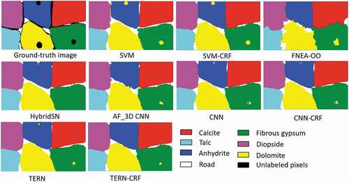
From another point of view, the quantitative evaluation of the classification results can better reflect the performance of the classification methods. The quantitative results of all the classification methods for the mineral dataset are listed in Table 4, where it can be seen that the quantitative results are similar to the visual results. Compared with pixel-based SVM, the OAs of SVM- CRF, HybridSN, AF_3D CNN, CNN, CNN-CRF, TERN, and TERN-CRF are improved by 0.44%, 0.41%, 0.29%, 0.61%, 0.63%, 0.67%, and 0.69%, respectively, and the OA of FNEA-OO is 2.64% lower than that of SVM. This demonstrates the effectiveness of incorporating spatial information, but due to the FNEA-OO method relying on accurate segmentation results, it is not suitable for Fourier- transformed LWIR hyperspectral images. The proposed TERN-CRF method obtains the best OA, AA, and Kappa values. Because of the simple distribution of the mineral scene and the large spectral differences between the different minerals, the pixel-based method can obtain good classification results. Compared with SVM, CNN, and TERN, the SVM-CRF, CNN-CRF, and TERN-CRF methods obtain slightly improved classification accuracies, which, to some extent, indicates the effectiveness of the CRF model. Although combining the deep learning methods with CRF can improve the accuracy of the classification, the effect is not obvious.

Table 4. Classification results of the different methods for the mineral dataset.

	SVM	SVM-CRF	FNEA-OO	Hybrid-SN	AF_3D CNN	CNN	CNN- CRF	TERN	TERN-CRF
OA(%)	99.05	99.49	96.41	99.46	99.34	99.66	99.68	99.72	99.74
AA(%)	99.12	99.56	92.54	99.21	98.46	99.34	99.39	99.38	99.45
Kappa	0.99	0.99	0.96	0.99	0.99	0.99	0.99	0.99	0.99
Calcite	99.41	99.68	97.45	99.87	99.98	99.81	99.83	99.85	99.90
Fibrous gypsum	98.85	99.22	96.28	99.27	99.46	99.94	99.94	99.57	99.55
Anhydrite	98.45	98.79	95.98	99.41	98.84	99.85	99.88	99.93	99.88
Dolomite	99.12	99.55	96.72	98.87	99.27	99.19	99.39	99.80	99.59
Talc	98.36	99.89	98.04	99.96	99.14	99.18	100	99.55	99.97
Diopside	99.68	100.00	98.68	99.89	99.94	100	97.58	99.95	97.39
Concrete floor	100	100	64.62	97.21	92.55	97.39	97.58	97.02	97.39

4.3. Results for the tree leaves dataset

Figure 8 shows the classification results of the different methods for the tree leaves dataset. The spectral-based SVM classifier shows a large amount of salt-and-pepper noise and staggered pixels in the results. SVM-CRF, HybridSN, AF-3D CNN, CNN, CNN-CRF, TERN, and TERN-CRF obtain smoother classification results by considering the spatial neighbourhood information.

Figure 8. The classification results for the tree leaves dataset.

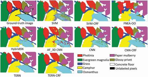
Table 5 provides the corresponding quantitative evaluation results. Compared with SVM, the OAs of these methods are increased by 11.53%, 11.67%, 8.94%, 9%, 11.35%, 14.44%, and 14.95%, respectively. For the object-oriented method, the accuracy of the segmentation directly determines the accuracy of the classification. However, because of the complexity of the tree leaves dataset, it is difficult to determine the optimal segmentation scale. Although the FNEA-OO classification results are smooth and the OA value of the classification is increased by 9%, there is a lot of misclassification at the edges of the leaves, and the edge contours do not agree with the shapes of the leaves. The CNN method can extract the deep information in the LWIR imagery, and the result is better than that of the traditional pixel-based SVM and object-oriented FNEA-OO classification methods. However, the result still contains a large number of isolated misclassification regions, and the edges are badly mixed. The same situation occurs in HybridSN and AF_3D CNN, although both utilizes spatial-spectral feature. The classification map obtained by the TERN method is smoother than that obtained by the CNN method, and the number of isolated regions is reduced. The salt-and-pepper noise and isolated staggered regions in the SVM, CNN, and TERN results are improved by adding the CRF model with spatial-contextual information. The OA is also improved by 11.53%, 2.37%, and 0.51%, respectively. The proposed TERN-CRF method achieves the best OA, AA, and Kappa values on the tree leaves dataset.

Table 5. Classification results of the different methods for the tree leaves dataset.

	SVM	SVM-CRF	FNEA-OO	Hybrid-SN	AF_3D CNN	CNN	CNN- CRF	TERN	TERN-CRF
OA(%)	83.32	94.85	85.24	94.99	92.26	92.32	94.67	97.76	98.27
AA(%)	80.60	93.53	79.77	94.32	90.39	90.03	92.99	97.21	98.01
Kappa	0.81	0.94	0.83	094	0.91	0.91	0.94	0.97	0.98
Photinia	84.30	95.21	89.44	96.10	94.39	97.13	97.55	98.55	98.79
Evergreen magnolia	93.94	95.84	94.88	95.48	96.58	97.11	97.17	97.37	97.39
Grass	85.78	94.61	63.92	91.27	89.50	91.76	93.82	95.59	95.59
Camphor	80.88	89.05	86.65	94.02	93.21	89.48	91.11	98.56	99.57
Osmanthus	56.04	97.84	84.98	95.19	80.52	83.18	94.40	98.76	99.38
Paper mulberry	87.66	98.53	91.97	96.72	96.07	95.27	96.25	97.75	98.53
Glossy privet	59.30	79.61	52.61	92.01	79.28	70.80	76.92	92.99	97.63
Concrete floor	96.90	97.56	73.68	93.73	93.60	95.49	96.68	98.09	97.18

4.4. Results for the Dongguo Lake dataset

Figure 9 shows the visual results of the different classification methods for the aerial Dongguo Lake dataset. For SVM and CNN that only consider spectral information, the classification results still suffer from spatial noise. For other methods considering spatial features, the classification results have better performance than the above two methods in terms of spatial consistency. Since the study area is a park, vegetation and bare soil are interspersed, and those are easy to misclassify.

Figure 9. The classification results for the Dongguo Lake dataset.

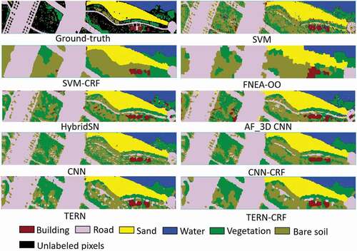
Table 6 lists the corresponding quantitative evaluation results, and the classification accuracy of all deep learning methods are higher than 90% except for CNN. The SVM method obtains an 82.17% OA value, and the classification accuracy for vegetation and bare soil is only 64.30% and 60.50%. Compared with SVM, the OA of SVM-CRF is 2.49% higher, and the isolated regions and salt-and-pepper noise are improved. The OA of FNEA-OO is 2.49% higher than that of SVM, but the original fragmented vegetation and bare soil areas are all classified as smooth blocks in this complex natural scene. It is difficult to obtain a good segmentation result with a single segmentation scale, which leads to the poor visualization of the classification results. The CNN methods achieve improvements of 6.89% in OA compared with SVM, which shows the ability of deep learning algorithms to extract deep features in complex scenes. The Hybrid-SN, AF_3D CNN, CNN-CRF, TERN and TERN_CRF method also solves the problem of broken areas, and the OA of those above methods are higher than 90%. Compared with Hybrid-SN, AF_3D CNN, the classification accuracy of TERN therefore proves the ability of the residual network to extract deep spatial and spectral features. The classification result obtained by TERN is 93.95%, which is higher than 90.80% and 90.67% of HybridSN and AF_3D CNN. Compared with TERN, TERN-CRF achieves a better classification result with CRF model as a post-process procedure. Analysed from another perspective, the OA of the SVM-CRF, CNN-CRF, and TERN-CRF methods is improved by 2.49%, 2.66%, and 0.47% over their baseline methods, respectively.

Table 6. Classification results of the different methods for the Dongguo Lake dataset.

	SVM	SVM-CRF	FNEA-OO	Hybrid- SN	AF_3D CNN	CNN	CNN- CRF	TERN	TERN-CRF
OA(%)	82.17	84.66	86.56	90.80	90.67	89.06	91.72	93.95	94.42
AA(%)	80.36	83.25	82.22	89.23	90.11	86.19	89.65	89.58	89.59
Kappa	0.74	0.78	0.80	0.86	0.86	0.84	0.88	0.91	0.92
Building	87.70	97.54	89.34	94.26	98.36	98.36	98.36	98.36	96.72
Road	80.67	87.18	88.09	90.00	89.05	89.41	91.27	95.55	95.99
Sand	94.45	97.65	96.83	98.33	99.28	98.68	99.37	99.50	99.42
Water	94.56	97.25	91.50	98.60	98.49	97.77	98.60	99.90	99.95
Vegetation	64.30	39.38	65.83	80.57	82.24	73.04	82.94	83.31	86.19
Bare soil	60.50	80.50	61.75	73.63	73.25	59.88	67.38	60.88	59.25

4.5. Computational Efficiency

The computational efficiency of the different classification methods was analysed using the mineral dataset, tree leaves dataset, and Dongguo Lake dataset. The SVM, FNEA-OO, and SVM-CRF methods were implemented in MATLAB 2016 and eCognition 8.0 on a laptop computer equipped with an Intel Core i5 -10,210 U CPU. The CNN and CNN-CRF methods were implemented in the TensorFlow toolbox and MATLAB 2016 under CUDA 9 with an NVIDIA GeForce RTX 2080 Ti GPU and an Intel Core i5 -10,210 U CPU. The TERN and TERN-CRF models had the same configuration as the CNN and CNN-CRF models.

Table 7 lists the average running times of the different classification methods for the three datasets. In this experiment, the probability images obtained by the SVM, CNN, and TERN methods were used as the unary potential terms of the SVM-CRF, CNN-CRF and TERN-CRF methods, respectively. Therefore, the training times of the SVM-CRF, CNN-CRF, and TERN-CRF methods were the same as those of the SVM, CNN, and TERN methods. The results for the three datasets illustrate that the speed of the model is reduced after adding the CRF model. Since deep learning requires a long time for sample training, the deep learning based methods take more time than SVM, SVM-CRF, and FNEA-OO. The training and testing time of HybirdSN, AF_3D CNN, CNN, CNN-CRF is less than TERN and TERN-CRF. In the test process, the test times of SVM, SVM-CRF, and FNEA-OO are close to the training times, and the test time increases significantly as the image size increases. In contrast, the deep learning test time does not increase by much, and the test time of TERN-CRF is only about 10% of the training time for these three datasets, which is lower than that of CNN-CRF, HybirdSN and AF_3D CNN.

Table 7. Average running times for the different classification methods. Time: s.

Dataset		SVM	SVM-CRF	FNEA-OO	Hybrid -SN	AF_3D CNN	CNN	CNN-CRF	TERN	TERN-CRF
Mine-ral	Training	3.54	3.54	6.31	58.08	64.20	32.46	32.46	562.22	562.22
	Test	2.15	4.18	2.78	19.67	16.26	4.26	6.12	50.82	52.63
Tree leaves	Training	3.21	3.21	6.53	55.09	71.49	33.46	33.46	559.87	559.87
	Test	2.33	5.01	2.54	17.53	15.53	4.79	7.55	52.32	53.87
Dongguo Lake	Training	5.19	5.19	14.03	65.90	58.23	56.11	56.11	775.65	775.65
	Test	3.58	7.23	3.93	13.02	12.27	8.51	10.09	84.18	86.18

5. Discussion

5.1. Residual network and CRF advantage analysis

To analyse the advantage of the residual network and CRF model, the classification results for a novel Fourier-transformed LWIR hyperspectral data between the baseline network CNN and TERN, as well as the results before and after the addition of the CRF model are discussed.

The comparison of the classification results of CNN and TERN in Figures 8 and 9 demonstrate that CNN has more misclassifications. For example, a part of privet is misclassified as Osmanthus in Figure 8 because of the similarity of spectra as shown in Figure 3(e). In the classification maps of Dongguo Lake dataset, the road is also incorrectly classified seriously of CNN method. Adding residual network can effectively improve the classification results and alleviate the misclassifications. However, although TERN can effectively solve the problems of spectral similarity and partial spatial consistency, there are still holes and isolated areas in the classification results, such as the edge of leaves in Figure 8. CRF with the temperature image utilizes spatial context information to eliminate these isolated regions as shown in Figures 8 and 9. Both CNN and TERN adding the CRF post-processing, the isolated misclassification area is significantly reduced.

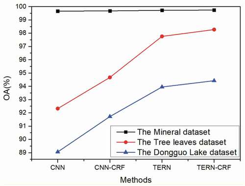
Figure 10 is a comparison of quantitative results obtained by the CNN, CNN-CRF, TERN, and TERN-CRF methods for the three datasets. To make a fair comparison, we set the same input volume size of 7 × 7 × b for all the methods, and adjusted these other methods to their optimal settings. Since the distribution of the mineral dataset is simple and obvious, the classification accuracies of all the methods show little difference, and the methods all obtain an accuracy of higher than 99%. For the tree leaves dataset and the Dongguo Lake dataset, the TERN method achieves a nearly 5% accuracy improvement over the benchmark CNN method. It deduces that the temperature-emissivity residual network can extract and fuse in-depth spectral and spatial features. After adding the CRF model, the accuracies of the CNN and TERN methods are significantly improved. The CRF model further incorporates the spatial-contextual information in the classification map to reduce small isolate areas. Among all the methods, the proposed TERN-CRF method performs the best of all.

Figure 10. Comparison of the classification accuracies of the CNN, CNN-CRF, TERN, and TERN-CRF methods for the three datasets.

5.2. Limitations of this study

Although the spatial and spatial residual network and the CRF model can improve the accuracy of classification for two filed and one aerial LWIR hyperspectral images, the classification results are limited by the distribution of land surface and the richness types of features. In addition, the sum of training and testing time of TERN-CRF will increase with the increase of image size. Therefore, our future research work will pay attention to the practical application of rich ground object types and large-scale precise classification, and more efficient and advanced classifiers, such as the fast patch-free global learning (FPGA) (Zheng et al. 2020), the spectral patching network (SPNet) (Hu et al. 2021), will be tried in LWIR image classification.

6. Conclusions

In this paper, aiming at the problems of the high spectral similarity and spatial heterogeneity in the classification of Fourier-transformed LWIR hyperspectral images, the TERN-CRF classification method based on temperature and emissivity information for Fourier-transformed LWIR hyperspectral imagery has been proposed. Three LWIR datasets (two field-based datasets and one aerial dataset) were built in this study. The classification results obtained with these datasets demonstrated that the proposed TERN-CRF method for the classification of LWIR hyperspectral imagery has obvious advantages over the traditional SVM and object-oriented FNEA-OO methods, and the residual network has certain advantages over a CNN network, HybridSN and AF_3DCNN. In addition, the CRF model can improve the problem of holes and isolated regions in the classification map. Larger scenes and efficient classifiers are being implemented in future studies in order to increase the classification application of LWIR hyperspectral imagery.

Disclosure statement

No potential conflict of interest was reported by the author(s).

Additional information

Funding

This research was funded in part by the National Key Research and Development Program of China under grant 2021YFE0117100, in part by the National Natural Science Foundation of China under grants 41771385 and 42071350.

References

- Adler-Golden, S. M., P. Conforti, M. Gagnon, P. Tremblay, and M. Chamberland. 2014. Long-Wave Infrared Surface Reflectance Spectra Retrieved from Telops Hyper-Cam Imagery In Proceeding of SPIE, Algorithms & Technologies for Multispectral, Hyperspectral, & Ultraspectral Imagery XX. Baltimore, Maryland, United States: International Society for Optics and Photonics. 13 th July, Vol. 9088. doi:10.1117/12.2050446
- Ahmad, M., A.M. Khan, M. Mazzara, et al. 2020. ”A Fast and Compact 3-D CNN for Hyperspectral Image Classification.” IEEE Geoscience and Remote Sensing Letters 19 (5502205): 1–5. doi:10.1109/LGRS.2020.3043710.
- Aslett, Z., J. V. Taranik, and D. N. Riley. 2017. “Mapping Rock Forming Minerals at Boundary Canyon, Death Valley National Park, California, Using Aerial SEBASS Thermal Infrared Hyperspectral Image Data.” International Journal of Applied Earth Observation and Geoinformation 64: 326–339. doi:10.1016/j.jag.2017.08.001.
- Barisione, F., D. Solarna, A. D. Giorgi, G. Moser, and S. B. Serpico 2016. “Supervised Classification of Thermal Infrared Hyperspectral Images Through Bayesian, Markovian, and Region-Based Approaches.” in 2016 IEEE International Geoscience and Remote Sensing Symposium (IGARSS), Beijing, China, July 10-15. doi: 10.1109/IGARSS.2016.7729237
- Cao, G., L. Zhou, and Y. Li. 2016. “A New Change-Detection Method in High-Resolution Remote Sensing Images Based on a Conditional Random Field Model.” International Journal of Remote Sensing 37 (5–6): 1173–1189. doi:10.1080/01431161.2016.1148284.
- Chang, C.-C. and C.-J. Lin. 2011. “LIBSVM: A Library for Support Vector Machines.” ACM Transactions on Intelligent Systems and Technology (TIST) 2 (3): 1–27. doi:10.1145/1961189.1961199.
- Chen, Y., H. Jiang, C. Li, X. Jia, and P. Ghamisi. 2016. “Deep Feature Extraction and Classification of Hyperspectral Images Based on Convolutional Neural Networks.” IEEE Transactions on Geoscience and Remote Sensing 54 (10): 6232–6251. doi:10.1109/TGRS.2016.2584107.
- Du, P., E. Li, J. Xia, A. Samat, and X. Bai. 2019. “Feature and Model Level Fusion of Pretrained CNN for Remote Sensing Scene Classification.” IEEE Journal of Selected Topics in Applied Earth Observations and Remote Sensing 12 (8): 2600–2611. doi:10.1145/1961189.1961199.
- Harrison, D., B. Rivard, and A. Sánchez-Azofeifa. 2018. “Classification of Tree Species Based on Longwave Hyperspectral Data from Leaves, a Case Study for a Tropical Dry Forest.” International Journal of Applied Earth Observation and Geoinformation 66: 93–105. doi:10.1016/j.jag.2017.11.009.
- He, K., X. Zhang, S. Ren, and J. Sun 2016. “Deep Residual Learning for Image Recognition.” Proceedings of the IEEE Conference on Computer Vision and Pattern Recognition, Las Vegas, NV, USA, 27-30 June, 770–778. arXiv:1512.03385
- Hu, X., Y. Zhong, X. Wang, C. Luo, and L. Zhang. 2021. “Spnet: Spectral Patching End-To-End Classification Network for UAV-Borne Hyperspectral Imagery with High Spatial and Spectral Resolutions.” IEEE Transactions on Geoscience and Remote Sensing 99: 1–17. doi:10.1109/TGRS.2020.2967821.
- Hunt, G. R. 2012. “Spectral Signatures of Particulate Minerals in the Visible and Near Infrared.” Geophysics 42 (3): 501–513. doi:10.1190/1.1440721.
- Iqbal, A., S. Ullah, N. Khalid, W. Ahmad, I. Ahmad, M. Shafique, G. C. Hulley, D. A. Roberts, and A. K. Skidmore. 2018. “Selection of HyspIri Optimal Band Positions for the Earth Compositional Mapping Using HyTes Data.” Remote Sensing of Environment 206: 350–362. doi:10.1016/j.rse.2017.12.005.
- Kirkland, L., K. Herr, E. Keim, P. Adams, J. Salisbury, J. Hackwell, and A. Treiman. 2002. “First Use of an Airborne Thermal Infrared Hyperspectral Scanner for Compositional Mapping.” Remote Sensing of Environment 80 (3): 447–459. doi:10.1016/S0034-4257(01)00323-6.
- Liu, C., R. Xu, F. Xie, J. Jin, L. Yuan, G. Lv, Y. Wang, C. Li, and J. Wang. 2020. “New Airborne Thermal-Infrared Hyperspectral Imager System: Initial Validation.” IEEE Journal of Selected Topics in Applied Earth Observations and Remote Sensing 13: 4149–4165. doi:10.1109/JSTARS.2020.3010092.
- Luz, B. R. D. and J. K. Crowley. 2007. “Spectral Reflectance and Emissivity Features of Broad Leaf Plants: Prospects for Remote Sensing in the Thermal Infrared (8.0–14.0 μm).” Remote Sensing of Environment 109 (4): 393–405. doi:10.1016/j.rse.2007.01.008.
- Mallinis, G., N. Koutsias, M. Tsakiri-Strati, and M. Karteris. 2008. “Object-Based Classification Using Quickbird Imagery for Delineating Forest Vegetation Polygons in a Mediterranean Test Site.” ISPRS Journal of Photogrammetry and Remote Sensing 63: 237–250. doi:10.1016/j.isprsjprs.2007.08.007.
- Manolakis, D., M. Pieper, E. Truslow, R. Lockwood, and T. Cooley. 2019. “Longwave Infrared Hyperspectral Imaging: Principles, Progress, and Challenges.” IEEE Geoscience and Remote Sensing Magazine 7 (2): 72–100. doi:10.1109/MGRS.2018.2889610.
- Marwaha, R., A. Kumar, and A. S. Kumar. 2015. “Object-Oriented and Pixel-Based Classification Approach for Land Cover Using Airborne Long-Wave Infrared Hyperspectral Data.” Journal of Applied Remote Sensing 9 (1): 1–20. doi:10.1117/1.JRS.9.095040.
- Pan, B., Z. Shi, and X. Xu. 2017. “Longwave Infrared Hyperspectral Image Classification via an Ensemble Method.” International Journal of Remote Sensing 38 (22): 6164–6178. doi:10.1080/01431161.2017.1348643.
- Reynolds, J. and K. Murphy 2007. “Figure-Ground Segmentation Using a Hierarchical Conditional Random Field.” Fourth Canadian Conference on Computer and Robot Vision (CRV’07), Montreal, QC, Canada, 28-30 May, 2007, 175–182.
- Rivard, B. and G. A. Sánchez-Azofeifa. 2018. “Discrimination of Liana and Tree Leaves from a Neotropical Dry Forest Using Visible-Near Infrared and Longwave Infrared Reflectance Spectra.” Remote Sensing of Environment 219: 135–144. doi:10.1016/j.rse.2018.10.014.
- Rock, G., M. Gerhards, M. Schlerf, C. Hecker, and T. Udelhoven. 2016. “Plant Species Discrimination Using Emissive Thermal Infrared Imaging Spectroscopy.” International Journal of Applied Earth Observation & Geoinformation 53: 16–26. doi:10.1016/j.jag.2016.08.005.
- Roy S. K., G. Krishna, and S. R. Dubey, et al. 2019. ”HybridSn: Exploring 3-D–2-D CNN Feature Hierarchy for Hyperspectral Image Classification.” IEEE Geoscience and Remote Sensing Letters 17 (2): 277–281. doi:10.1109/LGRS.2019.2918719.
- Sminchisescu, C., A. Kanaujia, and D. Metaxas. 2006. “Conditional Models for Contextual Human Motion recognition.” Computer Vision and Image Understanding 104 (2–3): 210–220. doi:10.1016/j.cviu.2006.07.014.
- Ullah, S., M. Schlerf, A. K. Skidmore, and C. Hecker. 2012. “Identifying Plant Species Using Mid-Wave Infrared (2.5–6 μm) and Thermal Infrared (8–14 μm) Emissivity Spectra.” Remote Sensing of Environment 118: 95–102. doi:10.1016/j.rse.2011.11.008.
- Vaughan, R. G., W. M. Calvin, and J. V. Taranik. 2003. “SEBASS Hyperspectral Thermal Infrared Data: Surface Emissivity Measurement and Mineral Mapping.” Remote Sensing of Environment 85 (1): 48–63. doi:10.1016/S0034-4257(02)00186-4.
- Vaughan, R. G., S. J. Hook, W. M. Calvin, and J. V. Taranik. 2005. “Surface Mineral Mapping at Steamboat Springs, Nevada, USA, with Multi-Wavelength Thermal Infrared Images.” Remote Sensing of Environment 99 (1–2): 140–158. doi:10.1016/j.rse.2005.04.030.
- Weksler, S., O. Rozenstein, and E. Ben-Dor. 2018. “Mapping Surface Quartz Content in Sand Dunes Covered by Biological Soil Crusts Using Airborne Hyperspectral Images in the Longwave Infrared Region.” Minerals 8 (8): 318–331. doi:10.3390/min8080318.
- Yang, X., Y. Ye, X. Li, R. Y. K. Lau, X. Zhang, and X. Huang. 2018. “Hyperspectral Image Classification with Deep Learning Models.” IEEE Transactions on Geoscience and Remote Sensing 56 (9): 5408–5423. doi:10.1109/TGRS.2018.2815613.
- Zhao, J., Y. Zhong, and L. Zhang. 2015. “Detail-Preserving Smoothing Classifier Based on Conditional Random Fields for High Spatial Resolution Remote Sensing Imagery.” IEEE Transactions on Geoscience and Remote Sensing 53 (5): 2440–2452. doi:10.1109/TGRS.2014.2360100.
- Zheng, Z., Y. Zhong, A. Ma, and L. Zhang. 2020. “FPGA: Fast Patch-Free Global Learning Framework for Fully End-To-End Hyperspectral Image Classification.” IEEE Transactions on Geoscience and Remote Sensing 58 (8): 5612–5626. doi:10.1109/TGRS.2020.2967821.
- Zhong, Y., X. Hu, C. Luo, X. Wang, J. Zhao, and L. Zhang. 2020. “WHU-Hi: UAV-Borne Hyperspectral with High Spatial Resolution (H2) Benchmark Datasets and Classifier for Precise Crop Identification Based on Deep Convolutional Neural Network with CRF.” Remote Sensing of Environment 250 (1): 112012. doi:10.1016/j.rse.2020.112012.
- Zhong, Z., J. Li, D. A. Clausi, and A. Wong. 2020. “Generative Adversarial Networks and Conditional Random Fields for Hyperspectral Image Classification.” IEEE Transactions on Cybernetics 50 (7): 3318–3329. doi:10.1109/TCYB.2019.2915094.
- Zhong, Z., J. Li, Z. Luo, and M. Chapman. 2018. “Spectral–spatial Residual Network for Hyperspectral Image Classification: A 3-D Deep Learning Framework.” IEEE Transactions on Geoscience and Remote Sensing 56 (2): 847–858. doi:10.1109/TGRS.2017.2755542.
- Zhong, P. and R. Wang. 2010. “Learning Conditional Random Fields for Classification of Hyperspectral Images.” IEEE Transactions on Image Processing 19 (7): 1890–1907. doi:10.1109/TIP.2010.2045034.
- Zhong, Y., J. Zhao, and L. Zhang. 2014. “A Hybrid Object-Oriented Conditional Random Field Classification Framework for High Spatial Resolution Remote Sensing Imagery.” IEEE Transactions on Geoscience and Remote Sensing 52 (11): 7023–7037. doi:10.1109/TGRS.2014.2306692.
- Zhu, X., L. Cao, S. Wang, L. Gao, and Y. Zhong. 2021. “Anomaly Detection in Airborne Fourier Transform Thermal Infrared Spectrometer Images Based on Emissivity and a Segmented Low-Rank Prior.” Remote Sensing 13 (4): 754–775. doi:10.3390/rs13040754.