
 ?Mathematical formulae have been encoded as MathML and are displayed in this HTML version using MathJax in order to improve their display. Uncheck the box to turn MathJax off. This feature requires Javascript. Click on a formula to zoom.
ABSTRACT
The Eastern Mediterranean Sea has been known as an oil pollution hotspot due to its heavy marine traffic and an increasing number of oil and gas exploration activities. To provide automatic detection of oil pollution from not only maritime accidents but also deliberate discharges in this region, a deep learning-based object detector was developed utilizing freely available Sentinel-1 Synthetic Aperture Radar (SAR) imagery. A total of 9768 oil objects were collected from 5930 Sentinel-1 scenes from 2015 to 2018 and used for training and validating the object detector and evaluating its performance. The trained object detector has an average precision (AP) of 69.10% and 68.69% on the validation and test sets, respectively, and it could be applied for building an early-stage oil contamination surveillance system.
1. Introduction
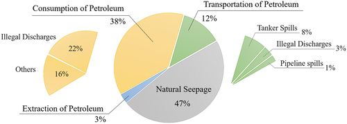
Marine oil pollution has long been a serious problem for the maritime environment. Sources of oil pollution can be categorized into several groups: natural seepage, consumption of petroleum, transportation of petroleum and extraction of petroleum. shows the global average contributions of sources in marine waters for the years of 1975–1985 and 1990–1999 (Polinov, Bookman and Levin Citation2021). Most of the large oil spills come from tanker accidents, however they cover only around 8% of the total oil pollution. Illegal discharges, such as the release of oily ballast water, tanker washing residue, fuel oil sludge, engine waste and foul bilge water, account for the majority of human-caused oil pollution. Large oil spills in particular pose a great risk of environmental damage, but deliberate illegal discharges pose a constant threat to marine wildlife with potentially severe long-term consequences. The inhalation of volatile petroleum by mammals and birds at sea can cause irritation to their respiratory tract and narcosis (Saadoun Citation2015). Oil spill detection is therefore important not only for those maritime accidents, but also for tracking deliberate oil pollution.
Figure 1. Main sources of petroleum entering worldwide marine waters with their average contributions for the years of 1975–1985 and 1990–1999 (Polinov, Bookman and Levin Citation2021).
Marine oil pollution ‘hotspots’ usually coincide with areas of high maritime traffic (Polinov, Bookman and Levin Citation2021). Offering the shortest shipping route from Asia to Europe, approximately 30% of all international merchant vessels pass through the Mediterranean Sea (REMPEC Citation2002). The Mediterranean Sea is also an important oil transit centre for transporting crude oil from the Middle East, North Africa and the Black Sea to Europe and North America. Around 20% to 25% of the world’s oil tankers transit the Mediterranean Sea (REMPEC Citation2002). A previous study showed that the frequent oil spills in this area are usually related to shipping routes, oil terminals and transboundary shipping ports (Abdulla and Linden Citation2008). After the discovery of natural gas and oil in the Levantine basin in late 2010, there has been an increase in offshore oil and gas exploration and exploitation activities in the Eastern Mediterranean Sea. The Levantine region has thus become known as an oil spill hotspot. The situation is exacerbated by a lack of oversight due to the regional political instability (Polinov, Bookman and Levin Citation2021). One such oil spill event, which seriously influenced the coastline of Israel, was reported on 17 February 2021, but it could actually have already been found on satellite images on 11 February (Surkes, 28 February 2021). This and other events highlight the importance of having a reliable surveillance system for locating oil spills in the early stages in order to support the clean-up operations.
With the advantage of wide coverage and the capability of monitoring at night and during cloudy weather, spaceborne Synthetic Aperture Radar (SAR) is suitable for setting up such an early warning system. Water surface roughness is a key factor for the radar sensor to receive enough backscattered microwave energy. Small wind-induced friction between the air and the water surface causes gravity-capillary waves in the range of millimetres to centimetres (Woodhouse Citation2006). Oil spills dampen these waves and thus reduce radar backscatter, resulting in dark formations in contrast to the surrounding spill-free sea surface (Pavlakis, Tarchi and Sieber Citation2001). However, there are many other phenomena, which can also manifest as dark regions in the radar image, such as low wind areas, natural films, wave fronts, wind sheltering by land, rain cells, wave current interaction along shears, internal waves, upwelling and eddies (Hovland, Johannessen and Digranes Citation1994; Topouzelis Citation2008). Distinguishing oil spills from these ‘look-alikes’ has long been a challenging task for oil spill detection with SAR.
The general procedure of detecting oil spills includes dark spot segmentation, feature extraction and classification (Solberg and Solberg Citation1996). Dark formations on SAR imagery are first separated from their surroundings. The features of each dark spot are then extracted and used to identify the differences between oil spills and look-alikes. Commonly used features are statistical, geometric, textural, contextual and SAR polarimetric characteristics (Al-Ruzouq et al. Citation2020). The exploitation of polarimetric features, such as standard deviation of co-polarization phase difference, entropy, geometric intensity, co-polarization power ratio and polarization span, seem to be beneficial (Solberg Citation2012; Singha et al. Citation2016); however, the unavailability of quad-pol or dual-pol acquisitions on a regular basis and the limited swath of those images make it hard to be applied in an operational system. With all the extracted features, the dark spots are finally classified using a probabilistic approach as possible oil spills or look-alikes (Solberg et al. Citation1999; Fiscella et al. Citation2000). Depending on the present local sea state, oil spill composition, age of oil spill, image resolution and incidence angle of the acquisition, the backscatter properties of oil spills vary (Topouzelis Citation2008). Thus, machine learning algorithms are introduced to solve this challenging classification problem. Machine learning algorithms learn the relationships between the features given by previous experiences and the class (i.e. oil spill or look-alike) of each dark spot. The most commonly applied machine learning algorithms for oil spill detection are decision tree (Topouzelis and Psyllos Citation2012), support vector machine (SVM) (Brekke and Solberg Citation2008) and artificial neural network (ANN) (Singha, Bellerby and Trieschmann Citation2013). Deep learning is also considered as a subset of machine learning techniques. Unlike traditional machine learning algorithms, which rely on predefined features, deep learning algorithms learn directly from the data. Deep learning networks contain many layers, which are capable of constructing a hierarchy of features to increase the complexity. As deep learning is completely data driven, it requires large amounts of data for training. In the past, most of the spaceborne SAR data was acquired for oil spill detection when there were known marine accidents. However, with the advent of the Sentinel-1 mission by the European Space Agency (ESA) launched in 2014, it is now possible to detect oil spills from different sources on a regular basis with its frequent acquisitions. With the increasing volume of accessible SAR data and improvements in computational power, deep learning algorithms have been applied in oil spill detection as well.
Some studies applied U-Net to classify each pixel into a different class, such as oil spill, look-alike, ship, land and sea (Shaban et al. Citation2021) or simply oil spill and sea (Ronci et al. Citation2020). U-Net follows an encoder-decoder architecture, where the encoder gradually extracts features from low-level details to high-level information as it becomes deeper, and the decoder propagates information back to the original image dimension. As the encoder-decoder structure helps capture features at different scales, several architectures have been applied on image segmentation. DeepLabv3+ outperformed the other deep convolutional neural network (DCNN) models, U-Net, LinkNet, PSPNet and DeepLabv2, with its improvements in producing distinctive object boundaries (Krestenitis et al. Citation2019). Adapting the network from DeepLabv3+, an improved version was carried out and achieved better capability for multi-scale targets (Ma et al. Citation2022). Another study presented CBD-Net; it includes spatial and channel squeeze excitation, which collects contextual information and enhances the network’s ability to distinguish boundary details. With this optimization, CBD-Net showed better completeness and correctness than U-Net, D-LinkNet and DeepLabv3 (Zhu et al. Citation2022). For applying deep learning-based methods, the preparation of a labelled dataset is usually the most time-consuming work, especially for training pixel-based classifiers, which require a pixel-based mask of different classes. Therefore, there were only 35 and 21 SAR scenes used in Ma et al. (Citation2022) and Zhu et al. (Citation2022), respectively.
Object detectors on the other hand can only provide a detection of oil spills at a target level, but the dataset labelling work is less complex for each image, which means a larger dataset can be compiled in the same amount of time. Thus, more oil spills from different sources and of different types and sizes could be included, which might result in a higher ability to detect not only maritime accidents but also regular deliberate oil pollution. A previous study investigated a two-stage CNN to perform an initial coarse detection of objects, and based on that applied a precise pixel-wise detection on side-looking airborne radar (SLAR) imagery (Nieto-Hidalgo et al. Citation2018). The study pointed out the feasibility of detecting oil spills with object detection algorithms. Two other studies applied Mask-region-based convolutional neural network (Mask-RCNN) and used a total of around 2000–3000 images (Emna et al. Citation2020; Yekeen and Balogun Citation2020). Mask-RCNN can be regarded as a combination of object detection and semantic segmentation, as it first detects objects along with their classes and further segments objects into masks. However, to build a near real-time (NRT) oil spill detection system, highly efficient one-stage object detection algorithms such as You Only Look Once (YOLO) may be considered to keep the processing latency at a minimum. Following the idea that humans can easily recognize objects in an image at a glance, the YOLO object detection algorithm only looks at an entire image once to detect all objects inside along with their class probabilities (Redmon et al. Citation2016). It has been used in ship detection with SAR images in previous studies (Chang et al. Citation2019; Devadharshini et al. Citation2020), and one other study applied it on oil spill detection with optical imagery (Ghorbani and Behzadan Citation2021). However, applying YOLO on oil spill detection with SAR imagery is presented for the first time in this study.
This study developed a deep learning-based oil spill detector for the Eastern Mediterranean Sea using the YOLOv4 object detection algorithm. The object detector was trained with a total of 5930 Sentinel-1 images from 2015 to 2018, including 9768 oil spills from different sources and with different sizes collected and labelled as oil objects. With the use of such a large dataset, the capability of detecting deliberate oil spills is highlighted. CleanSeaNet is an existing service provided by the European Maritime Safety Agency (EMSA) using spaceborne SAR data to detect possible oil spills on the sea surface in European waters and sending oil spill alerts to national authorities (European Maritime Safety Agency Citation2017), but it is highly reliant on manual inspection, which is costly and time consuming. Therefore, this study aims to develop a deep learning-based oil spill detector for setting up an early-stage surveillance system. Different scenarios are carried out for training the object detector, and the detection results are discussed in the following sections.
The paper first introduces the used data and methods in section 2. Detailed information about the acquired SAR images is shown in subsection 2.1. Collecting oil spills and procedures of building the dataset are explained in subsections 2.2 and 2.3, respectively. The deep learning-based object detection algorithm YOLOv4 is introduced in subsection 2.4. Subsections 3.1 and 3.2 describe different scenarios for training the object detector. A further improved trained model and examples of detections are provided in subsection 3.3; the subsection also includes a comparison between the YOLOv4 custom trained model with one trained with another object detection algorithm, Faster RCNN. Section 4 summarizes the findings in this study.
2. Methodology
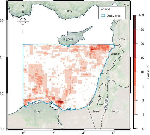
Oil spills in different areas might have varying patterns due to different origins, meteorological conditions, currents and circulation systems. This study focused on oil spills in the Eastern Mediterranean Sea, between longitudes 30–36°E and latitudes 31–34.7°N. The enclosed area with blue outline in shows the location of the study area, together with the number of collected oil spills between 2015 and 2018.
Figure 2. Visualization of study area with heat map of the amount of oil spills collected inside. The blue outline marks the study area. The red color map shows numbers of oil spills collected and manually annotated in this study from 2015 to 2018; see subsection 2.2 for detailed descriptions of manual inspection. Note that the oil spills were annotated with rectangular bounding boxes showing their extent, which are not exact polygons showing the oil spill positions. The basemap was obtained from Stevens (Citation2020).
gives an overview of the workflow. Sentinel-1 SAR data was first pre-processed with a series of corrections, and oil spills in the images were labelled as oil objects. Then the pre-processed results were cropped into smaller images to fit the image input size of the object detector. The cropped images were categorized into different size groups (i.e. small, medium and large) to enable performing extra data augmentation on specific groups in order to increase the complexity of oil objects in the dataset. The labelled data was then split into training, validation and test sets with proportion of . There is no common definition on the proportion of different sets, but all training, validation and test sets need to be representative for the task (i.e. covering different types of oil spills in different sets). Afterwards, the annotations of oil objects smaller than certain sizes were regarded as tiny objects and were removed to avoid confusing the model with undetectable oil objects. During the training stage, the training set was used to train the object detector, and the validation set was used to find the optimal values for the hyper-parameters of the model and avoid model over-fitting on the training set. Finally, the model performance was evaluated with the test set.
Figure 3. Workflow of this study. Oil spills inside Sentinel-1 SAR data were manually inspected and labelled as oil objects after a series of corrections in the pre-processing step. In order to fit the defined model input size for training the YOLOv4 object detector, the images were cropped into px according to the object sizes and model input size. Then, images containing larger oil objects were augmented with rotation in order to increase the complexity of oil spills in the dataset; the corresponding scenario is shown in subsection 3.2. Afterwards, the dataset was split into training, validation and test sets for training, fine tuning and evaluating the model. To avoid that some labelled oil objects are too small to be detected by the object detector, the annotations of oil objects below certain threshold were removed; the corresponding scenario is shown in subsection 3.1.
Detailed information on the Sentinel-1 data used in this study can be found in subsection 2.1. The labelling work is explained in subsection 2.2. Subsection 2.3 gives the details of building up the dataset, and the object detection algorithm is introduced in subsection 2.4.
2.1. Sentinel-1 data
Sentinel-1 SAR Level-1 Ground Range Detected (GRD) Interferometric Wide mode products covering the study area were obtained from Copernicus Open Access Hub, which provides data within 24 h after observation without special subscription. For establishing an NRT warning system, the DLR collaborative ground segment will also be considered in the operational stage of the study as data inside its reception cone could be acquired within an hour. There were in total 5930 scenes from January 2015 to December 2018 used. Sentinel-1 GRD data provides dual polarization VV-VH products in the study area. In practice, cross-polarization (i.e. VH and HV) has much lower intensity and is influenced more by background and instrument noise than the co-polarization (i.e. VV and HH) (Woodhouse Citation2006). For this reason, SAR data from VV channel was used. The data was pre-processed with a series of corrections, including border noise removal, thermal noise removal, calibration, ellipsoid correction and conversion to decibels (dB). Note that continuous scenes in the same track were merged during the pre-processing. The pre-processing step was done automatically in a series of Python programs with the use of the Sentinel Application Platform (SNAP) Python API provided by ESA (European Space Agency Citation2020). The resolution of the pre-processed SAR results is 20 m × 20 m, which is similar to the original products.
2.2. Manual labelling work
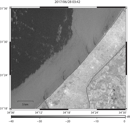
To prepare the oil spill dataset for the training procedures, all the oil spills inside the pre-processed images were labelled as oil objects jointly by two authors who are experienced human interpreters. The oil objects were defined by bounding boxes, which show the extent of oil spills, with the open-source image annotation tool LabelImg (Tzutalin Citation2015). Note that look-alikes were not labelled but regarded as background information. Manual inspection of oil spills is based on experience and prior information including location, wind and weather condition, the period of the year and differences in their shapes compared to surroundings (Solberg et al. Citation1999; Topouzelis Citation2008). In the Eastern Mediterranean Sea, algal bloom is a common reason for look-alikes due to nutrient sources of coastal origins (e.g. increasing use of fertilizers) and strong current systems (Barale, Michel Jaquet and Ndiaye Citation2008). shows an example of preprocessed data including look-alikes due to different reasons along with some visible land sourced oil spills. Algae blooms appear as dark formations with spiral patterns, which are driven by surface currents (e.g. north of the image). Dark formations surrounded by algal blooms might be low wind areas. The blue rectangle marks a region with regular oil spills from land sources. Red bounding boxes show locations of oil spills, and dark formations near coastal areas are possibly induced by wind and waves. Look-alikes make it more difficult to tell if there are oil spills in the scene and to annotate them correctly. Oil spills can be distinguished from look-alikes due to their different patterns, and also from experience of collecting regular oil spills from the area (see for examples).
Figure 4. An example of look-alikes shown in Sentinel-1 SAR data along with some visible land sourced oil spills. The blue rectangular area has regular land sourced oil spills, which are annotated with red bounding boxes. Apart from oil spills, there are dark formations due to algae blooms (spiral patterns), low wind areas (near algae blooms) and possible wind and wave effects (in coastal area near oil spills).
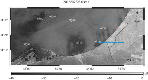
Figure 5. An example showing clear oil spills coming from land sources. This figure has the same extent as the blue outlined area shown in .
shows a heat map based on the amount of oil spills collected and annotated in this study; there are in total 9768 labelled oil objects from 2015 to 2018. Regions with frequent oil spills might be related to shipping routes, locations of oil fields and oil terminals, and some regular pollution from land sources. The figure shows relatively frequent oil spills at the northern access of the Suez Canal, which has high density of ship traffic especially due to tankers transiting between Suez Canal and ports in the Eastern Mediterranean or Western Europe (O’Hagan Citation2007). It shall be noted that the amount of oil spills was calculated from the labelled oil objects, which are not exact polygons showing the oil spill location but the extent of the spill defined by its bounding box.
2.3. Dataset
The pre-processed images cover areas with dimensions of around px and
px for the ascending and descending tracks, respectively. However, most of the labelled oil objects only occupy areas of less than
px, which makes it difficult for the object detector to target objects. In addition, the object detector requires a certain model input size, which might change the aspect ratios of images. To avoid training the object detector on distorted images, the pre-processed images were cropped into smaller sizes to fit the model input size. The images were cropped based on the positions of the labelled oil objects. Each oil object has one corresponding cropped image; however, it might happen that there are several oil objects in one cropped image generating several cropped images with similar coverage. To avoid the same oil objects appearing in multiple images, this study filtered out most of the duplicated ones manually. Checking the labels in the dataset and filtering out the duplicated oil objects required around 40 h of work for each year (e.g. from 1 January 2017 to 31 December 2017). As the cropped images were designed based on labelled oil objects, each cropped image includes at least one oil object. Note that this does not mean that every image must contain an object during the detection process. The object detector learns not only the given objects but also the regions without annotations as background during training. Therefore, it is expected to return no object if there is none to detect. The cropped images have dimensions of
px, where
is equal to the maximum of the model input size and the edge lengths of the object bounding box. The model input size in this study is
px. Large oil objects could therefore result in images with sizes greater than the model input size, so they will be resampled when put into the model. With this approach, however, long and slim oil objects in such images might become undetectable when they are resampled. shows examples of long and slim oil spills, which possibly resulted from ships. The images cover areas of around 1220 km2 and 770 km2, respectively. These kinds of oil spills are usually discharged from moving ships. In the beginning, there is a larger amount of oil released, and as the ship keeps moving the amount decreases resulting in the oil trace becoming gradually slimmer. The slimmer part of oil spills might be barely visible to the object detector. Hence, these kinds of images were manually examined again, and images with long and slim oil objects were tiled into several sub-images in order to avoid the oil spills becoming undetectable. On the contrary, if the oil objects inside the image were long and wide, they were not altered to let the model learn the entire shape of the oil spill.
Figure 6. Examples of long and slim oil spills. The areas of the images are around 1220 km2 and 770 km2, respectively.
The cropped images (including the tiled images after examination) were then put into different size groups based on the sizes of the largest oil objects inside. Oil spills in bounding boxes with an area smaller than 12,500 px (i.e. 5 km2) were categorized as small oil objects, and those with bounding boxes greater than or equal to 100,000 px (i.e. 40 km2) were categorized as large oil objects. The rest of the oil spills with areas in-between were regarded as medium objects. However, certain small objects were regarded as undetectable tiny objects and had their annotations removed. In this study, tiny objects were defined as follows:
where ,
and
respectively refer to the heights of the object, image and model input;
refers to the corresponding width.
is the pixel threshold for defining tiny objects. The first scenario in subsection 3.1 aims to find a suitable value for
.
shows the amount of oil objects per size category in the dataset after removing the tiny objects with px. An imbalance with regard to the amount of objects per category can be observed because there are comparatively fewer larger oil spills than smaller ones. In addition, the larger oil spills seems to have higher shape complexity, which might be more difficult to detect. To alleviate the imbalance of oil spills in different sizes and enhance the ability of detecting larger oil spills, data augmentation was applied, focusing on images with larger oil objects. The idea of data augmentation is to increase the amount of data by applying slight modifications to the original dataset. The second scenario in subsection 3.1 provides a comparison of model performance when applying rotation data augmentation on specific groups before model training.
Table 1. Amount and percentage of oil objects with different sizes in the dataset from 2015 to 2018 after removing tiny objects.
After data augmentation, the whole dataset was split into training, validation and test sets. Different-sized oil objects were balanced between the sets and the objects were put into the different sets with a relative proportion of . Considering that there are seasonal algae in the study area, it was ensured that training, validation and test sets all contained images from different seasons and images in different sets should not originate from the same SAR acquisitions.
2.4. Yolov4 object detection algorithm
Deep learning-based object detection algorithms work in three essential stages: feature extraction, object localization and classification. Feature extraction, the so-called backbone of an object detector, finds the representation of the input images as feature maps by using a backbone network. The network has different layers to learn multiple levels of features, and is usually trained on a large labelled dataset (e.g. ImageNet (Deng et al. Citation2009)). The object localization stage finds the area of the image that potentially contains an object, which is also known as the region of interest (ROI). Then, the classification stage fine tunes the proposed region and outputs the final prediction with the class of the objects. The object localization stage and the classification stage are usually called the head. An additional stage for collecting feature maps might also be included between the backbone and the head, which is regarded as the neck.
Two-stage object detection algorithms refer to those using two different networks to achieve object localization and classification in two different steps, which means that the classifier needs to detect the object class in each ROI. This step makes the object detection comparatively slow and uses a high amount of computational resources. However, one-stage object detection algorithms combine object localization and classification into one step with only a single deep neural network. YOLO is an example of a one-stage object detection algorithm (Redmon et al. Citation2016). One-stage object detectors are usually regarded as more efficient but less accurate. However, the accuracy and speed of the recent one-stage object detector YOLOv4 has been improved by implementing a new architecture, introducing Bag-of-Freebies (BoF) and Bag-of-Specials (BoS), and including mosaic, a new data augmentation method (Bochkovskiy, Wang and Mark Liao Citation2020; Wang, Bochkovskiy and Mark Liao Citation2021). In the preliminary stage, this study compared the model performance of the trained objectors with and without applying mosaic data augmentation; the AP of the trained detectors on test set is 55.54% and 30.34%, respectively. The results highlight the improvement of the model from applying mosaic.
shows the overall structure of YOLOv4. YOLOv4 uses CSPDarknet53 as its backbone, which applies Cross Stage Partial Network (CSPNet) (Wang et al. Citation2020) to update the previous YOLOv3 backbone Darknet53. It further reduced the need of computational resources as CSPNet proposes a richer gradient combination while reducing the requirement of computational resources to solve the vanishing gradient problem during the training stage (Wang et al. Citation2020). CSPDarknet53 extracts feature maps through five residual blocks (Bochkovskiy, Wang and Mark Liao Citation2020), followed by Spatial Pyramid Pooling (SPP) and a modified Path Aggregation Network (PANet) as the neck. SPP enhances the receptive field, which represents all the pixels from feature maps with an impact on results. PANet has the ability to keep spatial information in order to improve the object localization. In the last stage, three yolo layers are applied as the head. Feature maps of different scales are collected in order to find objects with different sizes. The model input size in this study is px, and detection feature maps down-sampled by factors of 8, 16 and 32 are generated. Therefore, the detection feature maps have dimensions of
,
and
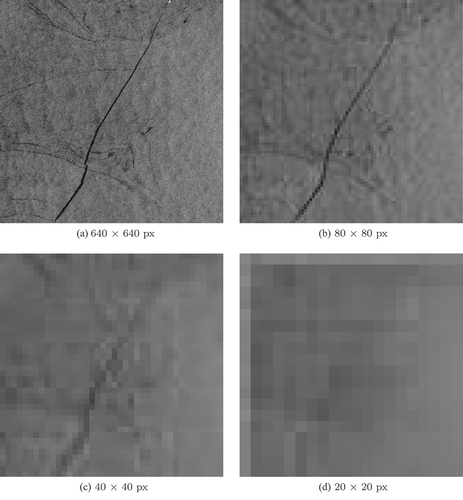
px. In order to picture how much information can be obtained in different scales, shows the down-sampled images. The idea is that large objects can be detected with smaller scale (e.g.
px) and small objects need larger scale (e.g.
px) to include the necessary details.
Figure 7. Overall structure of YOLOv4. The backbone CSPDarknet53 extracts feature maps through 5 residual blocks. SPP and PANet are applied to enhance the respective field and improve the object localization, respectively. Feature maps of different scales are extracted by three yolo layers in the last stage in order to detect objects with different sizes. The figure incorporates elements modified from (Li et al. Citation2020; Hu and Wen Citation2021).
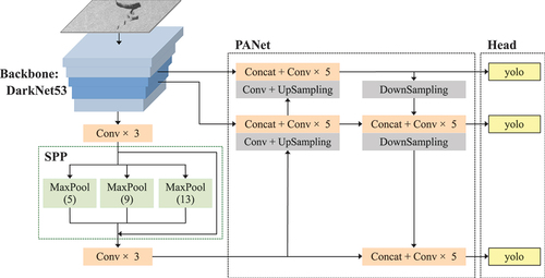
Figure 8. Images with oil spills in different scales. The images were downsampled to different dimensions. Note that the original image has a size of px, which is greater than the model input size; thus, the image was downsampled to
px as shown in (a) (see Subsection 2.3 for detailed explanation).
3. Results
This section presents the results obtained from training the deep learning model for oil spill detection. Different scenarios are considered and shown in the following subsections. Subsection 3.1 determines the parameter in EquationEquation (1)
(1)
(1) to find a suitable measure to remove tiny oil objects. Subsection 3.2 then investigates if adding additional rotation data augmentation can help improve the model performance. For training the model an Nvidia GeForce RTX 3080 GPU with 10 GB VRAM was used, which took around 7.5 h for each training run with 6000 iterations. As an initial estimation, it would require at least around
image patches with a size of
px and overlap of 40 px to cover the whole study area. Detecting oil spills in these images by the trained model would take around 1 min.
To evaluate the performance of an object detector, its predictions are compared to ground truth data. As there is no real-world ground truth oil spill data available, ground truth data refers to the manually inspected objects described in subsection 2.2 in this study. The comparison between predictions and ground truth can be summarized by a confusion matrix with four components: True Positive (TP), False Positive (FP), False Negative (FN) and True Negative (TN). TP shows oil objects that are correctly detected by the object detector. FP refers to cases where oil objects are detected but they do not match the ground truth. On the contrary, undetected oil objects are regarded as FN. TN is generally not applied in object detection as background is not defined in ground truth and also not present in detections.
shows different detections of the same oil spill. The red bounding box denotes the manually inspected oil object and the yellow bounding boxes mark the detections. is the best match because it shows the largest overlap with the ground truth data. However, a concrete definition of correct detection should be defined. Intersect over union (IoU) is therefore used as it indicates how close the predicted area of an object is to the ground truth bounding box. It is defined as follows (Everingham et al. Citation2010):
Figure 9. Examples showing detections with different IoU.
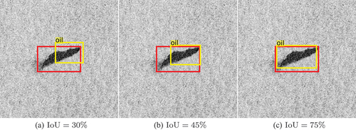
where and
respectively refer to the intersection and union of the bounding boxes of the prediction (
) and the ground truth (
). The IoU threshold is usually applied to define whether a detection is TP or FP. In this study, the IoU threshold is defined as 50%, which means that only detections with
and have the same class prediction (i.e. oil) are TP.
Based on TP, FP and FN, the recall and precision measures are used and given as follows (Goutte and Gaussier Citation2005):
Recall represents the sensitivity to detect objects, that is, among all the ground truth data, the amount of objects that are correctly detected. Precision describes the number of correctly detected objects in comparison to the ground truth data. It is desirable that the object detector has both high precision and recall. Based on these two measures, AP is defined as an average of precision values from a set of recall for a single class as follows:
where is recall,
is the precision at discrete recall values
. In this study, AP is calculated as an average of precision values from 11 equally spaced recall values as discrete approximation of EquationEquation (4)
(4)
(4) analogous to the VOC2007 challenge (Everingham et al. Citation2010).
The trained models are evaluated by a comparison of their AP on the test sets with an IoU threshold of 50%, which was calculated with the help of a tool developed in Cartucho, Ventura and Veloso (Citation2018) and modified by the authors. Based on results emerging from different scenarios, an improved trained model along with a selection of detection results on different types of oil spills are described in subsection 3.3. This study also compares the performance of the models trained by YOLOv4 and the well-known two-stage object detection algorithm Faster RCNN.
3.1. Remove annotations of tiny objects
In the preliminary stage of the study, the trained model generated spurious detections where no oil spill was visible. One possible explanation is that during the training procedure of the object detector, the input image is down-sampled by factors of 8, 16 and 32 in the object detection stage. Small objects need a larger scale (i.e. smaller downsampling factor) to capture their features, and objects below a certain size might be undetectable. There are tiny oil spills regularly released in the Eastern Mediterranean Sea, and hence it is possible that some of the labelled objects are invisible for the model but their annotations are in the training dataset. As a result, the trained model lacks the capability of detecting the extents of objects correctly and generates some random detections with oil spills improperly framed or even exceeding the image boundary (see .
Figure 10. Examples for removal of tiny objects with varying from a previous study. The yellow bounding boxes denote the detections with the confidence scores, and the red bounding boxes mark the ground truth oil spills (Yang, Singha and Mayerle Citation2021).
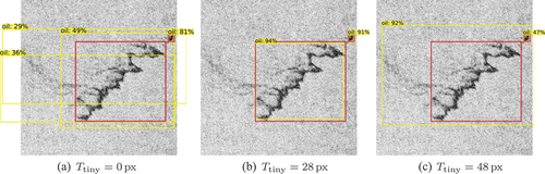
As an initial test for removing the annotations of objects satisfying EquationEquation (1)(1)
(1) with
equal to
,
and 48 px, shows examples of detections from different trained models (Yang, Singha and Mayerle Citation2021). In the model regards the oil object to cover an area larger than the oil spill of interest. It seems that the model was ‘guessing’ the extent of the oil object as it could not find the margin of the object well. Generally, applying a pixel threshold seems to help prevent excess detections when comparing with . Comparing
equal to
and 48 px, the trained object detector in more clearly defines the extents of oil spills than the one in . Based on this result, the removal of the annotation for tiny objects with smaller thresholds was examined further. shows the amount of objects used in different cases and the model performance achieved. The four test cases are all, rm_tiny_14, rm_tiny_20 and rm_tiny_28 where
equals
,
,
and 28 px, respectively. When no object annotation is removed (all), the AP on the test set was 61.64%. After removing tiny objects, the AP was slightly improved. However, with
px the model performance actually decreased to 55.54% AP on the test set. A possible reason is that there were some removed objects observable in the image but without any annotation, so the model was misled. Overall, the test case rm_tiny_20 with
px showed the best performance.
Table 2. Amount of objects in the training, validation and test sets for different cases that were used in scenario 1 (subsection 3.1), along with the AP of the trained models on the respective validation and test sets.
This scenario outlines the limitation of the object detector when targeting tiny objects. Small oil spills are not always clearly distinguishable from their surroundings due to the resolution of satellite imagery, making it difficult to properly define their extents. However, this limitation is in line with the capability of human observers who may disregard the detected tiny oil spills because of the described uncertainty. Nevertheless, the imbalance among oil spills of different sizes (see ) might lead to a lower capability of detecting larger oil spills although they lead to more serious environmental damage. Therefore, decreasing the false-negative rate on detecting larger oil spills seems to be more important than increasing the ability of tiny object detection. The following subsection compares the model performance on oil spills of different sizes and provides scenarios to improve the oil spill detector.
3.2. Additional data augmentation
shows the absolute and relative amount of oil objects used after the annotations of the tiny objects have been removed with px. As there are small oil spills regularly appearing in the study area, 72.3% of all oil objects in the dataset have a bounding box area smaller than 12,500 px (i.e. 5 km2). In order to let the model detect oil spills of different sizes, additional rotation data augmentation was applied to images with larger oil objects in this scenario. All images were first categorized into large, medium and small image groups in relation to the size of the largest oil object inside. Images in the groups large and medium were rotated by 90° along with their annotations; the augmented image sets are noted as L90_aug and M90_aug, respectively. shows the model performance for three different cases and the amount of oil objects per size group. The case orig is the same as case rm_tiny_20 in subsection 3.1. The cases L90 and L90_M90 include the images from the case orig along with the additional augmented images from L90_aug and both L90_aug and M90_aug, respectively. Note that these different cases were tested on the same test set for model performance assessment. In these cases, there were in total 576 images in the test set.
Table 3. Amount of objects in the small, medium and large size groups for different cases that were used in scenario 2 (subsection 3.1), along with the AP of the trained models on the respective validation and test sets.
Among the three cases, the case L90 shows the best model performance with an AP of 69.53% and 70.55% on the validation and test sets, respectively. On the other hand, the AP of the trained object detector in the case L90_M90 on the validation and test sets is 69.99% and 65.05%, respectively, which shows that the model is not well generalized and indicates possible model over-fitting to random patterns in the validation set. To further examine the models for their behaviours when detecting oil spills of different sizes, the test set was then split into three different subsets according to oil spill sizes (following the definition in ). There were 387, 141 and 48 images in small, medium and large test subsets, respectively. shows AP in the different cases and on the three subsets. The results in L90 are better on small and medium oil spills but worse on large oil spills in comparison to the case orig, which does not fulfil the aim of improving the model performance on larger oil spills. In the case L90_M90, which not only considered the large subset but also included the medium subset for data augmentation, the model was trained on a higher complexity of oil spills. The model performance has improved for detecting large oil spills; however, it appears to be worse on small and medium subsets. Supporting this observation, shows different sizes of oil spills detected in the three different cases with the confidence scores as well as the manual inspections outlined in red.
Figure 11. Examples of oil spills in (a) large and (b) medium subsets detected in different cases described in subsection 3.1. The red bounding boxes denote the manually inspected oil spills; the detection results are shown with different colors along with confidence scores. As detection results from the cases orig and L90 show high consistency with the manual inspection in (b), the detections are not shown in the image to avoid confusion.
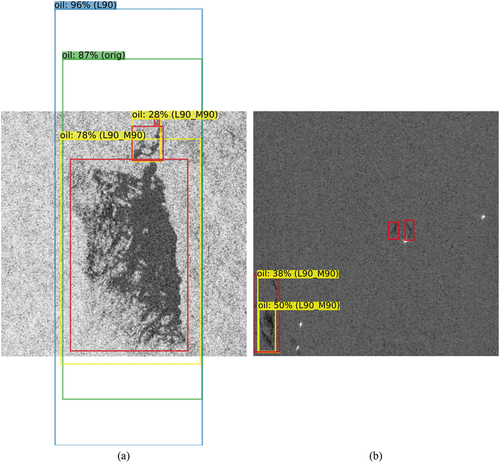
Table 4. The AP of the trained models on the test sets with oil spills of different sizes in scenario 2 (subsection 3.1).
shows a large oil spill, which is manually labelled as three oil objects as they were not connected with each other. The oil spill was detected by the models from the cases orig and L90 as one object; however, the extents were not well predicted. One possible reason could be that images covering large areas with slim and long oil spills were tiled into several sub-images for training (see Subsection 2.3). With this approach, the model did not properly learn the entire shape of these oil spills and how they were separated from their surroundings. The IoU of the largest labelled oil object and detections from these two cases is 47.46% and 34.95%, respectively. On the other hand, the case L90_M90 has IoU of 71.70% and 71.61% for the upper and bottom detections, respectively. As the case L90_M90 included more medium oil spills, the ability of detecting margins seems to be improved. shows examples of small and medium oil spills. As predictions in cases orig and L90 are similar to the manually labelled oil objects, only the case L90_M90 is shown. Regarding the oil spill on the left-hand side, all the models detect it as two oil spills; one small bounding box covers the bottom part of oil spill and the other large one covers the whole oil spill. The IoU of the three detections covering the whole oil spill from cases orig, L90 and L90_M90 is 64.67%, 76.67% and 81.57%, respectively. Regarding the two oil spills in the middle, the model from case orig has respective IoU of 75.06% and 81.03% for the two oil spills (from left to right); the model from case L90 has IoU of 74.60% and 79.77%, respectively. However, in the case L90_M90 they were not detected.
In summary, by applying additional rotation augmentation on images with large and medium oil objects (i.e. case L90_M90), the detection of large oil spills has improved. It is likely that including data augmentation on differently shaped oil spills could help the performance of the object detector. However, in the dataset most of the large oil spills appear along with small oil spills, which means that the rotation data augmentation was also applied on some small oil objects. It is possible that the model was over-fitting on oil objects with similar shapes, especially for small oil spills, which usually appear as round shapes as shown in . As there are drawbacks for either the case L90 or the case L90_M90, it was decided to not apply the additional data augmentation before further examination. A possible approach would be to apply additional data augmentation on oil spills with high complexity and to use fewer small round objects from the dataset and balancing different-sized oil objects, but the total amount of objects used for training should also be considered.
Figure 12. Examples of small round oil spills in the study area. The shown images cover areas of around 164 km2 each.
3.3. Oil spill detection with YOLOv4
According to subsection 3.1, objects regarded as tiny objects following EquationEquation (1)(1)
(1) with
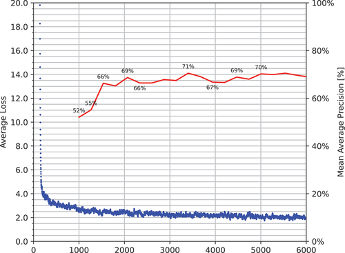
px were removed. Though additional rotation augmentation was proven to be beneficial for large oil spill detection, it might cause over-fitting on small and medium oil spills based on the results in subsection 3.2; as a result, this technique was not applied in the following. YOLOv4 offers several built-in data augmentation techniques, which, unlike the rotation data augmentation discussed in the previous subsection, are applied to all input images. Overall, colour space data augmentation (e.g. saturation, exposure and hue values) seems to be beneficial in this study. shows the average loss calculated during the training in blue and the mean average precision (mAP) on the validation set in red after 1000 iterations. The average loss indicates the differences between the ground truth values and predicted values from the model. In general, the training stops after the average loss no longer decreases. Note that mAP is the mean of the AP on different classes. As only one class was in use, mAP is equal to AP in this study. The AP on the validation and test sets is 69.10% and 68.69%, respectively. The model performance is similar on the validation and test sets, which indicates that the object detector is not dependent on the given training or validation datasets.
Figure 13. Average loss calculated during the training (blue), and AP on validation set (red) after 1000 iterations.
As mentioned in subsection 2.4, one-stage object detection algorithms are usually considered to have high efficiency but low accuracy compared to two-stage methods. To evaluate the performance of the YOLOv4-based model, this study uses a two-stage object detection algorithm, Faster RCNN, as a baseline assessment. Faster RCNN with feature pyramid networks (FPN) as backbone was trained with the help of the Detectron2 framework, which is implemented in PyTorch (Wu et al. Citation2019). shows training information along with the AP on the validation and test sets of the two object detection algorithms. The iterative training was stopped when the average loss converged. As Faster RCNN requires more training iterations, it took almost double the time of YOLOv4. The Faster RCNN-based model has its AP on the training and validation sets of 70.33% and 70.26%, respectively. Comparing the two trained models, the performance seems to be similar; however, the faster training time of YOLOv4 is advantageous for development stage where training has to be performed several times.
Table 5. Training information along with the AP of the trained models on the validation and test sets from YOLOv4 and Faster RCNN, the two well-known object detection algorithms.
In the following, various examples of oil spills detected by the YOLOv4-based model will be shown in . Manually inspected oil spills are denoted as red bounding boxes and the detection results are outlined in yellow along with confidence scores. Note that some oil spills are separately annotated as they are not actually connected, but may appear like a continuous oil spill in the figures due to scaling.
Figure 14. Examples of long oil spills detected by the trained object detector described in subsection 3.3 . Some long and wide oil spills were well detected in (a) and (b); however, some slim oil spills were not confidently detected in (c) and (d).
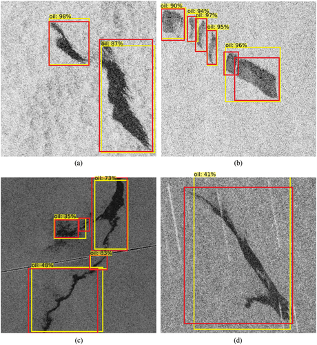
Figure 15. Examples of areas covering numerous small oil spills, which were mostly well detected. Note that some oil spills were detected by the trained object detector (in yellow) but not marked as manually inspected oil spills (in red). These oil spills satisfy the definition of tiny object in EquationEquation (1)(1)
(1) with
px and their annotations were removed.
![Figure 15. Examples of areas covering numerous small oil spills, which were mostly well detected. Note that some oil spills were detected by the trained object detector (in yellow) but not marked as manually inspected oil spills (in red). These oil spills satisfy the definition of tiny object in EquationEquation (1)(1) ifhobj<himg⋅Ttiny/hmodel[px]∪wobj<wimg⋅Ttiny/wmodel[px]\break⇒Obj∈Objtiny(1) with Ttiny=20 px and their annotations were removed.](/cms/asset/708e1c67-f4a1-47c8-8e9e-1526918706d1/tres_a_2109445_f0015_c.jpg)
Figure 16. Examples of oil spills which appeared near look-alikes. Oil spills were well detected in (a), but it was not clearly if it detected oil spills or look-alikes in (b).
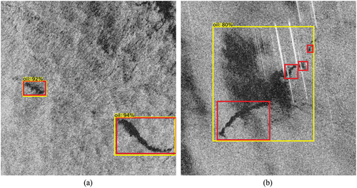
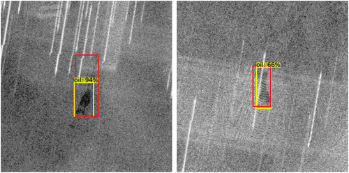
Figure 17. Examples of oil spills with interference caused by active transponders, which influence certain regions constantly. However, the object detector was still able to detect these oil spills well.
shows examples of relatively long oil spills, which are generally detected. are examples of wide and long oil spills, which were detected similarly to the given annotations. Considering slim and long oil spills, show that they were not as confidently detected as the wider ones and their margins were not well detected. These kinds of oil spills usually cover a large area and form complicated shapes due to ocean currents (see also ). As previously explained (see subsection 2.3), slim and long oil spills were tiled into several sub-images in case the oil spills might otherwise be too thin for the model to learn and to detect. Therefore, the full shape of these kinds of oil spills was not well learned, especially as large oil spills only occupied 5.5% of the collected oil objects (see ), so there were even less long and slim oil spills. As a result, especially long and slim oil spills were not as well detected as wider ones.
As mentioned in section 1, small oil spills regularly occurred in the study area, so detecting oil spills of this kind is also an aim of this study. shows examples of those oil spills, which were small but numerous. Note that there were some oil spills detected by the object detector but not annotated as they were regarded as tiny objects defined by EquationEquation (1)(1)
(1) with
px and removed from the annotations. It seems that the object detector possesses a good capability of detecting these small oil spills and it could actually detect tiny objects below the given
. Based on the comparisons between different
shown in subsection 3.1, applying
px resulted in the best AP. Objects are defined as tiny when either dimension is smaller than the given
in EquationEquation (1)
(1)
(1) . However, the aspect ratio of the object was not considered so that the model might be able to detect objects even if one dimension is smaller than
. Examining the behaviour of the model for detecting small oil objects more closely might help, such as providing some man-made oil objects with different sizes and aspect ratios and designing a more rigorous rule for tiny object definition.
shows examples of oil spills near look-alikes. In , oil spills were detected well even with look-alikes nearby. However, it is not clear in if the object detector detected the oil spill correctly as it was covered by look-alikes. Note that in order to not mislead the model, oil spills covered by look-alikes were not annotated (as shown in the figure). As look-alikes were included in the dataset only when they appeared near oil spills, the trained detector might recognize only limited types of look-alikes. Increasing the amount of look-alikes used as background information during training might help improve the ability of distinguishing oil spills and look-alikes.
In the Eastern Mediterranean Sea, active transponders are commonly used for security reasons and interfere with the SAR signal, in some regions constantly. When the active transponders happen to be operating in similar frequency domain as SAR signal, it might lead to constructive or destructive interference. shows oil spills covered by these interfering signals. However, the object detector could still detect the main parts of the oil spills. Regular oil spills in certain areas are likely caused by the same or similar sources, which result in less complexity in types and shapes of oil spills. Hence, the object detector was able to learn and detect them well.
4. Discussion and conclusion
To tackle the need of an early warning system for detecting oil spills on a regular basis in the Eastern Mediterranean Sea, this study evaluated the possibility of using a YOLOv4-based object detection algorithm for automatic detection of oil spills. In this study, a total of 5930 Sentinel-1 scenes from 2015 to 2018 were used, which contain 9768 oil spills. After carrying out a variety of scenarios to find suitable parameters and data augmentation methods in subsections 3.1 and 3.2, the trained object detector was presented in subsection 3.3 . The AP of the object detector, with IoU threshold equal to 50%, on the validation and test sets is 69.10% and 68.69%, respectively. Comparing it to the Faster RCNN-based model, which has AP of 70.33% and 70.26% on the validation and test sets, respectively, the two models have similar performance. However, training the Faster RCNN model took almost twice as long. In recent years, more studies have focused on machine learning and deep learning techniques using large amounts of SAR data. Some well-performing deep learning-based oil spill detection methods are discussed in the following. Note that different studies used different measures to evaluate the model performance, and the definitions of these measures may even be slightly different.
One previous study used a total of 1112 SAR images and trained with different semantic segmentation methods. IoU for different classes is used as performance metric in the study, and U-Net and DeepLabv3+ achieve IoU of 53.79% and 53.38% on the class oil spill, respectively (Krestenitis et al. Citation2019). Another study presented an improved DeepLabv3+ and used a total of 35 Sentinel-1 scenes; it obtains IoU of 91.58% for the class oil spill (Ma et al. Citation2022). One other study used 14 ALOS PALSAR and 7 Sentinel-1 scenes and trained the CBD-Net, where it reached 84.20% and 91.20% precision on datasets from the two different satellite missions, respectively (Zhu et al. Citation2022). As a small amount of images leads to a lack of complexity in types, shapes and backscatter values of oil spills in SAR images, the models trained with fewer images performed better than the ones with larger datasets. However, two previous studies applied Mask-RCNN on similar amounts of data (i.e. 2000–3000 images) and achieved 98.7% precision on oil spill detection and 65% mean IoU for different classes in (Yekeen and Balogun Citation2020) and (Emna et al. Citation2020), respectively. The various sources of oil spills, purposes of those studies and even the difficulties of obtaining ground truth oil spills make it difficult to compare the results from these different studies.
With reference to the previously mentioned studies, the trained oil spill detector has reasonably good performance, especially for detecting oil spills with different sizes and even when oil spills were covered by the interference of active transponders. However, long and slim oil spills as well as their extent were not confidently detected. As shown in subsection 3.2, it is hard to train a model which performs well with a wide variety of object sizes. Increasing the amount of long and slim oil spills and balancing different size oil spills used for training might help improve the model performance in future.
Oil spills near look-alikes were also distinguished well, but oil spills covered by look-alikes were not always clearly detected. It appeared that the model was misled as in these cases, it detected the whole look-alike and the oil spill covered by it as one big oil spill. In this study, all images used for training contained at least one oil object. This means the patterns of look-alikes were only learned when there were oil spills nearby, so that adding images with only look-alikes (i.e. without any annotation) into training as background information might help the object detector to differentiate better between oil spills and look-alikes caused by various sources.
The collected oil spills were mostly related to shipping routes, oil terminals and transboundary shipping ports, and depending on the circulation systems in different regions oil spills may drift differently. It is possible that the detector may have inferior performance in other areas, where the majority of oil spills originate from different sources (e.g. oil platforms and natural seepage). To detect oil spills in other regions, it is possible to apply transfer learning, which uses the knowledge of the existing model in new tasks. Instead of learning from scratch, the existing model will be regarded as a pre-trained model and further trained on additional datasets with oil spills of different origins. Likewise, the capability of the current detector on different SAR sensors cannot be guaranteed, but applying transfer learning for different SAR sensors is feasible and should be straightforward for C-band sensors (e.g. RADARSAT Constellation Mission). Nevertheless, the provided trained object detector is a suitable module to set up an oil spill surveillance system in the Eastern Mediterranean Sea. The results of this study are the basis of an improved oil spill detector, which lays the ground for building an efficient early warning system in the near future.
Acknowledgements
This study is part of the DARTIS project, which was supported by the German Federal Ministry of Education and Research under Grant number 03F0823B. The authors wish to thank Copernicus for providing Sentinel-1 data on Open Access Hub. We would also like to thank ESA for developing SNAP and the user support provided on the Scientific Toolbox Exploitation Platform (STEP) forum. We are grateful to the developers and all the contributors of YOLOv4 for their wonderful work at https://github.com/AlexeyAB/darknet.
Disclosure statement
No potential conflict of interest was reported by the author(s).
Additional information
Funding
References
- Abdulla, A. and O. Linden. 2008. Maritime Traffic Effects on Biodiversity in the Mediterranean Sea: Review of Impacts, Priority Areas and Mitigation Measures. Malaga, Spain: IUCN Centre for Mediterranean Cooperation .
- Al-Ruzouq, R., M. Barakat a Gibril, A. Shanableh, A. Kais, O. Hamed, S. Al-Mansoori, and M. Ali Khalil. 2020. “Sensors, Features, and Machine Learning for Oil Spill Detection and Monitoring: A Review.” Remote Sensing 12 (20): 3338. doi:10.3390/rs12203338.
- Barale, V., J. Michel Jaquet, and M. Ndiaye. 2008. “Algal Blooming Patterns and Anomalies in the Mediterranean Sea as Derived from the SeaWifs Data Set (1998-2003).” Remote Sensing of Environment 112 (8): 3300–3313. doi:10.1016/j.rse.2007.10.014.
- Bochkovskiy, A., C.-Y. Wang, and H.-Y. Mark Liao. 2020. “YOLOv4: Optimal Speed and Accuracy of Object Detection.” arXiv preprint arXiv:2004.10934.
- Brekke, C. and A. H. Solberg. 2008. “Classifiers and Confidence Estimation for Oil Spill Detection in ENVISAT ASAR Images.” IEEE Geoscience and Remote Sensing Letters 5 (1): 65–69. doi:10.1109/LGRS.2007.907174.
- Cartucho, J., R. Ventura, and M. Veloso. 2018. “Robust Object Recognition Through Symbiotic Deep Learning in Mobile Robots.” In 2018 IEEE/RSJ International Conference on Intelligent Robots and Systems (IROS), Madrid, Spain, 2336–2341.
- Chang, Y.-L., A. Anagaw, L. Chang, Y. Chun Wang, C.-Y. Hsiao, and W.-H. Lee. 2019. “Ship Detection Based on YOLOv2 for SAR Imagery.” Remote Sensing 11 (7): 786. doi:10.3390/rs11070786.
- Deng, J., W. Dong, R. Socher, L. Li-Jia, K. Li, and L. Fei-Fei. 2009. “ImageNet: A Large-Scale Hierarchical Image Database.” In 2009 IEEE Conference on Computer Vision and Pattern Recognition, Miami, FL, USA, 248–255. IEEE.
- Devadharshini, S., R. Kalaipriya, R. Rajmohan, M. Pavithra, and T. Ananthkumar. 2020. “Performance Investigation of Hybrid YOLO-VGG16 Based Ship Detection Framework Using SAR Images.” In 2020 International Conference on System, Computation, Automation and Networking (ICSCAN), Pondicherry, India, 1–6.
- Emna, A., B. Alexandre, P. Bolon, M. Véronique, C. Bruno, and O. Georges. 2020. “Offshore Oil Slicks Detection from SAR Images Through the Mask-RCNN Deep Learning Model.” In 2020 International Joint Conference on Neural Networks (IJCNN), Glasgow, UK, 1–8. IEEE.
- European Maritime Safety Agency. 2017. “The CleanSeaNet Service: Taking Measurements to Detect and Deter Marine Pollution.” Brochure. http://www.emsa.europa.eu/csn-menu/download/2913/2123/23.html
- European Space Agency. 2020 “SNAP - ESA Sentinel Application Platform V8.0.” http://step.esa.int
- Everingham, M., L. Van Gool, C. K. Williams, J. Winn, and A. Zisserman. 2010. “The PASCAL Visual Object Classes (VOC) Challenge.” International Journal of Computer Vision 88 (2): 303–338. doi:10.1007/s11263-009-0275-4.
- Fiscella, B., A. Giancaspro, F. Nirchio, P. Pavese, and P. Trivero. 2000. “Oil Spill Detection Using Marine SAR Images.” International Journal of Remote Sensing 21 (18): 3561–3566. doi:10.1080/014311600750037589.
- Ghorbani, Z. and A. H. Behzadan. 2021. “Monitoring Offshore Oil Pollution Using Multi-Class Convolutional Neural Networks.” Environmental Pollution 289: 117884. doi:10.1016/j.envpol.2021.117884.
- Goutte, C. and E. Gaussier. 2005. ”A Probabilistic Interpretation of Precision, Recall and F-Score, with Implication for Evaluation.” In Advances in Information Retrieval, edited by D. E. Losada and J. M. Fernández-Luna, Vol. 3408, 345–359. 04. Berlin Heidelberg: Springer.
- Hovland, H. A., J. A. Johannessen, and G. Digranes. 1994. “Slick Detection in SAR Images.” In 1994 IEEE International Geoscience and Remote Sensing Symposium (IGARSS), Pasadena, CA, USA, Vol. 4, 2038–2040.
- Hu, G. and C. Wen. 2021. “Traffic Sign Detection and Recognition Based on Improved YOLOv4 Algorithm.” International Journal of Computer Applications Technology and Research 10 (6): 161–165. doi:10.7753/IJCATR1006.1006.
- Krestenitis, M., G. Orfanidis, K. Ioannidis, K. Avgerinakis, S. Vrochidis, and I. Kompatsiaris. 2019. “Oil Spill Identification from Satellite Images Using Deep Neural Networks.” Remote Sensing 11 (15): 1762. doi:10.3390/rs11151762.
- Li, Y., H. Wang, L. M. Dang, T. N. Nguyen, D. Han, A. Lee, I. Jang, and H. Moon. 2020. “A Deep Learning-Based Hybrid Framework for Object Detection and Recognition in Autonomous Driving.” IEEE Access 8: 194228–194239. doi:10.1109/ACCESS.2020.3033289.
- Ma, X., J. Xu, P. Wu, and P. Kong. 2022. “Oil Spill Detection Based on Deep Convolutional Neural Networks Using Polarimetric Scattering Information from Sentinel-1 SAR Images.” IEEE Transactions on Geoscience and Remote Sensing 60: 1–13.
- Nieto-Hidalgo, M., A. Javier Gallego, P. Gil, and A. Pertusa. 2018. “Two-Stage Convolutional Neural Network for Ship and Spill Detection Using SLAR Images.” IEEE Transactions on Geoscience and Remote Sensing 56 (9): 5217–5230. doi:10.1109/TGRS.2018.2812619.
- O’Hagan, C. 2007. “Use of GIS for Assessing the Changing Risk of Oil Spills from Tankers.” In Conference paper presented at 3rd Annual Arctic Shipping Conference, St Petersburg, Russia , 17–20.
- Pavlakis, P., D. Tarchi, and A. J. Sieber. 2001. On the monitoring of illicit vessel discharges using spaceborne SAR remote sensing - a reconnaissance study in the Mediterranean sea. In Annales des Télécommunications, Vol. 56 (11), 700–718. doi:10.1007/bf02995563.
- Polinov, S., R. Bookman, and N. Levin. 2021. “Spatial and Temporal Assessment of Oil Spills in the Mediterranean Sea.” Marine Pollution Bulletin 167: 112338. doi:10.1016/j.marpolbul.2021.112338.
- Redmon, J., S. Divvala, R. Girshick, and A. Farhadi. 2016. “You Only Look Once: Unified, Real-Time Object Detection.” In 2016 IEEE Conference on Computer Vision and Pattern Recognition (CVPR), Las Vegas, NV, USA, 779–788.
- REMPEC. 2002. Towards Sustainable Development of the Mediterranean Region: Protecting the Mediterranean Against Maritime Accidents and Illegal Discharges from Ships. Malta. http://hdl.handle.net/20.500.11822/11254.
- Ronci, F., C. Avolio, M. Di Donna, M. Zavagli, V. Piccialli, and M. Costantini. 2020. “Oil Spill Detection from SAR Images by Deep Learning.” In 2020 IEEE International Geoscience and Remote Sensing Symposium (IGARSS), Waikoloa, HI, USA, 2225–2228. IEEE.
- Saadoun, I. M. 2015. Impact of Oil Spills on Marine Life Larramendy, Marcelo L., Soloneski, Sonia. Emerging Pollutants in the Environment-Current and Further Implications. Rijeka, Croatia: IntechOpen. p. 75–105. doi:10.5772/60455.
- Shaban, M., R. Salim, H. Abu Khalifeh, A. Khelifi, A. Shalaby, S. El-Mashad, A. Mahmoud, M. Ghazal, and A. El-Baz. 2021. “A Deep-Learning Framework for the Detection of Oil Spills from SAR Data.” Sensors 21 (7): 7 doi:10.3390/s21072351. .
- Singha, S., T. J. Bellerby, and O. Trieschmann. 2013. “Satellite Oil Spill Detection Using Artificial Neural Networks.” IEEE Journal of Selected Topics in Applied Earth Observations and Remote Sensing 6 (6): 2355–2363. doi:10.1109/JSTARS.2013.2251864.
- Singha, S., R. Ressel, D. Velotto, and S. Lehner. 2016. “A Combination of Traditional and Polarimetric Features for Oil Spill Detection Using TerraSAR-X.” IEEE Journal of Selected Topics in Applied Earth Observations and Remote Sensing 9 (11): 4979–4990. doi:10.1109/JSTARS.2016.2559946.
- Solberg, A. H. S. 2012. “Remote Sensing of Ocean Oil-Spill Pollution.” Proceedings of the IEEE 100 (10): 2931–2945. doi:10.1109/JPROC.2012.2196250.
- Solberg, A. H. S. and R. Solberg. 1996. “A Large-Scale Evaluation of Features for Automatic Detection of Oil Spills in ERS SAR Images.” In 1996 IEEE International Geoscience and Remote Sensing Symposium (IGARSS) Lincoln, NE, USA, Vol. 3, 1484–1486.
- Solberg, A. H. S., G. Storvik, R. Solberg, and E. Volden. 1999. “Automatic Detection of Oil Spills in ERS SAR Images.” IEEE Transactions on Geoscience and Remote Sensing 37 (4): 1916–1924. doi:10.1109/36.774704.
- Stevens, J. 2020. “NASA Earth Observatory Map.” Accessed 8 September 2020. https://visibleearth.nasa.gov/images/147190/explorer-base-map
- Surkes, S. 2021. “Satellite Images of Oil Slicks off Coast Show Recent Spill Far from a One-Off.” The Times of Israel, February 28 https://www.timesofisrael.com/satellite-images-of-oil-slicks-off-coast-show-recent-spill-far-from-a-one-off/
- Topouzelis, K. N. 2008. “Oil Spill Detection by SAR Images: Dark Formation Detection, Feature Extraction and Classification Algorithms.” Sensors 8 (10): 6642–6659. doi:10.3390/s8106642.
- Topouzelis, K. and A. Psyllos. 2012. “Oil Spill Feature Selection and Classification Using Decision Tree Forest on SAR Image Data.” ISPRS Journal of Photogrammetry and Remote Sensing 68: 135–143. doi:10.1016/j.isprsjprs.2012.01.005.
- Tzutalin. 2015. “LabelImg.” https://github.com/tzutalin/labelImg
- Wang, C.-Y., A. Bochkovskiy, and H.-Y. Mark Liao. 2021. “Scaled-YOLOv4: Scaling Cross Stage Partial Network.” In Proceedings of the IEEE/CVF Conference on Computer Vision and Pattern Recognition (CVPR) Nashville, TN, USA, June, 13029–13038.
- Wang, C.-Y., H.-Y. Mark Liao, W. Yueh-Hua, P.-Y. Chen, J.-W. Hsieh, and I.-H. Yeh. 2020. “CSPnet: A New Backbone That Can Enhance Learning Capability of CNN.” In Proceedings of the IEEE/CVF Conference on Computer Vision and Pattern Recognition Workshops Seattle, WA, USA, 390–391.
- Woodhouse, I. H. 2006. Introduction to Microwave Remote Sensing. Boca Raton, FL, USA: CRC press.
- Wu, Y., A. Kirillov, F. Massa, L. Wan-Yen, and R. Girshick. 2019. “Detectron2.” https://github.com/facebookresearch/detectron2
- Yang, Y.-J., S. Singha, and R. Mayerle. 2021. “Fully Automated SAR Based Oil Spill Detection Using YOLOv4.” In 2021 IEEE International Geoscience and Remote Sensing Symposium (IGARSS) Brussels, Belgium, 5303–5306.
- Yekeen, S.T. and A.L. Balogun. 2020. “Automated Marine Oil Spill Detection Using Deep Learning Instance Segmentation Model.” The International Archives of Photogrammetry, Remote Sensing and Spatial Information Sciences 43: 1271–1276. doi:10.5194/isprs-archives-XLIII-B3-2020-1271-2020.
- Zhu, Q., Y. Zhang, Z. Li, X. Yan, Q. Guan, Y. Zhong, L. Zhang, and D. Li. 2022. “Oil Spill Contextual and Boundary-Supervised Detection Network Based on Marine SAR Images.” IEEE Transactions on Geoscience and Remote Sensing 60: 1–10.