High resolution C-band SAR backscatter response to peatland water table depth and soil moisture: a laboratory experiment

ABSTRACT

Carbon storage and active carbon sequestration within peatlands strongly depend on water table depth and soil moisture availability. With increasing efforts to protect and restore peatland ecosystems, the assessment of their hydrological condition is highly necessary but remains challenging. Synthetic aperture radar (SAR) satellite observations likely offer an efficient way to obtain regular information with complete spatial coverage over northern peatlands. Studies have indicated that both radar backscatter amplitude and phase are sensitive to peatland condition. Very recently, Differential Interferometric Synthetic Aperture Radar (DInSAR) has been reported as being capable of monitoring ground deformation patterns at the millimetre scale, which are a response to peatland hydrological condition. To further investigate the promise of SAR for peatland monitoring, a laboratory-based polarimetric C-band SAR system was used to acquire the dynamic radar behaviour of a 4 m (l) ×1 m (w) × 0.25 m (d) reconstructed peatland. A forced 4-month drought was introduced with very-high-resolution imagery taken every 2 hours, capturing details of the vertical backscatter patterning through the peat at the centimetric scale. The results showed a clear coherent response both in radar backscatter amplitude and phase to change in water table level and soil moisture. Similar responses were seen across all polarizations. Phase demonstrated a coherent and deterministic change across the experiment; the average differential phase increase across all polarizations was 118° for 17 cm of water table drawdown. Interpreted as the physical movement of the surface, this corresponded to 8.3 mm of surface subsidence. Both phase and amplitude changes were near-linear with changes in the water table depth; amplitude showed a correspondingly strong concomitant mean decrease of 7 dB across all polarizations during the experiment. The results demonstrate the close sensitivity of radar backscatter to hydrological patterns in a peatland ecosystem. The phase result, in particular, strongly supports the notion that differential phase from satellites can be utilized to measure ground deformation as a proxy for the hydrological state.

1. Introduction

Peatlands are a type of wetland ecosystem, with unique acidic and waterlogged conditions where plant material does not fully decay, accumulates, and ultimately forms a deep peat layer with high carbon density (Moore 1989). Storage and sequestration of carbon by healthy, wet peatlands play an important role in regulating the global carbon (C) emissions (Bonn et al. 2016), especially as peatlands remain the largest terrestrial carbon store (Gorham 1991). Besides being crucial for helping to address climate change, peatlands are important for preserving global biodiversity, providing drinking water, and reducing flood risks (Emilie et al. 2013). Despite the high value of these ecosystems, human activity (drainage, extraction, conversion to agricultural land and afforestation) globally has led to a shift of peatlands functioning as a C source rather than sink (Leifeld and Menichetti 2018). Peatlands are now annually contributing about 5% of the total anthropogenic CO₂ equivalent emissions (Gewin 2020) with the highest degradation and associated emissions coming from Southeast Asian and European peatlands (Urák et al. 2017). Global and national level conservation efforts to protect and restore peatlands have increased in the past years; however, a further increase of GHG emissions is predicted, due to peatland degradation reaching up to 8% of the global anthropogenic carbon dioxide emissions by the year 2050 (Urák et al. 2017; Swindles et al. 2019).

More than ever, the assessment of peatland ecosystem condition in pristine, damaged, or restored peatlands is necessary, but remains challenging, especially over larger areas in remote locations. While traditional monitoring methods by carrying out field measurements can give precise information about the health status of the peatland, they can be expensive, time-consuming, covering small areas and time periods, and often in locations that are not easily reachable (Lees et al. 2018). The use of satellite imagery for monitoring purposes has increased tremendously in the past years, as new satellite data with higher spatial and temporal resolutions have become publicly available (Connolly et al. 2011; Artz et al. 2019). Optical sensors can provide wide spectral information and can be very useful for peatland vegetation (Xue and Su 2017) and hydrological condition (Angela and Bryant 2009) monitoring. The main disadvantage of optical sensors remains the dependency on cloud-free conditions and although various gap-filling techniques to account for missing data exist (Poggio, Gimona, and Brown 2012), cloud cover over Northern peatlands is widely present, making it challenging to achieve a regular resampling interval. Imagery from radar instruments, on the other hand, can be harder to interpret but provide more regular data that are independent of persistent cloud or smoke cover (Kasischke, Melack, and Craig Dobson 1997).

Monitoring peatland hydrological condition is important because water table depth and soil moisture are the predominant factors driving biogeochemical processes in peatlands and can have the overriding control on greenhouse gas emissions (Hilbert, Roulet, and Moore 2000; Evans et al. 2021). Excessive lowering of water level (WL) in peatlands can lead to peat subsidence, oxidation, and large amounts of carbon being released to the atmosphere (Nusantara, Hazriani, and Suryadi 2018; Yehui, Jiang, and Middleton 2020). High water level and high soil moisture are also necessary environmental conditions for the regeneration of characteristic peatland vegetation in restoration projects (Alderson et al. 2019), as well as reducing peatland vulnerability to wildfires (Meingast et al. 2014). As drought periods in northern latitudes are predicted to increase both in frequency and severity under climate change (Fenner and Freeman 2011; Swindles et al. 2019), a reliable monitoring system for peatland hydrological condition is necessary.

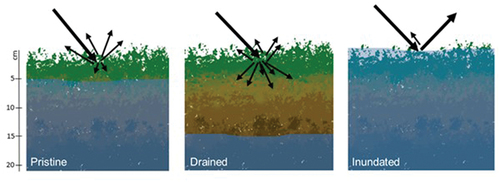
Radar backscatter is a measure of the energy fraction returned from a target compared to the energy of the incident field. Besides the radar instrument properties (frequency, polarization, incidence angle), the intensity of the backscatter will vary depending on the physical properties of the scene (Bernard et al. 1982; Widhalm, Bartsch, and Heim 2015). The ability of a scene feature to reflect the radar signal is dependent on the target’s physical properties: surface roughness and geometry of the target, and dielectric properties, which are a proxy for water content (Ulaby, Batlivala, and Dobson 1978; Irena, Pottier, and Cloude 2003). Therefore, the largest influence on backscattering in unforested peatland areas is soil moisture and surface roughness, vegetation obscuring the soil, soil texture, and, to a minor degree, soil surface temperature, and peat bulk density (Beale et al. 2019). Pristine peatlands, normally having very high water content and therefore high dielectric constant, will reflect more signal and so have a higher backscatter compared to targets with low dielectric constant, e.g. drained peat soils (Figure 1). Parts of near-natural peatlands can also be completely inundated, resulting in a specular-like surface where radar signal would be reflected away from the sensor resulting in very low backscatter values.

Figure 1. Radar backscattering characteristics based on the water level position in peatlands.

SAR sensitivity to water table depth and soil moisture change in peatlands has been reported previously using satellite data over near-natural, drained, and managed sites, re-wetted and restored peatlands (Kasischke et al. 2009; Torbick et al. 2012; Dabrowska-Zielinska et al. 2016; Kim et al. 2017; Bechtold et al. 2018; Asmuß, Bechtold, and Tiemeyer 2019; Bechtold et al. 2020; Lees et al. 2021). Furthermore, radar has been shown to have the potential to monitor soil moisture along with vegetation regeneration to assess if peatland restoration efforts are successful and determine if additional interference is necessary (White et al. 2020).

The incoherent component (amplitude or power) of the radar signal has a strong sensitivity to dielectric constant; therefore, radar backscatter intensity has been used in various studies to examine radar signal sensitivity to soil moisture and water table depth in peatlands (Wagner et al. 2007). The coherent (phase) component difference of the radar signal between two or more satellite radar acquisitions has been used to infer surface movement and vegetation height changes using the Interferometric Synthetic Aperture Radar (InSAR) technique (Bamler and Hartl 1998). Many factors impact both the backscattering intensity and the phase, therefore accounting for a single parameter such as soil moisture can be challenging. What makes it even more complex is the diverse nature of peatland landscapes, and even though a reliable monitoring system to follow peatland hydrological condition is highly desirable, a universal retrieval of peatland soil moisture from SAR data is hard to develop and site-specific or peatland type-specific studies are more common (Meingast et al. 2014). This has encouraged efforts to fully understand and exploit SAR capabilities for peatland condition monitoring, including peatland water level and soil moisture monitoring. Recent efforts have highlighted InSAR, specifically, the APSIS (Advanced Pixel System using Intermittent Small Baseline Subset (SBAS)) method, formerly known as ISBAS (Bradley et al. 2022) as a potential satellite-based peatland condition monitoring system due to its ability to capture annual, seasonal, and interseasonal movement of the peat (Alshammari et al. 2018, 2020; Tampuu et al. 2020). This method has been developed to focus on non-urban land areas where usage of conventional Differential InSAR (DInSAR) techniques is challenging due to the temporal decorrelation (Sowter et al. 2013) and has shown potential for peatland condition characterization (Cigna et al. 2014; Alshammari et al. 2018, 2020). These InSAR methods have shown the ability to follow the shorter-term seasonal peat surface movement, often referred to as ‘bog breathing’ (Morton and Heinemeyer 2019) or ‘bog surface oscillation’ (Howie and Hebda 2018), which corresponds to dynamics of water and gasses within the peat, typically showing drawdown during the warmer months and recharge and uplift during the winter months (Alshammari et al. 2019).

Most studies utilizing radar instruments for peatland hydrological condition monitoring have used satellite data. This study made use of laboratory SAR measurements of a peatland sample. The arrangement in the laboratory permitted us to isolate the backscattering dependency on changes in peatland hydrological status, allowing us to eliminate or control perturbing factors, such as micro-topography, vegetation, and weather. Additionally, it removed any atmospherically induced distortions associated with satellite image processing, particularly regarding the differential phase (Cigna et al. 2014; Cheng et al. 2012). Previous studies have reported various relationships, from very high correlations between SAR and peatland hydrological status to no obvious correspondence between the parameters, so here we have tested to what extent the radar backscatter – water table drawdown relationship could be explained if no other major factors were to influence the backscattering. The main aim of this study was to assess the SAR signal sensitivity to drought in peatlands based on an analysis of 6 months long TP radar series. Specific objectives were as follows: a) explore TP SAR for peatland hydrological condition monitoring, including usage of different polarizations, b) investigate the radar backscatter dependency on different peatland hydrological regimes, c) analyse how the weighted mean backscatter height within a peatland changes with drought conditions. The findings from this study enhance the understanding of how radar backscatter interacts with peat and blanket bog vegetation, add useful knowledge to both radar backscatter and InSAR for peatland research literature, and help with improving methods for continuous observation of peatland condition, which are needed to enable appropriate peatland management and conservation decisions being taken (Lees et al. 2018; Alshammari et al. 2019).

2. Materials and methods

2.1. Laboratory measurement

Longer-term peat surface movement can indicate peat accumulation (in case of a build-up of partially decomposed organic matter) or subsidence (due to drainage, compression, and decay of organic matter) (Alshammari et al. 2018). Although promising, these studies have highlighted the difficulty of validating the accuracy of obtained results as it often requires a comparison of large-scale satellite data to small-scale field observations and underlines the need for further research to improve quantitative validation of the InSAR vertical velocity (Alshammari et al. 2018). Most studies utilizing radar instruments for peatland hydrological condition monitoring have used current and previous radar imaging satellite mission data, a few have used airborne radar data (Baghdadi et al. 2001), but to the best of our knowledge, this is the first time high-resolution radar measurements have been collected in a controlled laboratory-environment setup.

2.1.1. ‘Bog in the box’ experimental setup

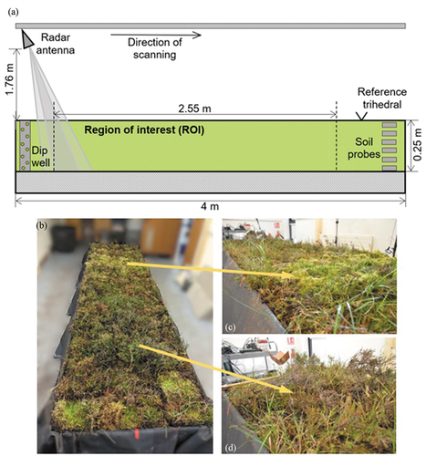
Blocks of vegetation-covered peat were collected from an upland blanket bog in the Eastern Cairngorms, Scotland (56.9 N, −3.15 E; ca 650 m). The thirty-two 30 (length) × 50 (width) × 25 (depth) cm samples were transported in plastic boxes to the University of Reading by courier. Here, they were removed from their containers and reconstructed into a 400 (l) × 100 (w) × 25 (d) cm blanket bog section within the trough of the Reading Radar Facility (Figure 2) for microwave measurement. The laboratory was equipped with four full spectrum 80 W LED grow lights to facilitate the continued growth of the blanket bog vegetation.

Figure 2. a) Schematic of the radar measurement system and experiment setup. The bog was surrounded on its bottom and sides by a waterproof butyl rubber liner and sat upon a stable bed of dry sand (25 cm deep). b) Photograph of the ‘Bog in the box’ laboratory setup. c) Sphagnum segment, representing predominantly moss vegetation. d) Ericaceous (heather) segment, representing moss layer covered with dwarf-shrub vegetation.

Once in the trough, the reconstructed peatland was inundated with deionized water up to a water table depth of 5 cm below the trough edge. Afterwards, the peat was watered regularly with artificial rainwater using a manual hand-held water sprayer simulating local rainfall. We followed Noble et al. (2017) and used a synthetic rainwater concentrate (at a pH of around 5.5). The simulation of rainfall occurred 2–3 times a week, with 2–3 l of water added per time, keeping the water table at a steady level. Blanket bogs are ombrotrophic ecosystems, where water and nutrients are gained mainly by rainfall, mist, or snow, resulting in an acidic environment low in nutrients. Regular rainfall simulations were carried out for 2 months prior to the beginning of the experimental drought period. The drought period was simulated as a total drought with no rainfall simulations first until WL reached the bottom of the trough (22 cm below the edge of the trough) and continued until the deepest soil moisture probe reported a drop to 0.8 volumetric water content (VWC). The experiment simulated a 117-day long drought period, after which the bog was re-wetted back to the original WL state of 5 cm below the surface by adding 280 l of deionized water over a 10-day period (7 rainfall simulations, 40 l per time).

The bog vegetation assemblage represented a typical Eastern Cairngorms M18-type blanket bog (Elkington et al. 2001), dominated by Calluna vulgaris as the primary ericaceous species, Eriophorum spp. and other sedges, and Sphagnum capillifolium as dominant Sphagnum species; however, other Sphagnum and other moss species were present in lower proportions. To assess if different vegetation had an impact on the backscattering signal, three 25 cm segments with predominantly Sphagnum moss layer only (Figure 2c) and three 25 cm segments with heather and sedge/grass species above the moss canopy (Figure 2d) were identified.

A dip well (perforated PVC well pipe) and six soil volumetric water content (VWC) and temperature sensors (5TM, METRE) were installed across the trough at depths of 3, 5, 7, 10, 18, and 22 cm. VWC and soil temperature (°C) data from the probes, along with a sensor for room air temperature (°C), were connected to a Campbell CR1000 data logger and logged every 30 min. Daily water table depth measurements at ± 1 were gathered manually using the dip well.

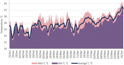
The average room temperature throughout the experiment was 17.7°C, with lower temperatures experienced during the night, and higher during the day and towards the end of the experiment (Figure 3). These conditions are similar to the July and August climate averages (1981–2010 period) for the Braemar climate station in the vicinity of Ballater (MET Office 2021).

Figure 3. Average, minimum, and maximum air temperatures in the laboratory during the experiment.

The experimental setup allowed us to eliminate or closely control factors that can influence the interpretation of the radar backscattering signal in peatlands, allowing us to closely investigate the backscattering dependency on peatland hydrological regimes. First, possible changes in surface roughness and vegetation structure due to wind, grazing, or burning were eliminated. Second, we were in control of the hydrological regime of the experimental setup. By introducing acclimatization (normal amount of precipitation), drought (no precipitation), and re-wetting phases, we were able to directly inspect the radar signal response to changes in soil moisture and water level regimes. The experimental setup also prevented lateral water losses. As the experimental duration was relatively short (6 months during which environmental conditions were kept largely the same), vegetation growth effects are likely to have been negligible. There were no open water bodies, which are common in peatland environments; therefore, a specular reflection of the radar signal, which can greatly impact backscattering values, has not been assessed in this experiment.

We acknowledge that a laboratory experimental setting will almost unavoidably diverge from the real-world environment, but this way we can achieve a well-controlled repeatable environment where the findings are descriptive of the environment at large.

2.1.2. Radar data collection

The radar measurements were carried out using the indoor component of the Reading Radar Facility at the University of Reading. A roof-mounted linear scanner is centrally located above and down the length of the plywood measurement trough. A cluster of four C-band antennas was centrally mounted on the scanner 1.8 m above the trough, pointing forward at 10° from nadir, being sufficiently close to each other to use a monostatic approximation. Their 3 dB across-track beamwidth maps onto the width of the trough. By switching in the appropriate transmit-receive antenna pair, the four scans sequentially captured the VV, VH, HH, HV polarimetric responses. Data collection was accomplished by sequentially stepping the antennas monotonically along the scanner in 1.5 cm intervals over a 375 cm aperture. At each position, microwave data were collected at 1601 equally spaced points across a frequency range of 4–8 GHz. Scans were collected in sets of four, where each scan provided capture at a single polarization, and took 20 minutes to complete a set. Data sets were collected at 6-hour intervals prior to the drought and at 2-hour intervals during the drought and rewetting phases. (Morrison and Wagner 2020) provide more details of the microwave RF sub-system. The system response was calibrated using precision radar cross-section (RCS) targets with the method of Kamal, Ulaby, and Ali Tassoudji (1990) just prior to the start of the experiment. System changes thereafter were monitored and corrected for using a reference trihedral and sphere. Measurement precision in signal power and phase is estimated to be 0.2 dB and 5° degrees, respectively.

Out of the 6012 scans, 356 were collected prior to the drought, 5060 during the drought and 596 during the rewetting experiment. In the analysis, we considered the backscattering values both in co-polarizations: VV, HH, and cross-polarization (mean of HV and VH).

While the full length of the trough was 4 m, a region of interest (ROI) of 255 cm was used in the radar imagery analysis to avoid edge effects at both ends of the trough and exclude the regions where the calibration target and soil moisture equipment were located (Figure 2).

2.1.2.1. Tomographic profiling and weighted mean height

Tomographic profiling (TP) is a SAR-like imaging technique designed specifically for gathering vertical backscattering profile data through biogeophysical volumes (Morrison and Bennett 2014). Unlike in SAR imaging, the antennas are aligned along-track and so only collect data for a transect directly below the scanner. Post-measurement, the antenna beam is synthetically sharpened by coherent summation across a sub-aperture of sample points. The aperture is moved on one point along the aperture and the process repeated, and so on. In this way, a series of overlapping vertical ‘sounding profiles’ are obtained, highlighting the radar backscatter pattern through the target of interest. By adding phase ramps across the sample points, the beam was configured to look forward at an incidence angle of 10°. TP imagery is not true tomographic imagery (Morrison and Bennett 2014) as it lacks any angular discrimination in the across-track (across the trough) direction. The target returns in this direction are considered collapsed down to a central slice down the centre of the trough. Previously, the TP method has been successfully used in laboratory and field studies to investigate the internal structure of snowpacks (Morrison et al. 2008), forest canopies (Morrison, Bennett, and Solberg 2013), dry soils (Morrison and Wagner 2020), and subsurface archaeology (Morrison 2013).

In the analysis, the differential phase is interpreted as a bulk movement of the peat sample. The change in the vertical displacement of the peat, $D$, can be written as:

(1) $D=\frac{\lambda \mathrm{\Phi }}{\mathrm{c}\mathrm{o}\mathrm{s}i\hspace{0.17em}\times \hspace{0.17em}360\times 2}\hspace{0.17em},$(1)

where λ is the wavelength (5 cm in this study), i is the incidence angle (here, 10°), and Φ is the measured phase difference.

The TP scheme enables the possibility to analyse the vertical backscattering signal; we applied weighted mean height (WMH) to investigate the effective position of the vertical backscattering signal and its change over the duration of the drought. The WMH is calculated as:

(2) $\bar{x}=\frac{{\sum }_{i=1}^n{w}_i{x}_i}{{\sum }_{i=1}^n{w}_i}\hspace{0.17em},$(2)

in which $\bar{x}$ is the weighted mean height, $x$ is the height of the specific pixel, and $w$ its corresponding amplitude value (Yrttimaa et al. 2020). WMH shows at what height the backscatter is the strongest, and the time series of radar measurements can be used to investigate whether this height changes over time.

2.2. Statistical modelling

Using the R programming environment (R Core Team 2021), an empirical relation between SAR backscatter and the measured water level was assessed. A linear regression model was fitted to the water level and radar backscatter data (both backscatter strength and differential phase), and significance levels for each polarization were noted as highly significant (p < 0.001). The soil probe data and backscattering response were analysed using the R ‘mgcv’ package (R Core Team 2021), and a generalized additive model (GAM) model was fitted between probes at all depths and the backscattering response. The significance levels between each of the polarizations and probes at different depths were then assessed and the GAM model was then refitted using data from the statistically significant probes only (p-values <0.05). The model was then tested for autocorrelation using Partial Autocorrelation Function (PACF), indicating significant correlations only at the first lag, followed by correlations that are not significant. The response backscattering values and values computed from the model matched up well indicating a good fit with no obvious outliers or deficiencies in the model found.

3. Results

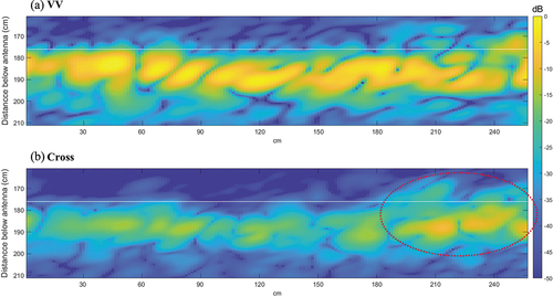
In this section, both the cross- and co-polarized radar backscatter signal strength and differential phase time-series trends throughout the whole duration of the experiment are presented. Figure 4 shows example TP images obtained across the ROI in co-polarization (VV) and cross-polarization just prior to the drought period, reconstructed for an incidence angle, i, of 10°. The backscatter from the ROI surface obtained in co-polarizations (VV, HH) is notably stronger in relation to cross-polarization returns. It is understood that, in the presence of vegetation, a signal that has been transmitted in V (H) can bounce once or multiple times from randomly oriented plant structures, producing a cross-polarization return (here in H (V)) (Srivastava et al. 2009). The increase in the cross-polarized signal strength present after 200 cm in Figure 4 is associated with greater vegetation depths from the presence of dwarf shrubs.

Figure 4. Cross-sectional views of the backscattering values from the selected peatland ROI (255 cm (l) × 100 cm (w) × 50 cm (d)) before the drought, constructed using a 10° incidence angle. The position of the trough is shown by the horizontal white line. The red dotted oval indicates an area with heather cover and hence increased volume scattering in cross-polarization (calculated as mean of HV and VH) can be seen.

The time series of the radar measurements showed a clear decrease in backscattering strength (Figure 5a) and concomitant phase increase (Figure 5b) over the progression of the drought. The change of backscattering strength and phase varied between polarizations but showed the same characteristic patterns. After 117 days of no precipitation, a 6.0 dB decrease and about 140° phase increase equal to 10 mm subsidence were observed, when using VV polarization and 10° incidence angle; 7.1 dB and 8 mm in HH polarization; 7.3 dB and 8 mm in cross-polarization. Once the rewetting took place, the backscattering increased in all polarizations, but only by 1 dB on average, not reaching the pre-drought values. Similarly, phase values decreased up to 24 degrees after rewetting, but the pre-drought level was not met, potentially indicating semi-permanent peat subsidence (peat compaction) due to the drought.

Figure 5. Time series of radar backscattering (a) and phase (b) measurements reconstructed using VV, HH, and cross-polarization and 10° incidence angle. Each backscatter datum is the result of an incoherent summation of pixels across the selected ROI (255 cm (l) × 1 m (w) × 50 cm (d)), extracted for each image in the time series. The red dashed lines indicate the beginning (21/01/2021) and end (17/05/2021) of the simulated drought period.

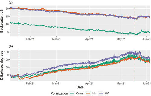
We observed that the co-polarization values on average were 10.0 dB stronger than cross-polarized signatures. The two co-polarizations had very similar values throughout the experiment, with HH backscattering values being on average 0.4 dB stronger. VV, HH values varied between 19.7 and 20.7 dB before the drought and 13.7 to 13.6 dB after 117 days of drought. Cross-polarization values were 11.0 dB prior to the drought and 3.7 dB by the end. The mean backscatter value between all polarizations was 17.1 dB prior to the drought and 10.3 dB by the end of it.

3.1. Radar backscattering signal strength and phase response to change in water table depth

The radar backscatter was strongest at the beginning of the experiment when the WL was closest to the surface (5 cm): about 20.5 dB in co-polarized data and 11.1 dB in cross-polarization. After 95 days of drought, when WL had just reached the bottom of the trough, the backscattering had lowered by 4.8 dB (VV), 5.5 dB (HH), 5.9 dB (cross).

All polarizations demonstrated a phase increase, with VV polarizations having the highest phase increase during the drought. After 95 days of drought, when WL had reached the bottom of the trough, the differential phase had increased by 120° or 8.5 mm (VV), 86° or 6.1 mm (HH), 84° or 5.9 mm (cross).

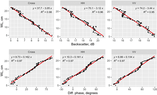
After fitting a linear regression model to water level and radar backscatter data, a strong negative correlation with R² >0.94 was found between backscattering values and the water level in all polarizations (Figure 6). Similarly, the radar differential phase had a strong positive correlation (R² >0.96) with the observed water level in all polarizations.

Figure 6. Correlation analysis between water level and radar backscatter (Figure 5a) and differential phase (Figure 5b) during the drought period (95 days with WL reaching 22 cm below the surface).

3.2. Radar backscattering signal strength response to change in soil moisture

The radar signal relationship with soil moisture varied between the depth of the probe placement (Figure 7). The probes closest to the surface show a clear drying curve with a decrease in volumetric water content of the soil and a decrease in the backscattering values as the drought progressed. The probe placed at 22 cm depth remained largely saturated (80% VWC) even after 117 days of drought and had no significant relationship with the backscattering values in any polarization mode. The second deepest probe (18 cm) had a notable correlation with the backscattering only once WVC dropped below 80%, which was 90 days after the beginning of the drought.

Figure 7. Soil moisture and backscattering strength response to drought (117 days of drought). Drying curves of the 6 soil moisture probes at 3–22 cm depth.

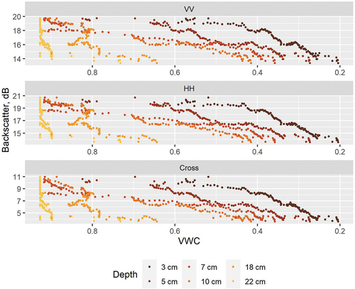
The fitted GAM model showed a significant relationship (p-values <0.05) between the radar backscatter and probes at almost all depths, but the strongest relationships were observed with probes at 3–10 cm depth. When the GAM model was refitted using these probes only, the model showed a resulting R² of 0.98, indicating an excellent fit with residuals being equally and randomly spaced (Figure S1 and S2 in the Supplementary material). The corresponding backscattering values and values computed from the model matched up very well indicating a good fit with no obvious outliers or deficiencies in the model found, clearly showing the strong linkage between volumetric water content in the peat and the radar backscattering response.

3.3. Weighted mean height

Using the advantage of vertical resolution from the TP scheme, an analysis of how the effective weighted mean height (WMH) of the vertical backscattering signal changed over the duration of the drought was carried out. Figure 8 shows how during the first month of drought the weighted mean height of backscatter from the ROI did not report a significant lowering in any of the polarizations, even though the WL had lowered by 6 cm. The following 45 days showed a slow decrease in the WMH by −0.46/-0.85/-0.61 cm in VV/HH/cross-polarization, respectively; at this point, WL had dropped by 13.5 cm. Finally, the remaining period of the drought (last 45 days and 500 scans) showed a further decrease leading to a difference of −1.35/-1.7/-2.18 cm in VV/HH/cross-polarization compared to the initial values at the beginning of the drought. The WL reached the bottom of the trough halfway through this interval, but the WMH values continued to decrease; therefore, it can be noted that the WMH is not only influenced by the water level in the peatland but also the continued peat compaction and soil moisture decrease.

Figure 8. ROI backscatter weighted mean height change throughout the 117-day drought period.

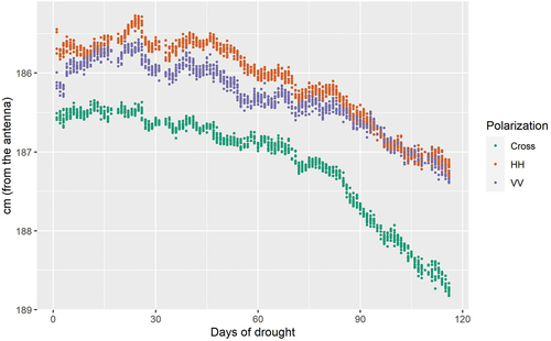
Compared to the differential phase results, it can be noted that both measures indicate a distance increase during the drought period between the peat and the radar instrument, but while the differential phase showed a 0.8–1 cm subsidence between the three polarizations, the WMH values lowered by 1.4–2.2 cm. The highest subsidence values were observed in VV polarization using the differential phase, while cross-polarization backscatter had the biggest drawdown looking at the WMH.

4. Discussion

This study assessed the sensitivity of C-band TP radar signal backscatter and phase and peatland hydrological parameters (soil moisture and water table depth) over different hydrological regimes. This laboratory-based experiment included collecting unique high-resolution SAR data signatures from a 4 × 1 m reconstructed peatland for a period of 6 months, including a simulated drought. It is the first study to utilize the TP SAR system over peatland and demonstration of the vertical profile of the radar backscattering signal through peat and typical blanket bog vegetation and its relationship with soil hydrological status.

The time-series analysis in this study demonstrated a close sensitivity of backscattering strength and radar phase to hydrological patterns in a peatland ecosystem with R² >0.9 when other factors influencing radar backscattering were controlled for. The strong correlation between radar signal and moisture status observed in this study suggests that it is likely the main controller of backscattering values in sparsely vegetated peatlands when looking at short-term periods. This observation is in agreement with results from Asmuß, Bechtold, and Tiemeyer (2019), who found WTD to be the major factor controlling backscattering strength when looking at drained temperate grasslands with underlying peat soils. Other studies with good correlation results between backscatter strength and peatland soil moisture note that C-band backscatter can be a good indicator of moisture status, but the best results can be achieved only in non-forested sites (Kasischke et al. 2009; Dabrowska-Zielinska et al. 2016; Millard and Richardson 2018).

During the drought period of the experiment, the radar phase had a steady upward trend interpreted as arising from the increasing distance between the radar and peat surface, relating to water level decline and surface subsidence. Small oscillations were observed in the first part of the experiment, often concurrent with changes in room temperature, which could be explained by the peat settling in, water movement and distribution through the peat mass and to a lesser extent the entrapped gas dynamics in peatlands (Strack, Kellner, and Waddington 2006). Previous studies focussing on the phase component of the radar signal have investigated the peatland surface oscillations over different time periods. Methods using repeated InSAR measurements have been able to track both long-term peat subsidence or uplift and shorter-term surface movement, mainly connected with the dynamics of water and gasses (Alshammari et al. 2019, 2018, 2020; Bradley et al. 2022) used APSIS to investigate seasonal amplitude of peat swelling as well as multiannual surface motion. They concluded that the condition of the peatland determines these ecohydrological measures as there exist certain patterns, such as subsidence over the years, amplitude of the peat swelling and the surface motion peak timings between near-natural peatlands in good condition and degraded sites. These studies had highlighted the uncertainty in the validation of the InSAR interpretation due to the massive scale difference between large-scale satellite data and small-scale field observations. Our study used a much higher accuracy SAR instrument, reducing this gap and confirmed that the phase component can maintain coherence and be highly sensitive to the water drawdown and peat subsidence. A study by Kim et al. (2017) used field-collected WTD and radar satellite-derived soil moisture estimates over the Great Dismal Swamp (R² = 0.76 with Radarsat-1 C-band and R² = 0.67 with ALOS PALSAR L-band) and similarly to our findings noted that both the radar backscatter intensity and the InSAR time series can correspond well with water table depth drawdown. Our WMH analysis has shown how the vertical SAR backscatter through the peat corresponds well with the water level drawdown and peat subsidence and has a close similarity to the differential phase change through the drought period.

Besides the dynamics of the water level, vegetation is normally the other factor having the biggest influence on radar backscatter and cause of InSAR decorrelation (Lee et al. 2020). The excellent model fit between radar backscatter and both water level and soil moisture achieved in this laboratory study points out how the hydrological condition monitoring over peatlands could be improved significantly if other elements influencing the radar backscatter would be accounted for. Indeed, recent studies have highlighted the importance of correcting dynamic vegetation effects when estimating soil moisture and WL in peatlands (Bechtold et al. 2018; Lees et al. 2021). In this study, we observed dwarf shrub and grasses-dominated segments having a different backscattering behaviour to Sphagnum-covered segments (Figure S3 in the Supplementary material). While both Sphagnum moss and heather-dominated transects resulted in reduced backscattering values over time during the drought, a distinction between the two groups was observed. At optimal conditions, Sphagnum moss can have water content as much as 20 times heavier than its dry weight (Pang et al. 2020). Due to the retention of water, the higher moisture content in the moss segments could have been preserved, resulting in higher VV backscatter values compared to the segments dominated by heather and grasses. As this experimental setup did not allow for the collection of hydrological information for each of the vegetation groups separately, we can only assume that different backscatter responses to drought were observed due to the varying water retention. A study, where, besides the radar scanning, the hydrological measurements could be taken for each of these vegetation types separately would be beneficial to gain an accurate and deeper understanding of how drought impacts backscatter response from different peatland vegetation classes.

Radar signal wavelength and polarization are important aspects to consider for peatland condition monitoring, as they determine penetration ability and the relative roughness of the surface being observed. The C-band system used in this study has the capability to penetrate through sparse canopies and into the first few cm of a blanket bog vegetation and underlying peat soil. However, longer wavelength and shorter revisit times could increase the InSAR coherence (Lee et al. 2020) and be beneficial for peatland surface oscillation monitoring. There is a high potential for the upcoming NISAR satellite mission (to be launched in 2023), operating at the longer S-band (9 cm) and L-band (24 cm), having a revisit time of 12 days, and following an open data policy (NISAR 2021). For this study, fully polarimetric SAR data were available, which is advantageous compared to most currently operating satellite radar missions, which would only provide either single- or dual-polarization data or have restricted access. Bare or sparsely vegetated areas, such as peatlands, usually have a weak depolarizing effect, and surfaces that are linearly oriented tend to reflect and preserve the same wave orientation. In these situations, a stronger co-polarization (VV, HH) normally would be observed, which was congruent with findings in this study. The relationship between peatland hydrological parameters and the backscatter had no major differences between cross and co-polarizations, both performing equally well despite cross-polarized signal being on average 10 dB weaker throughout the experiment. The study by Dabrowska-Zielinska et al. (2016) reported VH polarization to perform better for wetland soil moisture monitoring. Other studies have also found that a cross-polarization ratio (HH/HV) could be beneficial for hydrological condition monitoring as it should minimize the effect of peatland surface roughness and/or present vegetation on radar backscatter as shown in the analysis carried out by Jacome et al. (2013). Peatland pools can create wavy and rough surfaces in windy conditions and VV return can be misinterpreted as a vegetated area, VH on the other hand is much less affected (White et al. 2020); therefore, cross-polarization should be considered when working with natural peatland environments.

Diverse correlation results reported in previous studies using satellite radar data and field measurements could be explained by varying factors such as different peatland types, surface topography, present vegetation and its abundance, and environmental conditions (frost, wind, animal grazing, burning) and chosen radar instrument (wavelength, polarization, data temporality). This study has shown that an excellent model fit between radar backscatter and vegetated peatland soil moisture and water table depth can be achieved in laboratory conditions. To further improve peatland hydrological condition estimates using satellite SAR data, more precise modelling of other elements influencing radar backscatter is necessary. We have highlighted the need to first enhance the efforts to account for the surface roughness, including the present vegetation of the area being imaged, which in return should enhance the ability to estimate peatland hydrological condition using SAR data.

5. Conclusion

This study has in part clarified the behaviour and characteristics of SAR C-band interaction with peatlands. The unique laboratory-environment research with 4 months long forced drought demonstrated a coherent radar signal response to the change in water table depth and soil moisture. While the phase component of the signal was indicative of a physical movement of the surface horizon, the signal strength demonstrated close relation to the water availability in the soil, both confirming a firm relationship existing between radar backscatter and peat hydrological characteristics with R² > 0.9 when other factors influencing radar backscattering were controlled for.

Regarding our set objectives, we concluded that due to the SAR signal being highly sensitive to the dielectric properties of the soil, any significant changes in peatland soil hydrological conditions can be reflected in the radar measurements. The unique dataset captured vertical SAR backscatter patterns through peat, improving the understanding of how backscattering arises in peatlands and will allow for better exploitation of radar imagery from existing and upcoming satellite radar missions. It highlights the potential to use SAR to monitor the peatland condition, especially the hydrological status, utilizing both the coherent and incoherent component of the signal, but points out how a better understanding of other factors influencing the radar backscatter is crucial to fully rely on satellite SAR data.

Acknowledgements

The authors would like to thank the University of Reading Meteorology department’s technical team (particularly Andrew Lomas, Ian Read, Cahyo Leksmono, Selena Zito) for the support of the trough set up, installation of the soil moisture probes and data logger and help with the maintenance throughout the experimental period. They would also like to thank the James Hutton researchers (particularly Gillian Donaldson-Selby and Catherine Smart) for the collection of the peat samples and rainwater concentrate creation. The authors would also like to thank the two anonymous reviewers for their valuable input.

Disclosure statement

No potential conflict of interest was reported by the author(s).

Data availability statement

The data that support the findings of this study are available from the corresponding author upon reasonable request.

Supplementary material

Supplemental data for this article can be accessed online at https://doi.org/10.1080/01431161.2022.2131478

Additional information

Funding

Linda Toča was part-funded by a studentship from the James Hutton Institute, and part-funded by the Natural Environment Research Council (NERC) SCENARIO DTP [Grant Number: NE/L002566/1]. Rebekka Artz and Alessandro Gimona were supported by the Scottish Government RESAS Strategic Research Programme (2017–2022). Tristan Quaife’s time was supported by the UKRI National Centre for Earth Observation [NE/R016518/1].

References

- Alderson, D. M., M. G. Evans, E. L. Shuttleworth, M. Pilkington, T. Spencer, J. Walker, and T. E. H. Allott. 2019. “Trajectories of Ecosystem Change in Restored Blanket Peatlands.” The Science of the Total Environment 665: 785–796. doi:10.1016/j.scitotenv.2019.02.095.
- Alshammari, L., D. S. Boyd, A. Sowter, C. Marshall, R. Andersen, P. Gilbert, S. Marsh, and D. J. Large. 2019. “Use of Surface Motion Characteristics Determined by InSar to Quantify Peatland Condition.” Journal of Geophysical Research: Biogeosciences 125 (1): 1–15. doi:10.1029/2018JG004953.
- Alshammari, L., D. S. Boyd, A. Sowter, C. Marshall, R. Andersen, P. Gilbert, S. Marsh, and D. J. Large. 2020. “Use of Surface Motion Characteristics Determined by InSar to Assess Peatland Condition.” Journal of Geophysical Research: Biogeosciences 125 (1). doi:10.1029/2018JG004953.
- Alshammari, L., D. J. Large, D. S. Boyd, A. Sowter, R. Anderson, R. Andersen, and S. Marsh. 2018. ”Long-Term Peatland Condition Assessment via Surface Motion Monitoring Using the ISBAS DInSar Technique Over the Flow Country, Scotland”. Remote Sensing 10(7). MDPI AG. doi:10.3390/rs10071103.
- Angela, H., and R. G. Bryant. 2009. ”A Multi-Scale Remote Sensing Approach for Monitoring Northern Peatland Hydrology: Present Possibilities and Future Challenges.” Journal of Environmental Management 90 (7): 2178–2188. Elsevier Ltd. doi:10.1016/j.jenvman.2007.06.025.
- Artz, R. R. E., S. Johnson, P. Bruneau, A. J. Britton, R. J. Mitchell, L. Ross, G. Donaldson-Selby, et al. 2019. ”The Potential for Modelling Peatland Habitat Condition in Scotland Using Long-Term MODIS Data.” The Science of the Total Environment 660 (April): 429–442. Elsevier B.V. doi:10.1016/j.scitotenv.2018.12.327.
- Asmuß, T., M. Bechtold, and B. Tiemeyer. 2019. “On the Potential of Sentinel-1 for High Resolution Monitoring of Water Table Dynamics in Grasslands on Organic Soils.” Remote Sensing 11 (14). doi:10.3390/rs11141659.
- Baghdadi, N., M. Bernier, R. Gauthier, and I. Neeson. 2001. “Evaluation of C-Band SAR Data for Wetlands Mapping.” International Journal of Remote Sensing 22 (1): 71–88. doi:10.1080/014311601750038857.
- Bamler, R., and P. Hartl. 1998. “Synthetic Aperture Radar Interferometry.” Inverse Problems 14: 4. doi:10.1088/0266-5611/14/4/001.
- Beale, J., B. Snapir, T. Waine, J. Evans, and R. Corstanje. 2019. “The Significance of Soil Properties to the Estimation of Soil Moisture from C-Band Synthetic Aperture Radar.” Hydrology and Earth System Sciences Discussions. doi:10.5194/hess-2019-294.
- Bechtold, M., G. J. M. de Lannoy, R. H. Reichle, N. B. Dirk Roose, K. Burdun, I. Devito, T. M. Kurbatova, J. Munir, and E. A. Zarov. 2020. ”Improved Groundwater Table and L-Band Brightness Temperature Estimates for Northern Hemisphere Peatlands Using New Model Physics and SMOS Observations in a Global Data Assimilation Framework.” In Review, Remote Sensing of Environment 246: 111805. RSE-D-19-0 246 (October 2019). Elsevier.doi:10.1016/j.rse.2020.111805.
- Bechtold, M., S. Schlaffer, B. Tiemeyer, and G. de Lannoy. 2018. “Inferring Water Table Depth Dynamics from ENVISAT-ASAR C-Band Backscatter Over a Range of Peatlands from Deeply-Drained to Natural Conditions.” Remote Sensing 10 (4). doi:10.3390/rs10040536.
- Bernard, R., P. H. Martin, J. L. Thony, M. Vauclin, and D. Vidal-Madjar. 1982. “C-Band Radar for Determining Surface Soil Moisture.” Remote Sensing of Environment 12: 3. doi:10.1016/0034-4257(82)90052-9.
- Bonn, A., T. Allott, M. Evans, H. Joosten, and R. Stoneman. 2016. “Peatland Restoration and Ecosystem Services: An Introduction.” Peatland Restoration and Ecosystem Services: Science, Policy and Practice. doi:10.1017/CBO9781139177788.002.
- Bradley, A. V., R. Andersen, C. Marshall, A. Sowter, and D. J. Large. 2022. “Identification of Typical Ecohydrological Behaviours Using InSar Allows Landscape-Scale Mapping of Peatland Condition.” Earth Surface Dynamics 10 (2): 2. doi:10.5194/esurf-10-261-2022.
- Cheng, S., D. Perissin, H. Lin, and F. Chen. 2012. ”Atmospheric Delay Analysis from GPS Meteorology and InSar APS.” Journal of Atmospheric and Solar-Terrestrial Physics 86 (September): 71–82. Pergamon. doi:10.1016/J.JASTP.2012.06.005.
- Cigna, F., L. B. Bateson, C. J. Jordan, and C. Dashwood. 2014. “Simulating SAR Geometric Distortions and Predicting Persistent Scatterer Densities for ERS-1/2 and ENVISAT C-Band SAR and InSar Applications: Nationwide Feasibility Assessment to Monitor the Landmass of Great Britain with SAR Imagery.” Remote Sensing of Environment 152: 152. doi:10.1016/j.rse.2014.06.025.
- Cigna, F., A. Sowter, C. J. Jordan, and B. G. Rawlins. 2014. “Intermittent Small Baseline Subset (ISBAS) Monitoring of Land Covers Unfavourable for Conventional C-Band InSar: Proof-Of-Concept for Peatland Environments in North Wales, UK.” SAR Image Analysis, Modeling, and Techniques XIV 9243. doi:10.1117/12.2067604.
- Connolly, J., N. M. Holden, J. Connolly, J. W. Seaquist, and S. M. Ward. 2011. “Detecting Recent Disturbance on Montane Blanket Bogs in the Wicklow Mountains, Ireland Using the MODIS Enhanced Vegetation Index.” International Journal of Remote Sensing 32 (9): 2377–2393. doi:10.1080/01431161003698310.
- Dabrowska-Zielinska, K., M. Budzynska, M. Tomaszewska, A. Malinska, M. Gatkowska, M. Bartold, and I. Malek. 2016. ”Assessment of Carbon Flux and Soil Moisture in Wetlands Applying Sentinel-1 Data”. Remote Sensing 8(9). MDPI AG. doi:10.3390/rs8090756.
- Elkington, T., N. Dayton, D. L. Jackson, and I. M. Strachan. 2001. “National Vegetation Classification: Field Guide to Mires and Heaths.” English. 42–43. 1234-567X.
- Emilie, G.-C., K. Anderson, D. Smith, D. Luscombe, N. Gatis, M. Ross, and R. E. Brazier. 2013. “Evaluating Ecosystem Goods and Services After Restoration of Marginal Upland Peatlands in South-West England.” The Journal of Applied Ecology 50 (2): 324–334. doi:10.1111/1365-2664.12039.
- Evans, C. D., M. Peacock, A. J. Baird, R. R. E. Artz, A. Burden, N. Callaghan, P. J. Chapman, et al. 2021. ”Overriding Water Table Control on Managed Peatland Greenhouse Gas Emissions.” Nature. doi:10.1038/s41586-021-03523-1.
- Fenner, N., and C. Freeman. 2011. “Drought-Induced Carbon Loss in Peatlands.” Nature Geoscience 4 (12): 895–900. doi:10.1038/ngeo1323.
- Gewin, V. 2020. “How Peat Could Protect the Planet.” Nature 578 (7794): 204–208. doi:10.1038/d41586-020-00355-3.
- Gorham, E. 1991. “Northern Peatlands: Role in the Carbon Cycle and Probable Responses to Climatic Warming.” Ecological Applications 1 (2): 182–195. doi:10.2307/1941811.
- Hilbert, D. W., N. Roulet, and T. Moore. 2000. “Modelling and Analysis of Peatlands as Dynamical Systems.” The Journal of Ecology 88 (2): 230–242. doi:10.1046/j.1365-2745.2000.00438.x.
- Howie, S. A., and R. J. Hebda. 2018. “Bog Surface Oscillation (Mire Breathing): A Useful Measure in Raised Bog Restoration.” Hydrological Processes 32 (11): 11. doi:10.1002/hyp.11622.
- Irena, H., E. Pottier, and S. R. Cloude. 2003. “Inversion of Surface Parameters from Polarimetric SAR.” IEEE Transactions on Geoscience and Remote Sensing 41 (4): 727–744. doi:10.1109/TGRS.2003.810702.
- Jacome, A., M. Bernier, K. Chokmani, Y. Gauthier, J. Poulin, and D. de Sève. 2013. “Monitoring Volumetric Surface Soil Moisture Content at the La Grande Basin Boreal Wetland by Radar Multi Polarization Data.” Remote Sensing 5 (10). doi:10.3390/rs5104919.
- Kamal, S., F. T. Ulaby, and M. Ali Tassoudji. 1990. “Calibration of Polarimetric Radar Systems with Good Polarization Isolation.” IEEE Transactions on Geoscience and Remote Sensing 28: 1. doi:10.1109/36.45747.
- Kasischke, E. S., L. L. Bourgeau-Chavez, A. R. Rober, K. H. Wyatt, J. M. Waddington, and M. R. Turetsky. 2009. “Effects of Soil Moisture and Water Depth on ERS SAR Backscatter Measurements from an Alaskan Wetland Complex.” Remote Sensing of Environment 113 (9): 9. doi:10.1016/j.rse.2009.04.006.
- Kasischke, E. S., J. M. Melack, and M. Craig Dobson. 1997. “The Use of Imaging Radars for Ecological Applications - a Review.” Remote Sensing of Environment. doi:10.1016/S0034-4257(96)00148-4.
- Kim, J. W., Z. Lu, L. Gutenberg, and Z. Zhu. 2017. ”Characterizing Hydrologic Changes of the Great Dismal Swamp Using SAR/InSar.” Remote Sensing of Environment 198: 187–202. Elsevier Inc. doi:10.1016/j.rse.2017.06.009.
- Lees, K. J., R. R. E. Artz, D. Chandler, T. Aspinall, C. A. Boulton, J. Buxton, N. R. Cowie, and T. M. Lenton. 2021. “Using Remote Sensing to Assess Peatland Resilience by Estimating Soil Surface Moisture and Drought Recovery.” The Science of the Total Environment 761: 143312. doi:10.1016/j.scitotenv.2020.143312.
- Lees, K. J., T. Quaife, R. R. E. Artz, M. Khomik, and J. M. Clark. 2018. “Potential for Using Remote Sensing to Estimate Carbon Fluxes Across Northern Peatlands – a Review.” The Science of the Total Environment. doi:10.1016/j.scitotenv.2017.09.103.
- Lee, H., T. Yuan, H. Yu, and H. Chul Jung. 2020. “Interferometric SAR for Wetland Hydrology: An Overview of Methods, Challenges, and Trends.” IEEE Geoscience and Remote Sensing Magazine 8 (1): 120–135. doi:10.1109/MGRS.2019.2958653.
- Leifeld, J., and L. Menichetti. 2018. “The Underappreciated Potential of Peatlands in Global Climate Change Mitigation Strategies/704/47/4113/704/106/47 Article.” Nature Communications 9 (1). doi:10.1038/s41467-018-03406-6.
- Meingast, K. M., M. J. Falkowski, E. S. Kane, L. R. Potvin, B. W. Benscoter, A. M. S. Smith, L. L. Bourgeau-Chavez, and M. Ellen Miller. 2014. “Spectral Detection of Near-Surface Moisture Content and Water-Table Position in Northern Peatland Ecosystems.” Remote Sensing of Environment 152. doi:10.1016/j.rse.2014.07.014.
- MET Office. 2021. “Braemar - UK Climate Averages 1981-2010.” Accessed 10 April 2021. https://www.metoffice.gov.uk/research/climate/maps-and-data/uk-climate-averages/gfjs69wkh
- Millard, K., and M. Richardson. 2018. “Quantifying the Relative Contributions of Vegetation and Soil Moisture Conditions to Polarimetric C-Band SAR Response in a Temperate Peatland.” Remote Sensing of Environment 206. doi:10.1016/j.rse.2017.12.011.
- Moore, P. D. 1989. “The Ecology of Peat-Forming Processes: A Review.” International Journal of Coal Geology 12 (1–4): 89–103. doi:10.1016/0166-5162(89)90048-7.
- Morrison, K. 2013. “Mapping Subsurface Archaeology with SAR.” Archaeological Prospection 20: 2. doi:10.1002/arp.1445.
- Morrison, K., and J. Bennett. 2014. ”Tomographic Profiling - a Technique for Multi-Incidence-Angle Retrieval of the Vertical Sar Backscattering Profiles of Biogeophysical Targets.” IEEE Transactions on Geoscience and Remote Sensing 52 (2): 1250–1255. IEEE. doi:10.1109/TGRS.2013.2250508.
- Morrison, K., J. Bennett, and S. Solberg. 2013. “Ground-Based C-Band Tomographic Profiling of a Conifer Forest Stand.” International Journal of Remote Sensing 34 (21): 7838–7853. doi:10.1080/01431161.2013.826836.
- Morrison, K., H. Rott, T. Nagler, P. Prats, H. Rebhan, and P. Wursteisen. 2008. “PolinSar Signatures of Alpine Snow.” In Proceedings of the European Conference on Synthetic Aperture Radar, EUSAR: Friedrichshafen, Germany. 1–4.
- Morrison, K., and W. Wagner. 2020. “Explaining Anomalies in SAR and Scatterometer Soil Moisture Retrievals from Dry Soils with Subsurface Scattering.” IEEE Transactions on Geoscience and Remote Sensing 58: 3. doi:10.1109/TGRS.2019.2954771.
- Morton, P. A., and A. Heinemeyer. 2019. ”Bog Breathing: The Extent of Peat Shrinkage and Expansion on Blanket Bogs in Relation to Water Table, Heather Management and Dominant Vegetation and Its Implications for Carbon Stock Assessments.” Wetlands Ecology and Management 27 (4): 467–482. Springer Netherlands. doi:10.1007/s11273-019-09672-5.
- NISAR. 2021. “NASA-ISRO SAR Mission (NISAR).” Accessed 10 August 2021. https://nisar.jpl.nasa.gov/mission
- Noble, A., S. M. Palmer, D. J. Glaves, A. Crowle, and J. Holden. 2017. “Impacts of Peat Bulk Density, Ash Deposition and Rainwater Chemistry on Establishment of Peatland Mosses.” Plant and Soil 419 (1–2): 41–52. doi:10.1007/s11104-017-3325-7.
- Nusantara, R. W., R. Hazriani, and U. E. Suryadi. 2018. “Water-Table Depth and Peat Subsidence Due to Land-Use Change of Peatlands.” In IOP Conference Series: Earth and Environmental Science. Vol. 145. doi:10.1088/1755-1315/145/1/012090.
- Pang, Y., Y. Huang, Y. Zhou, J. Xu, and Y. Wu. 2020. ”Identifying Spectral Features of Characteristics of Sphagnum to Assess the Remote Sensing Potential of Peatlands: A Case Study in China.” Mires and Peat 26: 1–19. IMCG and IPS. doi:10.19189/MaP.2019.OMB.StA.1834.
- Poggio, L., A. Gimona, and I. Brown. 2012. “Spatio-Temporal MODIS EVI Gap Filling Under Cloud Cover: An Example in Scotland.” ISPRS Journal of Photogrammetry and Remote Sensing. doi:10.1016/j.isprsjprs.2012.06.003.
- R Core Team. 2021. “R: A Language and Environment for Statistical Computing.” R Foundation for Statistical Computing, Vienna, Austria. Accessed 15 July 2021. https://www.R-project.org/
- Sowter, A., L. Bateson, P. Strange, K. Ambrose, and M. Fifiksyafiudin. 2013. “Dinsar Estimation of Land Motion Using Intermittent Coherence with Application to the South Derbyshire and Leicestershire Coalfields.” Remote Sensing Letters 4 (10): 10. doi:10.1080/2150704X.2013.823673.
- Srivastava, H. S., P. Patel, Y. Sharma, and R. R. Navalgund. 2009. “Multi-Frequency and Multi-Polarized SAR Response to Thin Vegetation and Scattered Trees.” Current Science 97 (3): 425–429.
- Strack, M., E. Kellner, and J. M. Waddington. 2006. “Effect of Entrapped Gas on Peatland Surface Level Fluctuations.” Hydrological Processes 20: 17. doi:10.1002/hyp.6518.
- Swindles, G. T., P. J. Morris, D. J. Mullan, R. J. Payne, T. P. Roland, M. J. Amesbury, M. Lamentowicz, et al. 2019. ”Widespread Drying of European Peatlands in Recent Centuries.” Nature Geoscience. doi:10.1038/s41561-019-0462-z.
- Tampuu, T., J. Praks, R. Uiboupin, and A. Kull. 2020. “Long Term Interferometric Temporal Coherence and DInSar Phase in Northern Peatlands.” Remote Sensing 12 (10): 1566. doi:10.3390/rs12101566.
- Torbick, N., A. Persson, D. Olefeldt, S. Frolking, W. Salas, S. Hagen, P. Crill, and C. Li. 2012. “High Resolution Mapping of Peatland Hydroperiod at a High-Latitude Swedish Mire.” Remote Sensing 4 (7). doi:10.3390/rs4071974.
- Ulaby, F. T., P. P. Batlivala, and M. C. Dobson. 1978. “Microwave Backscatter Dependence on Surface Roughness, Soil Moisture, and Soil Texture: Part I–bare Soil.” IEEE Transactions on Geoscience Electronics 16 (4): 286–295. doi:10.1109/TGE.1978.294586.
- Urák, I., T. Hartel, R. Gallé, and A. Balog. 2017. ”Worldwide Peatland Degradations and the Related Carbon Dioxide Emissions: The Importance of Policy Regulations.” Environmental Science & Policy 69 (October): 57–64. Elsevier Ltd. 10.1016/j.envsci.2016.12.012.
- Wagner, W., G. Blöschl, P. Pampaloni, J. Christophe Calvet, B. Bizzarri, J. Pierre Wigneron, and Y. Kerr. 2007. “Operational Readiness of Microwave Remote Sensing of Soil Moisture for Hydrologic Applications.” Nordic Hydrology 38 (1): 1–20. doi:10.2166/nh.2007.029.
- White, L., M. McGovern, S. Hayne, R. Touzi, J. Pasher, and J. Duffe. 2020. “Investigating the Potential Use of RADARSAT-2 and UAS Imagery for Monitoring the Restoration of Peatlands.” Remote Sensing 12 (15). doi:10.3390/RS12152383.
- Widhalm, B., A. Bartsch, and B. Heim. 2015. “A Novel Approach for the Characterization of Tundra Wetland Regions with C-Band SAR Satellite Data.” International Journal of Remote Sensing 36: 22. doi:10.1080/01431161.2015.1101505.
- Xue, J., and B. Su. 2017. “Significant Remote Sensing Vegetation Indices: A Review of Developments and Applications.” Journal of Sensors. doi:10.1155/2017/1353691.
- Yehui, Z., M. Jiang, and B. A. Middleton. 2020. “Effects of Water Level Alteration on Carbon Cycling in Peatlands.” Ecosystem Health and Sustainability. doi:10.1080/20964129.2020.1806113.
- Yrttimaa, T., V. Luoma, N. Saarinen, V. Kankare, S. Junttila, M. Holopainen, J. Hyyppä, and M. Vastaranta. 2020. “Structural Changes in Boreal Forests Can Be Quantified Using Terrestrial Laser Scanning.” Remote Sensing 12 (17). doi:10.3390/RS12172672.