Evaluation of the impact of crop residue on fractional vegetation cover estimation by vegetation indices over conservation tillage cropland: a simulation study

ABSTRACT

Accurate estimation of fractional vegetation cover (FVC) is of great significance to agricultural production. Crop residue management affect crop residue cover (CRC) over croplands. Crop and crop residue on the soil surface both contribute to overall canopy reflectance. Few studies, however, have examined the effect of crop residue on vegetation indices (VIs) and estimated FVC. The present study evaluated the response of eight commonly used VIs to crop residues and FVC uncertainty caused by crop residue based on the dimidiate pixel model (DPM) by using simulated reflectance of low-tilled cropland via a three-dimensional radiative transfer model. The absolute difference (AD) was used to quantify the spectral difference between crop residues and soils in red and near infrared wavelengths. Increases in normalized difference VI (NDVI), ratio VI (RVI), transformed soil-adjusted VI (TSAVI), and normalized difference phenology index (NDPI) were observed when green crops were mixed with crop residue that had negative ADs with soils, but decreases in enhance VI (EVI), perpendicular VI (PVI), SAVI, and litter-soil-adjusted VI (L-SAVI) were observed when crop residue was present under medium and high vegetation cover. The presence of crop residue with a positive AD with soils reduced NDVI, RVI, TSAVI, and NDPI while increased the other VIs. Crop residue had the least impact on EVI- and SAVI-based DPMs, with FVC-estimated uncertainty less than 0.1, followed by the NDPI- and L-SAVI-based model, while DPMs based on NDVI- and RVI performed poorly. Each VI-based DPM’s estimated uncertainty was highly correlated with AD values. Furthermore, the majority of the VI-based models were sensitive to solar position except for the NDPI-based model. Our findings highlight the need of considering the impact of crop residue on FVC retrieval over low-tilled cropland in future research.

KEYWORDS:

• Fractional vegetation cover
• crop residue
• vegetation index
• dimidiate pixel model
• soil background

1. Introduction

Fractional vegetation cover (FVC), a key trait of interest for evaluating crop growth status, refers to the ratio of the vertically projected area of vegetation within the statistical area (Jia et al. 2015). It is a key parameter in crop growth models such as the AquaCrop model (Hsiao et al. 2009) and WOFOST model (Diepen et al. 1989). It is also an important data product in high-precision agricultural analysis (Hunt et al. 2014; Matese et al. 2015).

Crop residues are materials including leaves, straw, stubble, and roots stalks (Singh et al. 2018), which are usually left on cultivated land after the crop has been harvested. Crop residue management (CRM), a cultural practice that involves reduced tillage operations (e.g. no-till, ridge-till, and mulch-till) and preserves more residue from the previous crop (Turmel et al. 2015), has been deployed in many countries to reduce soil erosion and to enhance soil fertility and the crop productivity (Derpsch et al. 2010). Adoption of CRM leaves varying amounts of crop residues on the soil surface (Huggins and Reganold 2008), resulting in croplands with varied crop residue cover (CRC). For example, conservation tillage, the major form of CRM, leaves 30% or more crop residue after tillage and planting (CTIC 2004). Due to the difference in spectral-radiometric responses between bare soil and crop residue (Daughtry and Hunt 2008), variation in CRC necessarily alters the spectral characteristics of the crop canopy and therefore will have impact on the estimation of FVC. However, to our best knowledge, the influence of crop residue on estimating FVC over low-tilled cropland is rarely accounted for.

In the estimation of FVC, a number of vegetation indices (VIs) have been developed, such as Normalized difference vegetation index (NDVI), soil adjusted vegetation index (SAVI) (Huete 1988), and enhanced vegetation index (EVI) (Jiang et al. 2008). Several studies have been conducted to investigate the impact of crop residue on VIs. Zhao, Yang, and An (2012), for example, evaluated the spectral difference between canopies with bare soil and rice residue as backgrounds, respectively, and discovered that altering the background from bare soil to rice residue resulted in decreased canopy NDVI and ratio VI (RVI). Van Leeuwen and Huete (1996) found that residues existing among green plants can influence NDVI to be lower or higher when utilizing a pure green canopy as a reference. Jones et al. (2015) used a controlled ground experiment to investigate the impact of three crop residues (corn, wheat, and rice) on NDVI readings on four soils. They discovered significant differences in NDVI among residue types on each soil, but the effect of residues on NDVI was not consistent between soils.

In comparison with NDVI, SAVI, perpendicular VI (PVI) and transformed SAVI (TSAVI) have been demonstrated to be less impacted by soil (Baret, Guyot, and Major 1989; Richardson and Wiegand 1977). However, few research have studied the impact of crop residue. By incorporating cellulose absorption index (CAI) in the adjusted transformed soil-adjusted vegetation index (ATSAVI), He, Guo, and Wilmshurst (2006) suggested the litter-corrected ATSAVI (L-ATSAVI) to decrease litter influence. Ren and Zhou (2014) developed the litter-soil-adjusted vegetation index (L-SAVI) by adding CAI into the SAVI. Both VIs reported the ability to reduce litter influence. The ground surface of low-tilled cropland is a mosaic of crop, crop residue, and bare soil. A comprehensive assessment of the influence of crop residue on VIs would aid in the retrieval of crop biophysical parameters from VIs.

Pixel unmixing models with a certain degree of physical basis estimate FVC at the subpixel level as the proportion of vegetation component (Jiapaer, Chen, and Bao 2011). The dimidiate pixel model (DPM), which assumes that pixels are made up of pure vegetation and non-vegetation (Zeng et al. 2000), is the simplest and widely used model. VI-based DPM has been successfully employed in predicting FVC at both regional and global scales (Zhang et al. 2013; Zeng et al. 2003), such NDVI-based DPM (Gutman and Ignatov 1998) and RVI-based DPM (Li et al. 2014). Previous studies have revealed that the accuracy of VI-based DPM is influenced by the performance of VIs (Yang et al. 2020; Montandon and Small 2008). For example, the NDVI-based DPM appears to be sensitive to soil background (Jiang et al. 2006; Yang et al. 2020). Studies on the effect of crop residue on various VI-based DPMs may improve FVC estimation across low-tilled farmland.

Three-dimensional (3D) radiative transfer (RT) modelling has enhanced the study of the radiometric properties of the Earth’s surface (Widlowski et al. 2015; Jacquemoud et al. 2009). The interactions between radiation and vegetation canopy can be simulated and analysed using 3D RT modelling. We employed the well-validated LargE-Scale remote sensing data and image Simulation framework (LESS) (Qi et al. 2019) to simulate croplands covered by varied fractions of green crops and crop residue. Using LESS simulated reflectance data, we investigated the impact of crop residue on VIs and the retrieval of FVC by VI-based DPMs. Specifically, we: 1) quantified the spectral difference between two types of residues and five types of soils; 2) assessed the impact of crop residue on eight commonly used VIs (e.g. NDVI and RVI); 3) quantified FVC-estimated uncertainty of the eight VI-based DPMs caused by crop residue; and 4) determined the effect of shadow areas (green crops, crop residue, and soil) induced by solar position on VI-based DPMs.

2. Materials and methods

2.1. Field measurements of crop residues and soils reflectance

The spectra of maize residue and rice residue were measured using an ASD FieldSpec® 3 portable spectroradiometer (350–2500 nm) (Analytical Spectral Devices, Boulder, CO, USA). Data were collected on a cloudless day at midday in the autumn of 2020 (2 months after harvest). To obtain representative spectral reflectance of maize residue and paddy rice residue, maize residues and paddy rice residues were collected from fields and stacked to from ten 10-cm- thick stacks with no soil emergence. The spectra of residues were measured at 1.0 m height using the ASD spectroradiometer with a 25° field of view, which resulted in a 0.44 m diameter footprint on the ground. Ten replicate measurements were taken at each residue plot. The measured spectra data were averaged to obtain the representative spectral of maize residue and paddy rice residue. To characterize soil backgrounds, Luvisols, Anthrosols, Regosols, Solonchaks, and Phaeozems with different spectral characteristics were chosen from a soil spectral library that included 564 reflectance spectra taken in Northeast China in 2002, 2005, and 2014 (Ding et al. 2016). The spectra of residues and soils were used in the LESS model described below.

2.2. Simulation model and experimental design

2.2.1. LESS RT model

The LESS model is a newly proposed ray-tracing-based 3D RT model, which employs a weighted forward photon tracing method to simulate multispectral and multi-angle reflectance factor and a backward path tracing method to generate sensor images (Qi et al. 2019). The essential inputs of the LESS model are the 3D structure (e.g. crop height), component spectrum (e.g. leaf reflectance and residue reflectance), observation geometry, and scene illumination parameters (e.g. sky light proportion). The outputs of the LESS model include directional reflectance, albedo, fraction of photosynthetically active radiation, and so on. The accuracy of LESS was evaluated with other 3D models (e.g. FLIGHT (North 1996) and RAYTYAN (Govaerts and Verstraete 1998)) as well as field data, which revealed significant agreement. Simulated datasets of the LESS model have been used for different application in remote sensing (Li et al. 2018; Pu et al. 2020). More specific information about the LESS model can be found on the website (http://lessrt.org/).

2.2.2. 3-D cropland scene simulation and experimental design

In order to evaluate the influence of crop residue on canopy VIs and FVC estimation, the LESS model was utilized to simulate cropland scenes which were covered by green crops and crop residues with different fractional covers (Figure 1). The 3D model of crop plant and its component (i.e. leaf) spectra came from the LESS model. The individual residue model was created using the 3D object generation tool in the LESS graphic user interface, which was simulated using a cuboid with a length of 4 cm, a width of 3 cm and a height of 1 cm. The associated spectra were the reflectance of maize residue and paddy rice residue measured in fields as described in Section 2.1.1. The five typical soil spectra curves provided in Section 2.1.1 were used to describe soil background. We designed two experiments as shown in Table 1. The purpose of Experiment I was to study the impact of crop residue on VIs and FVC retrieval (Figure 1). The proportions of green crop ($f_v$) and residue ($f_r$) designed in the LESS ranged from 0 to 0.9 with an increment of 0.1. We forced the values of $f_v$, $f_r$, and the fraction of bare soil ($f_s$) to sum to unity. Experiment II was designed to analyse the influence of shadow areas produced by altering the solar zenith angle (SZA) and solar azimuth angle (SAA) on VI-based models. Both experiments considered multiple scattering with simulated reflectance of blue, green, red, NIR, SWIR, 2000 nm, 2100 nm, and 2200 nm for subsequent VIs calculations.

Figure 1. Two 3D cropland scenes with different coverages of green crop and crop residue: (a) $f_v$ = 0.1, $f_r$ =0.3, $\hspace{0.17em}{f}_s$ = 0.6, (b) $f_v$ = 0.2, $f_r$=0.6, $f_s$ = 0.2, (c) and (d) are side views of (a) and (b), respectively.

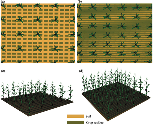
Table 1. Experiment parameters used in LESS model.

Experiment	$f_v$	$f_r$	Solar			Sensor		Soil type	Residue type
			Zenith angle	Azimuth angle	Zenith angle		Azimuth angle
I	0:0.1:0.9	0:0.1:0.9	45	90	0		0	All	Maize, Paddy rice
II	0.3, 0.6	0.6, 0.3	0:10:70	0:30:330	0		0	Phaeozems	Maize

2.3. Sensitivity of vegetation indices to crop residues

To measure variations in VIs due to the presence of crop residues over farmland, we calculated the average bias ($\epsilon$) of VIs as follows:

(1) $\epsilon =\frac{{\sum }_{j=0.1}^{1-i}(V{I}_{f_r=j,f_v=i}-V{I}_{f_r=0,f_v=i})}{N}\left(i=0,0.1,\dots ,0.9\right)$(1)

where $f_v$ and $f_r$ represent the coverage of green crop and crop residue ranging from 0 to 0.9 with a step of 0.1, respectively. $f_v$, $f_r$, and $f_s$ were constrained to sum to unity. $N$ is dependent on the value of j. For example, if$f_v$ is 0.1, there are 10 values of $f_r$ (i.e. 0 ~ 0.9). Then, the value of N is 10.

2.4. DPM and FVC-estimated uncertainty

DPM assumes that the surface of a pixel consists of two parts: vegetation and non-vegetation, and the spectral response of the pixel is the area-averaged reflectance of these two components (Gutman and Ignatov 1998). In order to maximize the difference between vegetation and non-vegetation, VI is commonly used to replace reflectance and it can be represented as:

(2) $\mathrm{V}\mathrm{I}=\mathrm{V}{\mathrm{I}}_{\mathrm{v}}\times \mathrm{F}\mathrm{V}\mathrm{C}+\mathrm{V}{\mathrm{I}}_{\mathrm{s}}\times \left(1-\mathrm{F}\mathrm{V}\mathrm{C}\right)\hspace{0.17em}$(2)

where $\mathrm{V}\mathrm{I}$ refers to the vegetation index of a specific mixed pixel. $\mathrm{V}{\mathrm{I}}_{\mathrm{v}}$ and $\mathrm{V}{\mathrm{I}}_{\mathrm{s}}$ represent the VI values of vegetation and bare soil endmembers, respectively. Therefore, the FVC can be estimated as follows:

(3) $\mathrm{F}\mathrm{V}\mathrm{C}=\frac{\mathrm{V}\mathrm{I}-\mathrm{V}{\mathrm{I}}_{\mathrm{s}}}{\mathrm{V}{\mathrm{I}}_{\mathrm{v}}-\mathrm{V}{\mathrm{I}}_{\mathrm{s}}}\hspace{0.17em}$(3)

Here, we investigated the impact of crop residue on FVC calculation. We calculated an adjusted estimate FVC* by keeping $\mathrm{V}{\mathrm{I}}_{\mathrm{v}}$ and $\mathrm{V}{\mathrm{I}}_{\mathrm{s}}$ constant while varying VI by increasing $f_r$ from 0.1 to 1-i for scenes with a specific $f_v$ equal i. The FVC* can be expressed as:

(4) $\mathrm{F}\mathrm{V}{\mathrm{C}}^{\ast }=\frac{1}{N}\left(\frac{{\sum }_{j=0.1}^{1-i}V{I}_{f_v=i,\hspace{0.17em}{f}_r=j}-\mathrm{V}{\mathrm{I}}_{\mathrm{s}}}{\mathrm{V}{\mathrm{I}}_{\mathrm{v}}-\mathrm{V}{\mathrm{I}}_{\mathrm{s}}}\right)$(4)

The difference between FVC and FVC* was then calculated and hereafter referred to as FVC-estimated error (ΔFVC):

(5) $\mathrm{\Delta }\mathrm{F}\mathrm{V}\mathrm{C}=\mathrm{F}\mathrm{V}{\mathrm{C}}^{\ast }-\mathrm{F}\mathrm{V}\mathrm{C}$(5)

We selected eight VIs which were NDVI, RVI, EVI, normalized difference phenology index (NDPI), soil-adjusted VIs (i.e. PVI, SAVI, TSAVI), and L-SAVI (Table 2). NDPI uses a weighted red-shortwave infrared (SWIR) combination to replace the red band in NDVI (Wang et al. 2017), which can offset the impact of soil background (Xu et al. 2021). A value of L = −0.25 was employed in L-SAVI. Simulated reflectances at 490, 660, 800, 1600, 2000, 2100, and 2200 nm were used to calculate the VIs.

Table 2. Vegetation indices used in this study.

Index	Formula	References
NDVI	$\frac{R_{NIR}-R_{red}}{R_{NIR}+R_{red}}$	Rouse et al. (1974)
RVI	$\frac{R_{NIR}}{R_{red}}$	Pearson and Miller (1972)
EVI	$2.5\times \frac{R_{NIR}-R_{red}}{R_{NIR}+6\times R_{red}-7.5\times R_{blue}+1}$	Liu and Huete (1995)
NDPI	$\frac{R_{NIR}-(0.74\times R_{red}+0.26\times R_{SWIR})}{R_{NIR}+(0.74\times R_{red}+0.26\times R_{SWIR})}$	Wang et al. (2017)
PVI	$\frac{R_{NIR}-a\times R_{red}-b}{\sqrt{1+a^2}}$	Richardson and Wiegand (1977)
SAVI	$\frac{R_{NIR}-R_{red}}{R_{NIR}+R_{red}+0.5}\times 1.5$	Huete (1988)
TSAVI	$\frac{a\times \left(R_{NIR}-a\times R_{red}-b\right)}{a\times R_{NIR}+R_{red}+a\times b}$	Baret, Guyot, and Major (1989)
L-SAVI	$\frac{1.5\times \left(1+L\times \mathrm{C}\mathrm{A}\mathrm{I}\right)\times \left(R_{NIR}-R_{red}\right)}{R_{NIR}+R_{red}+0.5+L\times \mathrm{C}\mathrm{A}\mathrm{I}}$	Ren and Zhou (2014)

$\mathrm{C}\mathrm{A}\mathrm{I}=\hspace{0.17em}100\hspace{0.17em}\times (\frac{R_{2000\hspace{0.17em}nm}+R_{2200\hspace{0.17em}nm}}{2}-R_{2100\hspace{0.17em}nm}$).

3. Results

3.1. Spectral difference between crop residues and soils

The spectral curves of two types of residues and five types of soils are shown in Figure 2. Over the entire wavelength range, the maize residue displayed a higher reflectance than the paddy rice residue (Figure 2(a)). The spectral signatures of the five soils varied in shape and amplitude. In red-NIR wavelengths, the maize residue spectral reflectance was greater than the five soils. The reflectance of paddy rice residue was lower in both bands than Luvisols and Anthrosols, but greater than the other soils. We found both a crop residue line and a soil line in the red-NIR space (Figure 2(b,c)), which is consistent with prior studies (Zhao, Yang, and An 2012; Nagler, Daughtry, and Goward 2000). In order to evaluate the influence of the spectral contrast between residues and soils, PVI and TSAVI were calculated using the soil line (i.e. a = 1.1132, b  = 0.0243).

Figure 2. Spectral reflectance of maize residue, paddy rice residue and five typical soils used in this study.

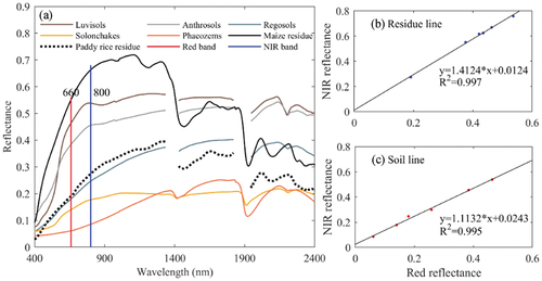
As the majority of the eight VIs in Table 2 were calculated by red and NIR bands, we quantified the spectral absolute difference (AD) between residues and soils as the difference between the spectral sum of crop residue and the spectral sum of soil in red and NIR bands (Table 3). The higher reflectance of maize residue compared to soils contributed to positive ADs (Figure 2). The maize residue had the highest AD (1.06) with Phaeozem soil and the lowest (0.21) with Luvisols. The paddy rice residue had negative ADs with Luvisols and Anthrosols, but had positive ADs with Solonchaks and Phaeozems. Paddy rice residue and Regeosol soil had similar reflectance, resulting in a tiny AD approaching 0. It indicates that AD can detect spectral differences between residues and soils in red and NIR bands.

Table 3. The spectral absolute difference (AD) between crop residues and soils in red and NIR wavelengths.

	Luvisols	Anthrosols	Regosols	Solonchaks	Phaeozems
Maize residue	0.21	0.37	0.79	0.90	1.06
Paddy rice residue	−0.54	−0.37	0.04	0.15	0.32

3.2. Sensitivity of VIs to crop residues

We simulated green crops mixing with two residue types over five soil types in Experiment I, and calculated the canopy VIs listed in Table 2. The responses of VIs with respect to $f_v$ and $f_r$ ranging from 0 to 1.0 over the five types of soils are illustrated in the additional material (Figure S1 and Figure S2). The effects of crop residues on VI were computed using Equation (1)(1) $\epsilon =\frac{{\sum }_{j=0.1}^{1-i}(V{I}_{f_r=j,f_v=i}-V{I}_{f_r=0,f_v=i})}{N}\left(i=0,0.1,\dots ,0.9\right)$(1) and the results are shown in Figures 3 and 4. VIs were affected by the spectral contrast between crop residues and soils in the red-NIR wavelength region, as well as the coverage of crop residues. NDVI was unaffected by changing the maize residue cover over Luvisols and Anthrosols ($\epsilon$ ≈0) (Figure 3(a)). In red and NIR bands, the spectral similarity of the two soils and maize residue (AD = 0.21 and 0.37) resulted in minor NDVI variances. However, combining maize residue with green crops over Regosol, Solonchake, and Phaeozem soils decreased NDVI ($\epsilon$ <0) and caused large deviations. The spectral contrasts among maize residue and these three soils were greater than the spectral contrasts between maize residue and the first two soils, as measured by positive AD values of 0.79, 0.90, and 1.06, respectively. In the case of canopy mixing with paddy rice residues (Figure 3(e)), NDVI values over Luvisols and Anthrosols were greater than no residue treatment readings ($\epsilon$ >0), owing to paddy rice residue’s lower red and NIR reflectance relative to the two soils (ADs <0). When paddy residue cover was changed over Regosols and Solonchaks, there was no obvious difference in NDVI ($\epsilon$ ≈ zero). The ADs between paddy rice residues and these two soils were lower than the ADs between paddy rice residue and other soils (AD = 0.04 and 0.15, respectively). The combination of paddy rice residue and Phaeozems reduced NDVI values and caused larger variations than other soils.

Figure 3. Variations in NDVI, RVI, EVI and NDPI calculated from the reflectances of canopy mixing with maize residue (top row) and paddy rice residue (bottom row) over five soils, with $f_r$ ranging from 0 to 0.9, respectively.

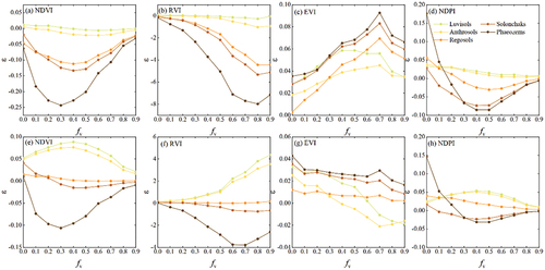
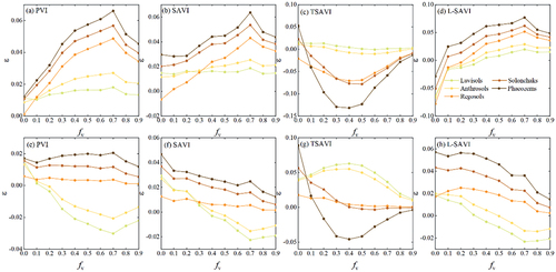
Figure 4. Variations in PVI, SAVI, TSAVI and L-SAVI calculated from the reflectances of canopy mixing with maize residue (top row) and paddy rice residue (bottom row) over five soils with $f_r$ ranging from 0 to 0.9, respectively.

Crop residues produced fluctuations in RVI, too, as shown in Figure 3(b,f). Similar to NDVI, changing maize residue cover over Luvisols and Anthrosols resulted in negligible variations in RVI (Figure 3(b)), but maize residue treatments on the other three soils (ADs >0) resulted in decreased RVI ($\epsilon$ <0), with increasing variation as $f_v$ increased. When compared to the RVI of no residue, paddy rice residue on Luvisols and Anthrosols increased RVI ($\epsilon$ >0) (Figure 3(f)), with greater variance as $f_v$ increased. The absence of difference in RVI was owing to similar reflectances in red and NIR bands among paddy rice residue, Regosols, and Solonchaks. On Phaeozem soil, paddy rice residue treatments reduced RVI.

In terms of EVI (Figure 3(c)), maize residue treatments on all five soils increased EVI ($\epsilon$ >0), with increasing variation as $f_v$ increased, but paddy rice residue had more slight impact on EVI regardless of soil (−0.02 < $\epsilon$ <0.05). Over Luvisols and Anthrosols (ADs <0), EVI decreased when $f_v$ was greater than 0.4 and 0.6, respectively (Figure 3(g)). EVI was less sensitive to crop residues in comparison with NDVI and RVI. For both residues, NDPI, which was meant to minimize the impact of the soil background (Wang et al. 2017), exhibited similar patterns to NDVI (Figure 3(d,h)). When $f_v$ was zero, the NDPI value for Phaeozem soil was less than zero (−0.112), resulting in a large bias as $f_r$ changed. The treatments with residues over Solonchaks and Phaeozems resulted in reduced NDPI, while the finding was reversed for Luvisols and Anthrosols.

Figure 4 shows the responses of PVI, SAVI, TSAVI, and L-SAVI to changes in $f_r$ on soils. Variations in PVI, SAVI, and L-SAVI caused by maize residue cover were similar to those in the EVI (Figure 4(a,c,d)). PVI, SAVI, and L-SAVI all increased in response to changes in maize residue cover, and their variations peaked at $f_v$ around 0.7. When paddy rice residue was mixed with green crops over Luvisols and Anthrosols, PVI, SAVI, and L-SAVI all decreased when $f_v$ was greater than 0.2, 0.4, and 0.5, respectively (Figure 4(e,f,h)). PVI, SAVI, and L-SAVI increased as residue was present in the other three soils that had positive ADs with paddy rice residue. These three indices were less affected paddy rice residues than maize residues. For TSAVI, changes in TSAVI caused by crop residue cover were similar to those of NDVI (Figure 4(c,g)).

To summarize, crop residue in the canopy induced changes in the above VIs. The responses of VIs to crop residues were strongly affected by the spectral contrast between crop residues and soils. EVI, PVI, SAVI, and L-SAVI were less affected by crop residues in comparison with NDVI, RVI, and TSAVI. NDPI demonstrated the potential to reduce the impact of crop residues.

3.3. Uncertainty of FVC caused by crop residue

Figures 5 and 6 illustrate the FVC-estimated error ($\mathrm{\Delta }\mathrm{F}\mathrm{V}\mathrm{C}$) between FVC derived from Equation (3)(3) $\mathrm{F}\mathrm{V}\mathrm{C}=\frac{\mathrm{V}\mathrm{I}-\mathrm{V}{\mathrm{I}}_{\mathrm{s}}}{\mathrm{V}{\mathrm{I}}_{\mathrm{v}}-\mathrm{V}{\mathrm{I}}_{\mathrm{s}}}\hspace{0.17em}$(3) and FVC* derived from Equation (4)(4) $\mathrm{F}\mathrm{V}{\mathrm{C}}^{\ast }=\frac{1}{N}\left(\frac{{\sum }_{j=0.1}^{1-i}V{I}_{f_v=i,\hspace{0.17em}{f}_r=j}-\mathrm{V}{\mathrm{I}}_{\mathrm{s}}}{\mathrm{V}{\mathrm{I}}_{\mathrm{v}}-\mathrm{V}{\mathrm{I}}_{\mathrm{s}}}\right)$(4) . When maize residue was mixed with green crops, the decrease in NDVI and RVI caused by maize residue resulted in underestimation of FVC by these VI-based DPMs across all soils (Figure 5(a,b)). The NDVI-based model was particularly sensitive to the spectral difference between maize residue and soil, especially with low vegetation cover ($f_v$ = 0.3: $\mathrm{\Delta }\mathrm{F}\mathrm{V}\mathrm{C}$ over Regolos = −0.14, AD = 0.79; $\mathrm{\Delta }\mathrm{F}\mathrm{V}\mathrm{C}$ over Solonchakes = −0.15, AD = 0.90; $\mathrm{\Delta }\mathrm{F}\mathrm{V}\mathrm{C}$ over Phaeozems = −0.32, AD = 1.06). Compared to NDVI-based model, the $\mathrm{\Delta }\mathrm{F}\mathrm{V}\mathrm{C}$ obtained with the RVI-based model was lower under low vegetation cover ($f_v$ <0.5); however, the underestimation increased with $f_v$. The underestimation also increased as the AD values increased. The EVI-based model overestimated FVC but outperformed the NDVI- and RVI-based models ($\mathrm{\Delta }\mathrm{F}\mathrm{V}\mathrm{C}$ was below 0.1). The NDPI-based model underestimated under medium vegetation cover ($f_v$ = 0.3 ~ 0.7) over Solonchaks and Phaeozems. The EVI- and NDPI-based models were less affected by maize residue.

Figure 5. $\mathrm{\Delta }\mathrm{F}\mathrm{V}\mathrm{C}$ between FVC* and FVC caused by the presence of maize residue (top row) and paddy rice residue (bottom row) derived from NDVI-, RVI-, EVI- and NDPI-based models over five soils.

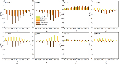
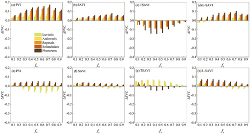
Figure 6. $\mathrm{\Delta }\mathrm{F}\mathrm{V}\mathrm{C}$ between FVC* and FVC caused by the presence of maize residue (top row) and paddy rice residue (bottom row) derived from PVI-, SAVI-, TSAVI- and L-SAVI-based models over five soils.

In comparison with maize residue, paddy rice residue had a lower impact on the four models across different soils (Figure 5(e–h)). The NDVI- and RVI-based models both overestimated over Luvisols and Anthrosols and underestimated over Phaeozems (Figure 5(e–f)). Paddy rice residue covered on Regosols and Solonchakes had little influence on these two models. The $\mathrm{\Delta }\mathrm{F}\mathrm{V}\mathrm{C}$ of the EVI-based model was negligible across all soils. The NDPI-based model generally overestimated under low and medium vegetation cover ($f_v$ = 0.3 ~ 0.7) over the first three soils.

Figure 6 shows the $\mathrm{F}\mathrm{V}\mathrm{C}$ derived from the PVI-, SAVI-, TSAVI-, and L-SAVI-based models. When green crops were mixed with maize residue, the increase in PVI, SAVI, and L-SAVI led to overestimation of FVC by these VI-based DPMs. These models performed similarly to the EVI-based model and followed the same trend as soil changed (Figure 6(a,b,d)). The TSAVI-based model underestimated, performing similarly to the NDVI-based model (Figure 6(c)). The PVI-, SAVI-, and L-SAVI-based models were less affected by paddy rice residue (−0.1 < $\mathrm{\Delta }\mathrm{F}\mathrm{V}\mathrm{C}$ <0.1) (Figure 6(e,f,h)). The TSAVI-based model performed similarly to the NDVI-based model, but with lower $\mathrm{\Delta }\mathrm{F}\mathrm{V}\mathrm{C}$ values (Figure 6(g)). SAVI outperformed the other three VI-based models, followed by the L-SAVI-based model.

Overall, FVC was overestimated or underestimated when crop residues were present with green crops. Of the eight VI-based models, the EVI-, NDPI, SAVI-, and L-SAVI-based models were less affected by crop residues. Despite the fact that TSAVI and PVI included soil line parameters, models based on these indices produced higher $\mathrm{\Delta }\mathrm{F}\mathrm{V}\mathrm{C}$ than EVI-, NDPI, and SAVI-based models. NDVI- and RVI-based models were most affected by crop residues.

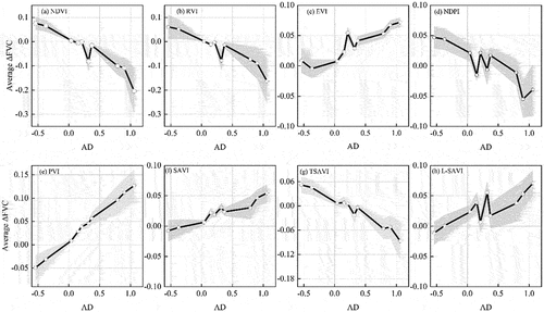
The plots of AD values (Table 3) and the averaged $\mathrm{\Delta }\mathrm{F}\mathrm{V}\mathrm{C}$ calculated from each VI-based model are presented in Figure 7. The averaged $\mathrm{\Delta }\mathrm{F}\mathrm{V}\mathrm{C}$ obtained from NDVI-, RVI-, NDPI, and TSAVI-based models decreased with AD values (Figure 7(a,b,d,g)). When the AD was less than 0, the averaged $\mathrm{\Delta }\mathrm{F}\mathrm{V}\mathrm{C}$ calculated by these models was negative, but as the AD increased, it became positive. The averaged $\mathrm{\Delta }\mathrm{F}\mathrm{V}\mathrm{C}$ estimated by NDVI- and RVI-based models ranged between −0.3 and 0.1. With increasing AD values, there was a trend towards increasing averaged $\mathrm{\Delta }\mathrm{F}\mathrm{V}\mathrm{C}$ obtained from EVI-, PVI-, SAVI, and L-SAVI-based models (Figure 7(c,e,f,h)). The averaged $\mathrm{\Delta }\mathrm{F}\mathrm{V}\mathrm{C}$ obtained by EVI- and SAVI-based models ranged between around 0 and 0.1. These results indicated that the overestimation or underestimation of FVC caused by crop residues can be qualitatively determined by AD values.

Figure 7. AD values and averaged $\mathrm{F}\mathrm{V}\mathrm{C}$ calculated from the eight VI-based models over different soils.

3.4. Influence of the solar position

In Experiment II, we studied the influence of solar position on DPM models. The shadow areas of green crops, maize residues, and soil increased with SZA (Figure 8). Variations in $\mathrm{\Delta }FVC$ in response to changes in SZA and SAA are shown in Figure 9. The $\mathrm{\Delta }FVC$ calculated by the EVI-, SAVI-, TSAVI-, and L-SAVI-based models changed with SZA and SAA when $f_v$ and $f_r$ of the simulated scene were 0.3 and 0.6 (Figure 9(a)). The $\mathrm{\Delta }FVC$ of the EVI- and L-SAVI-based models increased with SZA along the diagonal directions. The NDVI-, RVI- and NDPI-based models were less affected by solar angle. The $\mathrm{\Delta }FVC$ derived from PVI-based model decreased with SZA. When $f_v$ and $f_r$ of the simulated scene were 0.6 and 0.3 (Figure 9(b)), the distribution of $FVC$ for each VI-based model changed except for the NDPI-and TSAVI-based models. The $FVC$ of the EVI-, SAVI-, and L-SAVI-based models increased with SZA along the diagonal directions. The PVI-based model was not sensitive to SAA. The NDVI- and RVI-based models became more sensitive to solar position as $f_v$ increased.

Figure 8. Variations in the six-component ratio as a function of SZA: (a) $f_v$ = 0.3 $f_r$ =0.6; (b) $f_v$ = 0.6, $f_r$ = 0.3.

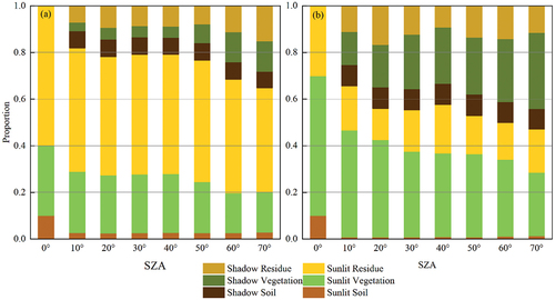
Figure 9. The responses of $\mathrm{\Delta }FVC$ to changes in solar position for two canopies with different coverages of green crops and maize residues: (a) $f_v$ = 0.3 $f_r$ =0.6; (b) $f_v$ = 0.6, $f_r$ = 0.3.

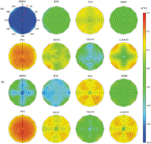
In general, the NDPI-based model was least affected by the solar position, followed by the PVI- and TSAVI-based models. EVI-, SAVI, and L-SAVI models were more sensitive to SZA in the diagonal directions. Under low vegetation cover, models based on NDVI and RVI were less affected by SZA.

4. Discussion

4.1. Impact of crop residue on VIs

The spectral characteristics of crop residue depend on lignin and cellulose content, crop types, moisture content, degree of decomposition and so on (Daughtry et al. 1996.; Wang et al. 2013). As moisture content and degree of decomposition increase, the reflectance of crop residue across all wavelengths decreases (Quemada and Daughtry 2016). Soil reflectance is influenced by organic matter content, surface roughness, texture, and moisture (Ge et al. 2011; Rossel et al. 2016). As a result, the residue reflectance in the VIS-NIR wavelengths may be higher or lower than soil reflectance. In order to address the spectral difference between crop residue and soil, we selected two types of residues and five typical soils, and we successfully used AD to measure the differences between them in red and NIR bands. Among these, paddy rice residue had a higher or lower reflectance than the five soils, resulting in AD values that were either positive or negative. Since the selected maize residue showed a higher reflectance than the five soils, all AD values were all positive.

The higher or lower reflectance of crop residues relative to soils in red and NIR bands resulted in increases or decreases in VIs when crop residues were mixed with green crops. The paddy rice residue used by Zhao, Yang, and An (2012) had a higher red and NIR reflectance than the soil, leading them to conclude that changing the background from bare soil to rice residue reduced NDVI, RVI, and TSAVI. Our findings corroborate the result. Moreover, we found that when crop residue had a higher red and NIR reflectance than soil, EVI, PVI, SAVI, and L-SAVI increased, and when the reflectance of crop residue was lower than soil, these four VIs decreased under medium and high vegetation cover. Among the eight VIs we selected, NDVI and RVI were highly sensitive to the spectral contrast between crop residue and soil, which was also reported by Zhao, Yang, and An (2012). Although TSAVI incorporates soil line information, it hardly reduced the impact of crop residue. EVI gained its heritage from SAVI (Jiang et al. 2008), and effectively minimized the impact of crop residue. NDPI was less sensitive to dry matter in comparison with NDVI and RVI (Xu et al. 2021), which was also found less affected by crop residue. SAVI, incorporating the soil adjusted factor L, successfully resisted crop residue. These VIs could be used to estimate FVC and other biophysical parameters from low-tilled cropland such as leaf area index. We supported Ren and Zhou (2014)’s findings that L-SAVI lessens the impact of crop residue. However, the CAI as an adjusted factor used in the L-SAVI is a hyperspectral index (Nagler et al. 2003). The application of L-SAVI would be limited by the available hyperspectral sensor in orbit.

4.2. Limits of the DPM

The DPM assumes that the surface of a pixel is composed of vegetation and non-vegetation (Gutman and Ignatov 1998). Although the assumption does not hold in real scenarios such as conservation tillage farmland and grassland (Xu, An, and Guo 2020; Zheng, Campbell, and de Beurs 2012), few studies have evaluated the effect of neglecting crop residue (or plant litter). Therefore, we employed VI-based DPMs to investigate. The responses of VIs to crop residue directly influenced the performance of VI-based DPMs (Figures 5 and 6). Previous studies have found that NDVI- and RVI-based models are sensitive to soil brightness (Yan et al. 2021; Huete and Jackson 1988). In the present study, these two models were most affected by crop residue due to the sensitivities of NDVI and RVI to crop residue. The first three models with the lowest $\mathrm{F}\mathrm{V}\mathrm{C}$ were SAVI-, EVI-, and L-SAVI-based models. We found that $\mathrm{F}\mathrm{V}\mathrm{C}$ was highly correlated to the AD values between crop residues and soils (Figure 7). Furthermore, we discovered that the bias of the NDPI-based model was minimally changed with SZA. We therefore concluded that NDPI was least sensitive to shadow. After comprehensive comparison, the EVI-, SAVI-, L-SAVI and NDPI-based models are recommended. However, it should be noted that the accuracies of VI-based DPMs on estimating FVC was not explored in this study. Yan et al. (2021) and Ding et al. (2017) compared the performance of a series of VI-based DPMs on FVC estimation based on simulation data and field measurements, respectively.

Currently, a triangle space method is used to simultaneously estimate FVC and CRC (Yue et al. 2020), which assumes that the NDVI of a pixel is the linear combination of the NDVI of three endmembers (green crops, crop residue, and soil) weighted by their percent covers and the CAI of the pixel is the linear combination of the CAI of three endmembers (Guerschman et al. 2009). The model forces the proportions of the three components to sum to unity. As a result, the CRC and FVC can be calculated. However, the present study and Zhao, Yang, and An (2012) demonstrated that NDVI is sensitive to crop residues. Serbin et al. (2009) and Dennison et al. (2019) found that CAI is sensitive to green vegetation. Therefore, the application of the triangle space method should consider how to reduce the interaction between vegetation and crop residues. Based on this study, EVI, SAVI, L-SAVI, and NDPI are recommended to replace NDVI in the triangle space method. Besides, multiple endmember spectral mixture analysis (MESMA) has been used to estimate FVC from mixed pixel containing multiple endmembers (Meyer and Okin 2015).

4.3. Limitations and implications

The impact of crop residue was investigated using simulation data, so further quantitative validation from field sites is necessary. Moreover, this study only investigated the retrieval of FVC. Nevertheless, the estimation of other crop biophysical parameters (e.g. leaf area index and canopy chlorophyll content) would be also impacted by crop residue. Future research could involve more efforts towards developing new VIs less sensitive to crop residue. Recently, the red edge (RE) (680–780 nm) indices were found to be favourable for monitoring biophysical parameters of plants (Dong et al. 2019; Deng et al. 2021; Hu et al. 2020). RE bands may help reduce the noise of crop residue, which have been found to be less sensitive to the soil background (Liu et al. 2022; Hu et al. 2020). The potential of RE information to improve the estimation of crop information is worth exploring further. Moreover, the spectral difference between crop residue and soil can be better captured by hyperspectral bands and there is no doubt that crop variables can be estimated with improved accuracy by hyperspectral data. New-generation imaging spectrometer missions include PRISMA (Loizzo et al. 2018) and EnMAP (Guanter et al. 2015) which cover contiguous narrow bands. It is expected that these hyperspectral missions could enable an improved retrieval of crop biophysical information over low-tilled cropland.

5. Conclusion

This study investigated the effect of crop residue on VIs and VI-based DPMs using simulated reflectance from the LESS model. The spectral discrepancy between crop residue and soil in red and NIR bands was effectively measured by AD. The presence of crop residue having negative AD with soils contributed to increases in NDVI, RVI, TSAVI, and NDPI and decreases in EVI, PVI, SAVI, L-SAVI under medium and high vegetation cover. NDVI, RVI, TSAVI, and NDPI decreased whereas other VIs increased with the presence of crop residue that having positive ADs with soils. EVI- and SAVI-based DPMs effectively reduced the effect of crop residue with FVC-estimation uncertainty lower than 0.1, followed by the NDPI- and L-SAVI-based models, while the NDVI and RVI-based model performed poorly. The FVC-estimated uncertainty of each VI-based DPM was highly correlated to AD values. Moreover, solar position increased the uncertainty of VI-based DPMs due to appearance of shadow area. The NDPI-based model was least affected by solar position. Our results revealed that crop residue had an impact on VIs and the retrieval of FVC from VIs. Further research needs to consider the impact of crop residue when estimating crop biophysical parameters over low-tilled cropland.

Disclosure statement

No potential conflict of interest was reported by the authors.

Supplementary material

Supplemental data for this article can be accessed online at https://doi.org/10.1080/01431161.2022.2139649.

Additional information

Funding

This study was supported by the National Natural Science Foundation of China [number 42271333], and the Natural Science Foundation of Jilin Province (The central government guides local science and technology development funds) [number YDZ202201ZYTS484], the Strategic Priority Research Program of the Chinese Academy of Sciences under Grant [number XDA28070500], Fundamental Research Funds of for the Central Universities under Grant [number 2412020FZ004], Land Observation Satellite Supporting Platform of National Civil Space Infrastructure Project under Grant [CASPLOS-CCSI], the Science and Technology Project of the Department of Education, Jilin Province under Grant [JJKH20221163K].

References

- Baret, F., G. Guyot, and D. J. Major. 1989. “TSAVI: A Vegetation Index Which Minimizes Soil Brightness Effects on LAI and APAR Estimation.” Paper presented at the 12th IEEE Canadian Symposium on Remote Sensing Geoscience and Remote Sensing Symposium. Vancouver, Canada.
- CTIC. 2004. National Survey of Conservation Tillage Practices. West Lafayette, IN: Conservation Technology Information Center.
- Daughtry, C. S. T., and E. R. Hunt. 2008. “Mitigating the Effects of Soil and Residue Water Contents on Remotely Sensed Estimates of Crop Residue Cover.” Remote Sensing of Environment 112 (4): 1647–1657. doi:10.1016/j.rse.2007.08.006.
- Daughtry, C. S. T., J. E. McMurtrey III, P. L. Nagler, M. S. Kim, and E. W. Chappelle. 1996. Spectral reflectance of soils and crop residues. Near Infrared Spectroscopy: The Future Waves. Chichester,UK: NIR Publictions.
- Deng, Z. D., Z. Lu, G. Y. Wang, D. Q. Wang, Z. B. Ding, H. F. Zhao, H. L. Xu, Y. Shi, Z. J. Cheng, and X. N. Zhao. 2021. “Extraction of Fractional Vegetation Cover in Arid Desert Area Based on Chinese GF-6 Satellite.” Open Geosciences 13 (1): 416–430. doi:10.1515/geo-2020-0241.
- Dennison, P. E., Y. Qi, S. K. Meerdink, R. F. Kokaly, D. R. Thompson, C. S. T. Daughtry, M. Quemada, et al. 2019. ”Comparison of Methods for Modeling Fractional Cover Using Simulated Satellite Hyperspectral Imager Spectra.” Remote Sensing 11 (18): 2072. doi:10.3390/rs11182072.
- Derpsch, R., T. Friedrich, A. Kassam, and H. W. Li. 2010. “Current Status of Adoption of No-Till Farming in the World and Some of Its Main Benefits.” International Journal of Agricultural and Biological Engineering 3 (1): 1–25. doi:10.3965/j.issn.1934-6344.2010.01.001-025.
- Diepen, C. A., J. Wolf, H. Keulen, and C. Rappoldt. 1989. “WOFOST: A Simulation Model of Crop Production.” Soil Use and Management 5 (1): 16–24. doi:10.1111/j.1475-2743.1989.tb00755.x.
- Ding, Y. L., H. Y. Zhang, K. Zhao, and X. M. Zheng. 2017. “Investigating the Accuracy of Vegetation Index-Based Models for Estimating the Fractional Vegetation Cover and the Effects of Varying Soil Backgrounds Using in situ Measurements and the PROSAIL Model.” International Journal of Remote Sensing 38 (14): 4206–4223. doi:10.1080/01431161.2017.1312617.
- Ding, Y. L., X. M. Zheng, K. Zhao, X. P. Xin, and H. J. Liu. 2016. “Quantifying the Impact of NDVIsoil Determination Methods and NDVIsoil Variability on the Estimation of Fractional Vegetation Cover in Northeast China.” Remote Sensing 8 (1): 29. doi:10.3390/rs8010029.
- Dong, T. F., J. G. Liu, J. L. Shang, B. D. Qian, B. L. Ma, J. M. Kovacs, D. Walters, X. F. Jiao, X. Y. Geng, and Y. C. Shi. 2019. “Assessment of Red-Edge Vegetation Indices for Crop Leaf Area Index Estimation.” Remote Sensing of Environment 222: 133–143. doi:10.1016/j.rse.2018.12.032.
- Ge, Y. F., C. L. S. Morgan, S. Grunwald, D. J. Brown, and D. V. Sarkhot. 2011. “Comparison of Soil Reflectance Spectra and Calibration Models Obtained Using Multiple Spectrometers.” Geoderma 161 (3–4): 202–211. doi:10.1016/j.geoderma.2010.12.020.
- Govaerts, Y. M., and M. M. Verstraete. 1998. “Raytran: A Monte Carlo Ray-Tracing Model to Compute Light Scattering in Three-Dimensional Heterogeneous Media.” IEEE Transactions on Geoscience and Remote Sensing 36 (2): 493–505. doi:10.1109/36.662732.
- Guanter, L., H. Kaufmann, K. Segl, S. Foerster, C. Rogass, S. Chabrillat, T. Kuester, et al. 2015. ”The EnMap Spaceborne Imaging Spectroscopy Mission for Earth Observation.” Remote Sensing 7 (7): 8830–8857. doi:10.3390/rs70708830.
- Guerschman, J. P., M. J. Hill, L. J. Renzullo, D. J. Barrett, A. S. Marks, and E. J. Botha. 2009. “Estimating Fractional Cover of Photosynthetic Vegetation, Non-Photosynthetic Vegetation and Bare Soil in the Australian Tropical Savanna Region Upscaling the EO-1 Hyperion and MODIS Sensors.” Remote Sensing of Environment 113 (5): 928–945. doi:10.1016/j.rse.2009.01.006.
- Gutman, G., and A. Ignatov. 1998. “The Derivation of the Green Vegetation Fraction from NOAA/AVHRR Data for Use in Numerical Weather Prediction Models.” International Journal of Remote Sensing 19 (8): 1533–1543. doi:10.1080/014311698215333.
- He, Y., X. L. Guo, and J. Wilmshurst. 2006. “Studying Mixed Grassland Ecosystems I: Suitable Hyperspectral Vegetation Indices.” Canadian Journal of Remote Sensing 32 (2): 98–107. doi:10.5589/m06-009.
- Hsiao, T. C., L. Heng, P. Steduto, B. Rojas‐lara, D. Raes, and E. Fereres. 2009. “AquaCrop—the FAO Crop Model to Simulate Yield Response to Water: III. Parameterization and Testing for Maize.” Agronomy Journal 101 (3): 448–459. doi:10.2134/agronj2008.0218s.
- Huete, A. R. 1988. “A Soil-Adjusted Vegetation Index (SAVI).” Remote Sensing of Environment 25 (3): 295–309. doi:10.1016/0034-4257(88)90106-x.
- Huete, A. R., and R. D. Jackson. 1988. “Soil and Atmosphere Influences on the Spectra of Partial Canopies.” Remote Sensing of Environment 25 (1): 89–105. doi:10.1016/0034-4257(88)90043-0.
- Huggins, D. R., and J. P. Reganold. 2008. “No-Till: The Quiet Revolution.” Scientific American 299 (1): 70–77. doi:10.1038/scientificamerican0708-70.
- Hunt, E. R., C. S. T. Daughtry, S. B. Mirsky, and W. D. Hively. 2014. “Remote Sensing with Simulated Unmanned Aircraft Imagery for Precision Agriculture Applications.” IEEE Journal of Selected Topics in Applied Earth Observations and Remote Sensing 7 (11): 4566–4571. doi:10.1109/Jstars.2014.2317876.
- Hu, Q., J. Y. Yang, B. D. Xu, J. X. Huang, M. S. Memon, G. F. Yin, Y. L. Zeng, J. Zhao, and K. Liu. 2020. “Evaluation of Global Decametric-Resolution LAI, FAPAR and FVC Estimates Derived from Sentinel-2 Imagery.” Remote Sensing 12 (6): 912. doi:10.3390/rs12060912.
- Jacquemoud, S., W. Verhoef, F. Baret, C. Bacour, P. J. Zarco-Tejada, G. P. Asner, C. Francois, and S. L. Ustin. 2009. “PROSPECT Plus SAIL Models: A Review of Use for Vegetation Characterization.” Remote Sensing of Environment 113: S56–66. doi:10.1016/j.rse.2008.01.026.
- Jia, K., S. L. Liang, S. H. Liu, Y. W. Li, Z. Q. Xiao, Y. J. Yao, B. Jiang, et al. 2015. ”Global Land Surface Fractional Vegetation Cover Estimation Using General Regression Neural Networks from MODIS Surface Reflectance.” IEEE Transactions on Geoscience and Remote Sensing 53 (9): 4787–4796. doi:10.1109/Tgrs.2015.2409563.
- Jiang, Z. Y., A. R. Huete, J. Chen, Y. H. Chen, J. Li, G. J. Yan, and X. Y. Zhang. 2006. “Analysis of NDVI and Scaled Difference Vegetation Index Retrievals of Vegetation Fraction.” Remote Sensing of Environment 101 (3): 366–378. doi:10.1016/j.rse.2006.01.003.
- Jiang, Z., A. Huete, K. Didan, and T. Miura. 2008. “Development of a Two-Band Enhanced Vegetation Index Without a Blue Band.” Remote Sensing of Environment 112 (10): 3833–3845. doi:10.1016/j.rse.2008.06.006.
- Jiapaer, G., X. Chen, and A. M. Bao. 2011. “A Comparison of Methods for Estimating Fractional Vegetation Cover in Arid Regions.” Agricultural and Forest Meteorology 151 (12): 1698–1710. doi:10.1016/j.agrformet.2011.07.004.
- Jones, J. R., C. S. Fleming, K. Pavuluri, M. M. Alley, M. S. Reiter, and W. E. Thomason. 2015. “Influence of Soil, Crop Residue, and Sensor Orientations on NDVI Readings.” Precision Agriculture 16 (6): 690–704. doi:10.1007/s11119-015-9402-0.
- Li, F., W. Chen, Y. Zeng, Q. J. Zhao, and B. F. Wu. 2014. “Improving Estimates of Grassland Fractional Vegetation Cover Based on a Pixel Dichotomy Model: A Case Study in Inner Mongolia, China.” Remote Sensing 6 (6): 4705–4722. doi:10.3390/rs6064705.
- Li, L. Y., X. H. Mu, C. Macfarlane, W. J. Song, J. Chen, K. Yan, and G. J. Yan. 2018. “A Half-Gaussian Fitting Method for Estimating Fractional Vegetation Cover of Corn Crops Using Unmanned Aerial Vehicle Images.” Agricultural and Forest Meteorology 262: 379–390. doi:10.1016/j.agrformet.2018.07.028.
- Liu, J. L., J. R. Fan, C. Yang, F. B. Xu, X. Y. Zhang, Z. Zhao, W. Jin, W. Shen, and W. Liu. 2022. “Illuminated Border: Spatiotemporal Analysis of COVID-19 Pressure in the Sino-Burma Border from the Perspective of Nighttime Light.” International Journal of Applied Earth Observation and Geoinformation 109. doi:10.1016/j.jag.2022.102793.
- Liu, H. Q., and A. Huete. 1995. ”A feedback based modification of the NDVI to minimize canopy background and atmospheric noise.” IEEE Transactions on Geoscience and Remote Sensing 33 (2):457–65. doi:10.1109/tgrs.1995.8746027.
- Loizzo, R., R. Guarini, F. Longo, T. Scopa, R. Formaro, C. Facchinetti, and G. Varacalli. 2018. “PRISMA: The Italian Hyperspectral Mission.” Paper presented at the IGARSS 2018-2018 IEEE International Geoscience and Remote Sensing Symposium, Valencia, Spain.
- Matese, A., P. Toscano, S. F. Di Gennaro, L. Genesio, F. P. Vaccari, J. Primicerio, C. Belli, A. Zaldei, R. Bianconi, and B. Gioli. 2015. “Intercomparison of UAV, Aircraft and Satellite Remote Sensing Platforms for Precision Viticulture.” Remote Sensing 7 (3): 2971–2990. doi:10.3390/rs70302971.
- Meyer, T., and G. S. Okin. 2015. “Evaluation of Spectral Unmixing Techniques Using MODIS in a Structurally Complex Savanna Environment for Retrieval of Green Vegetation, Nonphotosynthetic Vegetation, and Soil Fractional Cover.” Remote Sensing of Environment 161: 122–130. doi:10.1016/j.rse.2015.02.013.
- Montandon, L., and E. Small. 2008. “The Impact of Soil Reflectance on the Quantification of the Green Vegetation Fraction from NDVI.” Remote Sensing of Environment 112 (4): 1835–1845. doi:10.1016/j.rse.2007.09.007.
- Nagler, P. L., C. S. T. Daughtry, and S. N. Goward. 2000. “Plant Litter and Soil Reflectance.” Remote Sensing of Environment 71 (2): 207–215. doi:10.1016/s0034-4257(99)00082-6.
- Nagler, P. L., Y. Inoue, E. P. Glenn, A. L. Russ, and C. S. T. Daughtry. 2003. “Cellulose Absorption Index (CAI) to Quantify Mixed Soil–Plant Litter Scenes.” Remote Sensing of Environment 87 (2–3): 310–325. doi:10.1016/j.rse.2003.06.001.
- North, P. R. J. 1996. “Three-Dimensional Forest Light Interaction Model Using a Monte Carlo Method.” IEEE Transactions on Geoscience and Remote Sensing 34 (4): 946–956. doi:10.1109/36.508411.
- Pearson, R. L., and L. D. Miller . 1972. ”Remote Mapping of Standing Crop Biomass for Estimation of Productivity of the Shortgrass Prairie.” Remote sensing of environment, VIII:1355.
- Pu, J. B., K. Yan, G. H. Zhou, Y. Q. Lei, Y. X. Zhu, D. H. Guo, H. L. Li, L. L. Xu, Y. Knyazikhin, and R. B. Myneni. 2020. “Evaluation of the MODIS LAI/FPAR Algorithm Based on 3D-RTM Simulations: A Case Study of Grassland.” Remote Sensing 12 (20): 3391. doi:10.3390/rs12203391.
- Qi, J. B., D. H. Xie, T. G. Yin, G. J. Yan, J. P. Gastellu-Etchegorry, L. Y. Li, W. M. Zhang, X. H. Mu, and L. K. Norford. 2019. “LESS: LargE-Scale Remote Sensing Data and Image Simulation Framework Over Heterogeneous 3D Scenes.” Remote Sensing of Environment 221: 695–706. doi:10.1016/j.rse.2018.11.036.
- Quemada, M., and C. S. T. Daughtry. 2016. “Spectral Indices to Improve Crop Residue Cover Estimation Under Varying Moisture Conditions.” Remote Sensing 8 (8). doi:10.3390/rs8080660.
- Ren, H. R., and G. S. Zhou. 2014. “Determination of Green Aboveground Biomass in Desert Steppe Using Litter-Soil-Adjusted Vegetation Index.” European Journal of Remote Sensing 47 (1): 611–625. doi:10.5721/EuJRS20144734.
- Richardson, A. J., and C. L. Wiegand. 1977. “Distinguishing Vegetation from Soil Background Information.” Photogrammetric Engineering Remote Sensing 43 (12): 1541–1552.
- Rossel, R. A. V., T. Behrens, E. Ben-Dor, D. J. Brown, J. A. M. Dematte, K. D. Shepherd, Z. Shi, et al. 2016. ”A Global Spectral Library to Characterize the World’s Soil.” Earth-Science Reviews 155: 198–230. doi:10.1016/j.earscirev.2016.01.012.
- Rouse, J., R. Haas, J. Schell, and D. Deering. 1974. ”Monitoring Vegetation Systems in the Great Plains with ERTS.” NASA Special Publication 1 (24):309–17.
- Serbin, G., C. S. T. Daughtry, E. R. Hunt, D. J. Brown, and G. W. McCarty. 2009. “Effect of Soil Spectral Properties on Remote Sensing of Crop Residue Cover.” Soil Science Society of America Journal 73 (5): 1545–1558. doi:10.2136/sssaj2008.0311.
- Singh, R., M. Serawat, A. Singh, and Babli. 2018. “Effect of Tillage and Crop Residue Management on Soil Physical Properties.” Journal of Soil Salinity and Water Quality 10 (2): 200–206.
- Turmel, M. S., A. Speratti, F. Baudron, N. Verhulst, and B. Govaerts. 2015. “Crop Residue Management and Soil Health: A Systems Analysis.” Agricultural Systems 134: 6–16. doi:10.1016/j.agsy.2014.05.009.
- Van Leeuwen, W. J. D., and A. R. Huete. 1996. “Effects of Standing Litter on the Biophysical Interpretation of Plant Canopies with Spectral Indices.” Remote Sensing of Environment 55 (2): 123–138. doi:10.1016/0034-4257(95)00198-0.
- Wang, C., J. Chen, J. Wu, Y. H. Tang, P. J. Shi, T. A. Black, and K. Zhu. 2017. “A Snow-Free Vegetation Index for Improved Monitoring of Vegetation Spring Green-Up Date in Deciduous Ecosystems.” Remote Sensing of Environment 196: 1–12. doi:10.1016/j.rse.2017.04.031.
- Wang, C. K., X. Z. Pan, Y. Liu, Y. L. Li, R. J. Shi, R. Zhou, and X. L. Xie. 2013. “Alleviating Moisture Effects on Remote Sensing Estimation of Crop Residue Cover.” Agronomy Journal 105 (4): 967–976. doi:10.2134/agronj2012.0460.
- Widlowski, J. L., C. Mio, M. Disney, J. Adams, I. Andredakis, C. Atzberger, J. Brennan, et al. 2015. ”The Fourth Phase of the Radiative Transfer Model Intercomparison (RAMI) Exercise: Actual Canopy Scenarios and Conformity Testing.” Remote Sensing of Environment 169: 418–437. doi:10.1016/j.rse.2015.08.016.
- Xu, D. D., D. S. An, and X. L. Guo. 2020. “The Impact of Non-Photosynthetic Vegetation on LAI Estimation by NDVI in Mixed Grassland.” Remote Sensing 12 (12). doi:10.3390/rs12121979.
- Xu, D. W., C. Wang, J. Chen, M. G. Shen, B. B. Shen, R. R. Yan, Z. W. Li, et al. 2021. ”The Superiority of the Normalized Difference Phenology Index (NDPI) for Estimating Grassland Aboveground Fresh Biomass.”Remote Sensing of Environment 264.doi:10.1016/j.rse.2021.112578.
- Yan, K., S. Gao, H. J. Chi, J. B. Qi, W. J. Song, Y. Y. Tong, X. H. Mu, and G. J. Yan. 2021. “Evaluation of the Vegetation-Index-Based Dimidiate Pixel Model for Fractional Vegetation Cover Estimation.” IEEE Transactions on Geoscience and Remote Sensing 60: 1–14. doi:10.1109/tgrs.2020.3048493.
- Yang, Y. Y., T. X. Wu, S. D. Wang, and H. Li. 2020. “Fractional Evergreen Forest Cover Mapping by MODIS Time-Series FEVC-CV Methods at Sub-Pixel Scales.” ISPRS Journal of Photogrammetry and Remote Sensing 163: 272–283. doi:10.1016/j.isprsjprs.2020.03.012.
- Yue, J. B., Q. J. Tian, X. Y. Dong, N. X. Xu, J. Wu, N. Pavlovic, C. Breton, F. Gilliland, and R. Habre. 2020. “Spatiotemporal Imputation of MAIAC AOD Using Deep Learning with Downscaling.” Remote Sensing of Environment 237. doi:10.1016/j.rse.2019.111538.
- Zeng, X. B., R. E. Dickinson, A. Walker, M. Shaikh, R. S. DeFries, and J. G. Qi. 2000. “Derivation and Evaluation of Global 1-Km Fractional Vegetation Cover Data for Land Modeling.” Journal of Applied Meteorology 39 (6): 826–839. doi:10.1175/1520-0450(2000)039<0826:Daeogk>2.0.Co;2.
- Zeng, X. B., P. Rao, R. S. DeFries, and M. C. Hansen. 2003. “Interannual Variability and Decadal Trend of Global Fractional Vegetation Cover from 1982 to 2000.” Journal of Applied Meteorology 42 (10): 1525–1530. doi:10.1175/1520-0450(2003)042<1525:Ivadto>2.0.Co;2.
- Zhang, X. F., C. H. Liao, J. Li, and Q. Sun. 2013. “Fractional Vegetation Cover Estimation in Arid and Semi-Arid Environments Using HJ-1 Satellite Hyperspectral Data.” International Journal of Applied Earth Observation and Geoinformation 21: 506–512. doi:10.1016/j.jag.2012.07.003.
- Zhao, D. H., T. W. Yang, and S. Q. An. 2012. “Effects of Crop Residue Cover Resulting from Tillage Practices on LAI Estimation of Wheat Canopies Using Remote Sensing.” International Journal of Applied Earth Observation and Geoinformation 14 (1): 169–177. doi:10.1016/j.jag.2011.09.003.
- Zheng, B., J. B. Campbell, and K. M. de Beurs. 2012. “Remote Sensing of Crop Residue Cover Using Multi-Temporal Landsat Imagery.” Remote Sensing of Environment 117: 177–183. doi:10.1016/j.rse.2011.09.016.