A new method of retrieving atmospheric refractivity structure

ABSTRACT

It is proposed to obtain information on atmospheric refractivity structure by measuring the angle of arrival (AoA) of radio signals routinely broadcast by commercial aircraft. The angle of arrival would be measured at hill-top sites using a simple two-element interferometer. Knowledge of the aircraft’s location (information conveniently contained within the broadcasts) and the AoA will enable the bending angle of the signals to be calculated. As measurable bending will only occur at grazing incidence, sources of signals either very close to the radio horizon, or at a similar height to the interferometer, are essential. The routine navigational data broadcasts from civil aircraft represent the ideal source. In areas of high air traffic density such as the UK, ~${10}^5$-${10}^6$bending angle measurements may be possible each day. Numerical weather prediction models routinely assimilate bending angles retrieved from GNSS radio occultation data, so it is anticipated that assimilation methods could be developed that are able to make good use of this new source of bending angle data. Sensitivity tests were performed to estimate the resolution of humidity retrievals assuming a target AoA accuracy of 0.01°. Simulated annealing was used to demonstrate the ability to retrieve relative humidity and mixing ratio vertical profiles using AoA measurements. It is shown that for observed AoA measurements with an accuracy of 0.01° it should be possible to retrieve relative humidity and mixing ratio vertical profiles with an accuracy of ~$5\mathrm{\%}$ and ~$0.5$ g/kg respectively. An AoA accuracy of 0.01° should be achievable using hardware costing ~€10k, however further hardware development is still required.

1. Introduction

Humidity can vary significantly over short time and space scales, but is difficult and expensive to measure directly. In-situ measurements in Europe are currently limited mainly to those from weather stations and a small number of radiosondes. These data are completely inadequate for resolving the three-dimensional structure. For this reason, methods have been developed in recent years for the measurement of atmospheric refractivity, which has a strong dependence upon humidity and can be an effective substitute in numerical weather prediction (NWP) model assimilation.

Current methods of measuring refractivity are unable to sufficiently resolve the distribution of water vapour in the first few kilometres above the surface. GNSS satellite radio-occultation techniques measure the refractive index at the point of closest approach (tangent point) by performing an Abel transform of the bending angle measurements. The bending angle is a function of the impact parameter, a conserved quantity along the ray path that is analogous to the conservation of angular momentum. The impact parameter $a=nr\mathrm{s}\mathrm{i}\mathrm{n}(\mathrm{\Phi })$, where $n$, $r$ and $\mathrm{\Phi }$ are the refractive index, radius of the ray and zenith angle of the ray (angle between the ray vector and the Earth radius vector) respectively. The vertical (and, to a lesser extent, horizontal) profile of the atmosphere is probed as the tangent point drifts. However, measurements below 1–2 km above the surface suffer from significantly reduced accuracy due to ducting, multipath interference and low signal-to-noise ratios. 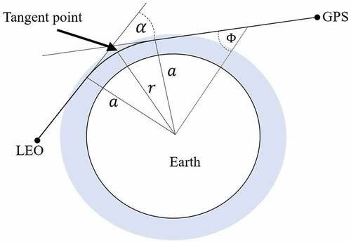The technique also requires the assumption of a spherically symmetric atmosphere (the refractive index only has radial variation) and thus the horizontal resolution is limited to the horizontal drift of the tangent point and is on the order of $\sim 100$ km (Kuo et al. 2000; Bizzarri et al. 2004). The geometry of the radio-occultation technique is shown in Figure 1. Radio-occultation sounding has been investigated using airborne receivers by Haase et al. (2014), however, the measuring capability could only be extended to the first 2 km above the surface and still suffered from poor horizontal resolution.

Figure 1. Instantaneous occultation geometry for a GPS and a low earth orbit (LEO) satellite. The impact parameter, $a$, and the bending angle of the ray, $\alpha$, are determined from the velocity and position measurements of the satellites, as well as the Doppler shift of the radio signal. The zenith angle of the ray (angle between the ray vector and the Earth radius vector) is given by $\mathrm{\Phi }$.

Ground-based measurements of GNSS signals measure the refractivity-induced delay of the signals and are widely used to estimate the vertically integrated total delay. The atmosphere is discretised into cells called voxels, each with a constant refractive index. The contribution of each voxel to the total delay of the GNSS signal forms a (sparse) system of linear equations, which can be inverted using techniques such as singular value decomposition to determine the refractive index profile (Menke 2018). Ray paths with elevations under $\sim 10$° are neglected due to significant bending, and thus the spatial resolution of the humidity field at lower altitudes is rather limited (de Haan 2008). The total delay of many signals is currently assimilated into NWP models, rather than the individual delay measurements on explicit receiver-satellite paths. Therefore the number of GPS satellites from which delay measurements can be made limits the resolution of the retrieval. In particular, the horizontal resolution is restricted by the distance between GPS receivers (Zhao, Zhang, and Yao 2019). The Met Office has been assimilating delay observations derived from ground-based GPS receivers into NWP models since 2007, and currently operates 120 receivers (Watson and Coleman 2010). However, despite the demonstrated usefulness of assimilating delay observations into NWP models, problems arise due to the low density of observations in the lower atmosphere (especially near the horizon), as well as biases in the data (Bennitt and Jupp 2012).

Fabry et al. (1997) showed that small changes in the apparent radar range of targets in the radar field of view can be used to calculate increments in path-averaged refractivity. The changes in refractivity along the length of the signal path result in a change of phase in the received signal, which can be used as a proxy for the travel time. Considering all azimuths around the radar tower allows a field of refractivity increments to be constructed. However, the technique is highly dependent on a suitable distribution of targets from which reflected signals can be measured. Swaying vegetation and sharp refractivity gradients can also significantly decrease the quality of retrievals (Weckwerth et al. 2005). The incremental refractivity data is also difficult to assimilate in comparison to absolute refractivity values.

Interest in novel humidity measurement techniques that can attain the desired resolution has grown significantly in recent years, despite previous beliefs that humidity observations had minimal impact on forecast skill beyond 1–2 days. It was originally assumed that the humidity field itself was dependent on the temperature and pressure fields, meaning that if a model integration starts with an incorrect humidity field, the field will evolve to become consistent with the well-known temperature and pressure fields (Bengtsson and Hodges 2005). Humidity observations were thought to only have a significant impact on short-range forecasts. For example, the inclusion of moisture profile sets from the Lidar Atmospheric Sensing Experiment (LASE) developed by NASA resulted in a reduction in the hurricane track and intensity errors of 100 km and $20-25\mathrm{\%}$respectively for 3-day forecasts, as shown by Kamineni et al. (2003). However, more recently it has been shown that humidity observations have a significant impact on forecasting skill over longer timescales than previously thought. Geer et al. (2017) demonstrated that the inclusion of all-sky microwave humidity measurements in the ECMWF operational system resulted in a statistically significant improvement in forecast skill out to day 5 or 6. These findings indicate that good knowledge of the spatiotemporal distribution of water vapour in the lower atmosphere has a significant impact on improving forecast skill by improving the initialization of NWP models. There is currently a significant absence of high-density humidity measurements in the lowest few kilometres of the atmosphere. Measuring humidity using the refraction of aircraft radio broadcasts has clear advantages over radio-occultation and ground-based GNSS receiver methods, since measurements are contained entirely within the troposphere, with the most information-dense measurements localized within the first few kilometres of the surface.

Other options for further enhancement of the volume of humidity data seem to be both limited and/or expensive. An in-situ sensor designed for installation on commercial aircraft has been under trial for several years in Europe, but widespread adoption seems to be some way off. New Raman and DIAL lidars are under development by commercial manufacturers and could provide detailed vertical profiles in the future. However, the number of units that could conceivably be procured for operational use would almost certainly result in a sparse network that was insufficient to meet the requirement. There is then a requirement for high-volume/low-cost measurements of atmospheric humidity or refractivity with which to initialize high-resolution operational weather forecast models. Remote sensing of the Earth’s atmosphere has historically been carried out using bespoke instruments and infrastructure: e.g. radar and satellite networks. But there are emerging possibilities offered by the opportunistic use of existing infrastructure and low-cost, mass-market technology. A largely opportunistic technique is described here for acquiring refractivity information that is complementary to the existing refractivity methods.

2. The innovation

It is proposed to use simple two-element interferometers sited on hilltops to measure the angle-of-arrival (AoA) of radio transmissions that have undergone measurable bending by the atmosphere. If the AoA is measured, and the point of origin of the signals is known accurately, then the bending angle can be computed and information extracted concerning the refractivity structure of the atmosphere. The radio transmissions are the 1090 MHz Automatic Dependent Surveillance-Broadcast (ADS-B) transmissions which all commercial aircraft are mandated to broadcast for air traffic and anti-collision purposes. The signals will undergo measurable bending a) as aircraft ’rise’ or ’set’ over the radio horizon (which will normally occur at ranges of 400 km+ for aircraft at cruise altitude) or b) at shorter ranges for aircraft taking off or landing. A preliminary sensitivity study suggests that the aircraft position is known sufficiently accurately for the bending angle calculation, but in order to detect meteorologically significant changes in refractivity, AoAs of $<\sim 2$° above the horizon will need to be measured with an accuracy of $0.01$° or better. This accuracy shall be referred to throughout this paper as the target resolution. This in turn will require an interferometer with an unobstructed view of the horizon and a (vertical) baseline of 10 m. It is proposed to make use of weather radar towers to mount the interferometer elements, thereby avoiding the need for a bespoke frame to provide a baseline with the necessary structural stability and rigidity. The interferometers can make use of Software-Defined Radio (SDR) modules, which can be easily programmed to provide the required functionality. ADS-B broadcasts conveniently contain the essential information on the aircraft location and open-source ADS-B decoders are readily available. The technique is then self-contained, requiring no external inputs or consents, and a minimum of additional hardware or infrastructure. It could be implemented anywhere in the world with a usable density of civil air traffic. For example, ${10}^3$ aircraft enter or leave UK airspace each day, with similar numbers landing and taking off from UK airports. ADS-B messages are broadcast roughly twice per second, and could be received by any hill-top interferometer that has line of sight. There is then the potential to acquire ${10}^5$-${10}^6$ bending angle measurements per day for assimilation into NWP models. The closest published technique found in the literature is due to Vowles (2007), who used a ground-based interferometer to measure the AoA of signals on terrestrial point-to-point communications links. The observed variations in AoA were related to changes in the refractivity structure and the synoptic meteorology. The use of an interferometer to measure the AoA of ADS-B broadcasts has also been proposed by Faragher, MacDoran, and Mathews (2014) to prevent spoofing attacks.

2.1. ADS-B

By June 2023, commercial aircraft above 5700 kg are mandated to broadcast digitally-encoded 3D position, along with in-situ measurements of pressure and temperature (in the form of Mach number) via the Automatic Dependent Surveillance-Broadcast (ADS-B) system, see e.g. https://en.wikipedia.org/wiki/Automatic_dependent_surveillance_-_broadcast. The broadcasts use a frequency of 1090 MHz, a frequency that is immune from significant atmospheric attenuation or diffraction and is easily received right out to the radio horizon. ADS-B broadcasts are very short – only 112 microseconds – but the signal strength is such that Software-Defined Radio (SDR) receivers and omni-directional antennas, designed mainly for the amateur market, can be employed to acquire and decode the transmissions. The digital encoding of data is using pulse-position-modulation (PPM) – each microsecond of the broadcast is ‘ON’ (high-amplitude) for either the first or second half-microsecond and ‘OFF’ (zero amplitude) for the other half-microsecond – encoding a binary 1 or 0 respectively. A 112 microsecond broadcast therefore encodes 112 bits of data, specifying the data content; the data itself; flags to denote the accuracy of the reported data; and a parity-check to validate the successful decode. Decoding software developed by amateur plane enthusiasts is freely available for download.

The use of decoded ADS-B messages to determine atmospheric conditions is not unique to this investigation and has been previously shown to be a feasible method of atmospheric sounding in several studies. For example, the air pressure and position readings from decoded aircraft ADS-B messages have been shown to be sufficiently accurate enough to determine mean layer air temperatures, as shown by Stone and Kitchen (2015). The discrepancy between the GNSS altitude and the true altitude was on the order of 10 m, and thus the accuracy was deemed to be below the reporting resolution. In this investigation the distance to the radio sources will be on the order of ${10}^4$-${10}^5$ m, hence the reported altitude readings are thought to be accurate enough for precise reported AoA measurements to be made. However, what is less certain is the impact of latency on the AoA measurement accuracy. For example, the Radio Technical Commission for Aeronautics (RTCA 2011) recommends that the uncompensated latency (time difference between the GPS update and the broadcast) should be limited to less than 200 milliseconds, meaning that an aircraft travelling parallel to the line of sight may be tens of metres further along its flight path than it reports. Verbraak et al. (2017) found that the cross-track accuracy for the position of the aircraft was 51.83 m for approximately 95$\mathrm{\%}$ of the analysed aircraft. This error is not a maximum, but represents the largest error for $\sim 95\mathrm{\%}$ of aircraft analysed. ADS-B is a subset of the wider mode-selective enhanced surveillance (Mode-S EHS) used by aircraft and air traffic management (ATM) for the communication of an aircraft’s current situation (position, movement, intention, etc.). The Met Office currently operates five Mode-S receivers, four of which are collocated with operational weather radars. Mode-S EHS/ADS-B data can be used to derive both wind and temperature information at the aircraft’s location, as shown by Stone and Pearce (2016). The Dutch national weather service KNMI has also deployed a network of ADS-B receivers to acquire upper air wind and temperature data. The local ADS-B receiver at De Bilt can receive around 7000 broadcasts every hour, demonstrating the volume of observations which can be acquired every day (de Haan, de Haij, and Sondij 2013). The assimilation of ADS-B derived wind data has had a demonstrated positive impact on NWP model performance. The present proposal can be viewed as an extension of such facilities to also perform interferometry. The extension requires two slightly more advanced (but still relatively low-cost) SDRs with an accurate time and frequency reference. The two receivers are separated vertically in space and act as a two-element interferometer, the operation of which is described below.

2.2. ADS-B interferometry

The AoA of the aircraft broadcasts is deduced from the phase-delay induced between the two receiving antennas. Combined with the knowledge of the aircraft’s location, the angle of refraction of the signal between emission and observation points can be calculated. Consider a two-element interferometer, with a vector separation $B$ between antenna 1 and antenna 2. An electromagnetic signal will arrive at one antenna before the other, with the geometrical time delay given by:

(1) ${\tau }_g=\frac{B\cdot \stackrel{\mathit{ˆ}}{s}}{c},$(1)

where $\stackrel{\mathit{ˆ}}{s}$ is a unit vector in the direction of the source from the antennas (assuming plane-parallel wavefronts – i.e. source distances large compared with $B$, which is valid for an aircraft at 10–100 km distance from an interferometer spacing of $\sim 10$ m). Figure 2 depicts the geometry, for reference. While ${\tau }_g$ is normally far too short (of order picoseconds) to be measured by time-of-arrival measurements, the accumulated phase difference $\mathrm{\Omega }=2\pi \nu {\tau }_g$ is measurable ($\nu$ = signal frequency in Hz). Writing $\nu /c$ as the reciprocal of the signal wavelength ($1/\lambda$), the phase delay is then:

(2) $\mathrm{\Omega }=2\pi \frac{B\cdot \stackrel{\mathit{ˆ}}{s}}{\lambda }=2\pi \frac{B\mathrm{c}\mathrm{o}\mathrm{s}\left(z\right)}{\lambda }=2\pi \frac{B\mathrm{s}\mathrm{i}\mathrm{n}\left(\eta \right)}{\lambda },$(2)

Figure 2. Schematic two-element interferometer deployment, here depicted with the vertical baseline separation.

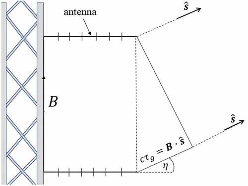
where, for a vertical baseline deployment, $z$ is the source’s (apparent) zenith angle and $\eta$ is the source’s (apparent) elevation angle above the horizon.

A software defined receiver samples complex voltage, with the Real and Imaginary components together (effectively) encoding amplitude and phase of the received voltage difference across the antenna. A signal $V_2(t)=V(t)\mathrm{e}\mathrm{x}\mathrm{p}(2\pi i\nu t)$ received at antenna 2 is simultaneous with a signal $V_1(t)=V(t)\mathrm{e}\mathrm{x}\mathrm{p}(2\pi i\nu (t-{\tau }_g))$ at antenna 1. The correlator (conjugate) product of the two signals is calculated in software via:

(3) $V_2{V}_1^{\ast }=V^2\mathrm{e}\mathrm{x}\mathrm{p}\left(2\pi i\nu {\tau }_g\right)=V^2\mathrm{e}\mathrm{x}\mathrm{p}\left(2\pi i\frac{B\cdot \stackrel{\mathit{ˆ}}{s}}{\lambda }\right)$(3)

which has amplitude $V^2$ (proportional to signal power) and phase $\mathrm{\Omega }=2\pi B\cdot \stackrel{\mathit{ˆ}}{s}/\lambda$, as noted in Equation 2(2) $\mathrm{\Omega }=2\pi \frac{B\cdot \stackrel{\mathit{ˆ}}{s}}{\lambda }=2\pi \frac{B\mathrm{c}\mathrm{o}\mathrm{s}\left(z\right)}{\lambda }=2\pi \frac{B\mathrm{s}\mathrm{i}\mathrm{n}\left(\eta \right)}{\lambda },$(2) . It is possible therefore to use the correlator amplitude to decode ADS-B messages and the correlator phase to deduce AoA. Normally, for large $B/\lambda$, the phase (defined practically between [-$\pi$,+$\pi$]) corresponds to multiple possible angles-of-arrival across the sky. However, ADS-B positional information allows for the unambiguous selection of the correct phase period. High values of $B/\lambda$ are desirable, as they result in accurate angle-of-arrival measurements for a given phase uncertainty.

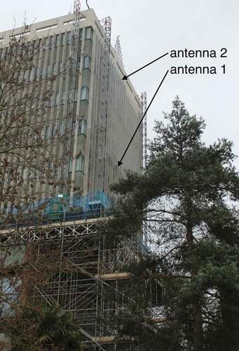
The theoretical AoA uncertainty for a vertical baseline of 10 m is very small: ${\sigma }_{\mathrm{A}\mathrm{o}\mathrm{A}}={\sigma }_{\mathrm{\Omega }}/2\pi (B/\lambda )$ where ${\sigma }_{\mathrm{\Omega }}=0.015$ is our measured phase uncertainty for a typical ADS-B broadcast (${\sigma }_{\mathrm{A}\mathrm{o}\mathrm{A}}=0.004$° for a baseline of 10 m). Achieving such accuracy would allow for the retrieval of refractivity profiles with remarkable resolution, however, the technical challenge of achieving such accuracy will be demanding. Preliminary experimental tests have been conducted at the University of Exeter. An experimental interferometer, comprising an Ettus X300 SDR equipped with a GPS-disciplined oven-controlled crystal oscillator (GPSDO/OCXO) for time and frequency referencing, accepts two equal-length feeds from monopole antennas which have been deployed on a 10 m vertical baseline as shown in Figure 3.

Figure 3. Experimental two-element interferometer deployed on the Physics Building at the University of Exeter.

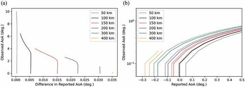
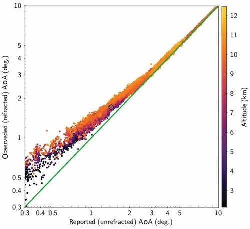
Figure 4(a) shows the measured phase accuracy using the experimental interferometer installed on the Physics Building. Figure 4(b) shows the implied AoA accuracy. The results indicate that a $0.01$° resolution should be achievable, however, there are currently residuals on the order of $\sim 0.03$°. Publicly-available ADS-B software is used for decoding the correlator amplitude, and a phase extractor has been synthesized with the ADS-B code. Figure 5 shows some preliminary measurements from the interferometer. Measured AoAs are plotted against unrefracted aircraft elevation angles derived from decoded aircraft locations. The interferometer field of view is to the south of Exeter, out over the English Channel. Each point represents a single ADS-B transmission containing a positional update, and the $\sim$ 60,000 data points plotted here were obtained over a 4-hour period. The data points from low altitudes originate from aircraft taking off and landing from the airports in the Channel Islands. The clear separation of the colours in Figure 5 shows that the signals originating from aircraft at higher altitudes tend to undergo greater refraction for a given observed AoA. This is to be expected given the lower average values of refractivity at higher altitudes, and demonstrates that there is information concerning the refractivity structure contained within the data. Whilst this is an encouraging start, it is acknowledged that much more work is required before the technique is proven to deliver useful data.

Figure 4. (a) Measured phase accuracy from experimental interferometer located at the Physics Building, University of Exeter. (b) Implied AoA accuracy from the experimental interferometer. Residuals in practice were 0.03°.

Figure 5. Interferometrically-measured observed AoA versus reported AoA deduced from decoded ADS-B data. The green line is a line of equality (not a fit).

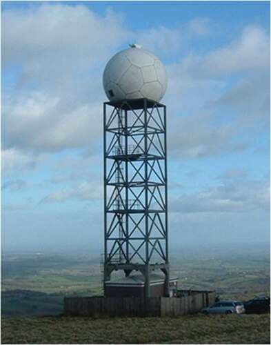
More recently, a prototype interferometer has been installed at Clee Hill radar tower in Shropshire (Figure 6), however, the AoA uncertainty is currently still greater than the target of $0.01$°. A potential source of uncertainty are multipath effects where ground reflections in the foreground interfere with the direct (least-time) signal. Work is currently being done to minimize sources of uncertainty, including the development of absorbing shields to block reflected signals before they can reach the interferometer antennas.

Figure 6. Clee Hill radar tower in Shropshire. See https://www.metoffice.gov.uk/research/news/2019/harry-otten-prize-observation-award.

2.3. Atmospheric refraction

The parts-per-million (ppm) excess of the refractive index $n$ over the unity vacuum value is encoded by the parameter $n$ according to:

(4) $n=1+\frac{N}{{10}^6}.$(4)

Empirical calibrations of $N$ account for ’dry’ and ’wet’ contributions according to:

(5) $N=\frac{aP}{T}+\frac{be}{T^2},$(5)

where $P$, $T$, $e$ are pressure, temperature, and water vapour pressure (WVP) respectively, and the empirical constants $a$ and $b$ are 77.6 K/hPa and $3.73\times {10}^5$ K²/hPa respectively (Smith and Weintraub 1953). A representative value of $N$ at ground level is $N\approx 300$ ppm, which includes a $\sim 10\mathrm{\%}$ contribution from WVP. For air at a temperature and pressure of 293.15 K ($20$°C) and 1013 hPa respectively, there is a rough equivalence that a 1$\mathrm{\%}$ change in relative humidity produces a change in refractivity of 1 ppm. The dry contribution is largely static as it depends on the overall atmospheric density structure, while the wet contribution can vary significantly over both short spatial and temporal scales (Wadge et al. 2016). Additional contributions from trace atmospheric constituents (e.g. liquid water, ice, aerosols) can be included, though these are very small compared to the main wet and dry contributions (Solheim et al. 1999). In-situ pressure and temperature can be acquired through Mode-S broadcasts, so that a measurement of refraction (constraining $N$) via interferometry can therefore yield an estimate of the water vapour pressure $e$. Pressure and temperature measurements throughout the extent of the lower atmosphere can be made via Mode-S broadcasts from aircraft at various altitudes (e.g. aircraft landing/taking off at airports). This would allow for the decoupling of the wet and dry refractivity contributions and an estimate of the humidity distribution in the lower atmosphere.

3. Ray-tracing

The propagation of radio waves in the troposphere can be modelled using ray-tracing in a time-reversed frame from the observer to the source. This time-reversed frame allows the known parameters at the observer’s position (refractive index and observed AoA) to be used as the boundary conditions. In the ray-tracing framework, the influence of model and realistic atmospheres on the ray path can be determined which allows for the prediction of the observed AoA measurements based on the atmospheric conditions and the position of the ray source. The spherically symmetric and spherically asymmetric atmosphere models are investigated here, the former utilizing Snell’s law whereas the latter utilizes the scalar wave equation.

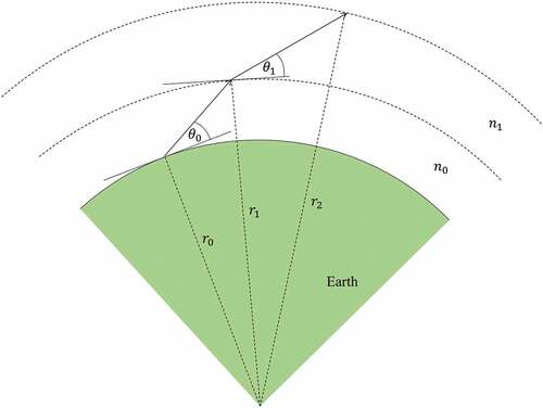
The atmosphere in most cases can be reasonably assumed to be spherically symmetric (that is, the refractive index depends only on the radial distance from the centre of the Earth). With this assumption, the path of a radio ray can be modelled using a generalization of Snell’s law to a radially directed refractive index gradient:

(6) $n_i{r}_i\mathrm{c}\mathrm{o}\mathrm{s}({\theta }_i)=n_{i+1}{r}_{i+1}\mathrm{c}\mathrm{o}\mathrm{s}({\theta }_{i+1})=\mathrm{C},$(6)

where $n$ is the refractive index, $r$ is the radius of the ray (distance to the centre of the Earth), $\theta$ is the elevation of the ray above the local horizon, $i\in \mathbb{Z}$ is the index of each iteration along the ray path and C is a constant. Figure 7 shows the geometry of the ray-tracing system. The quantity $nr\mathrm{c}\mathrm{o}\mathrm{s}(\theta )$ is constant along every point on the ray path, and thus in the time-reversed frame the entire path can be traced with knowledge of the surface refractive index and the observed AoA (${\theta }_0$).

Figure 7. Two-dimensional geometry of the refraction of a radio ray through the atmosphere. The radius (distance to the centre of the Earth) and local elevation angle of the ray at every step are given by $r_i$ and ${\theta }_i$ respectively (where $i$ is the iteration index). The refractive index of each layer of the atmosphere is given by $n_i$. The refractive index is one-dimensional and varies only with height (radially). The initial elevation angle of the ray ${\theta }_0$ is equivalent to the observed AoA.

In most ray-tracing models, the atmospheric refractivity is assumed to be spherically symmetric (i.e. no horizontal variations). However, to simulate the path of radio rays through a realistic atmosphere, both the horizontal and vertical variations in refractivity should be considered. The ray-tracing model used here was derived by Kerr (1987) and involves solving the scalar wave equation:

(7) ${\mathrm{\nabla }}^2\mathrm{\Psi }+k^2{n}^2\mathrm{\Psi }=0,$(7)

seeking solutions of the form:

(8) $\mathrm{\Psi }=Q\mathrm{e}\mathrm{x}\mathrm{p}(-ikS),$(8)

where $S$ and $Q$ are real functions of position. Substituting (8) into Equation 7(7) ${\mathrm{\nabla }}^2\mathrm{\Psi }+k^2{n}^2\mathrm{\Psi }=0,$(7) , extracting the real part and assuming $k$ is large (i.e. considering only high frequencies), Equation 7(7) ${\mathrm{\nabla }}^2\mathrm{\Psi }+k^2{n}^2\mathrm{\Psi }=0,$(7) can be reduced to the eikonal equation, given by:

(9) $(\mathrm{\nabla }S{)}^2=n^2,$(9)

where $S$ is known as the eikonal and $n$ is the refractive index. Surfaces of constant $S$ are the wavefronts of the solution of the wave equation. The curvature at any point along the ray path can be calculated in terms of the relative angle $\gamma$ between the direction of the ray and the direction of the gradient of refractive index $\mathrm{\nabla }n$ by:

(10) $K=\left|\frac{\mathrm{d}t}{\mathrm{d}s}\right|=\frac{\left|\mathrm{\nabla }n\right|\mathrm{s}\mathrm{i}\mathrm{n}\left(\gamma \right)}{n},$(10)

where $K$ is the curvature of the ray, $t$ is the unit vector in the direction of the ray path at each point and $\mathrm{d}s=\mathrm{d}S/n$ is the infinitesimal arc length of the ray. In order to trace rays through the atmosphere, the relative curvature of the ray with respect to the surface of Earth must be known. The relative curvature is given by:

(11) $K_r=\frac{\mathrm{d}\theta }{\mathrm{d}s}=\frac{\mathrm{d}\varphi }{\mathrm{d}s}-\frac{\mathrm{d}t}{\mathrm{d}s},$(11)

where $\theta$ is the local ray elevation angle and $\varphi$ is the angle subtended by the ray at the centre of the Earth. The relative curvature can be written in terms of the curvature of the ray $K$ in (10) by:

(12) $K_r=\frac{\mathrm{c}\mathrm{o}\mathrm{s}(\theta )}{r+h}-K,$(12)

where $r+h$ is the radius of the ray at any point along the ray path.

From Figure 8 it can be seen that:

(13) $\mathrm{s}\mathrm{i}\mathrm{n}(\gamma )=\mathrm{c}\mathrm{o}\mathrm{s}(\theta -\psi )=\mathrm{c}\mathrm{o}\mathrm{s}(\theta )\mathrm{c}\mathrm{o}\mathrm{s}(\psi )+\mathrm{s}\mathrm{i}\mathrm{n}(\theta )\mathrm{s}\mathrm{i}\mathrm{n}(\psi ),$(13)

Figure 8. Geometry of the ray path through an atmosphere with spherical asymmetry (geometry used by Martin and Wright 1963).

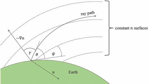
with:

(14) $\begin{array}{rl}& \mathrm{c}\mathrm{o}\mathrm{s}(\psi )=-\frac{1}{\left|\mathrm{\nabla }n\right|}\frac{\mathrm{\partial }n}{\mathrm{\partial }z}\\ & \mathrm{s}\mathrm{i}\mathrm{n}(\psi )=\frac{1}{\left|\mathrm{\nabla }n\right|}\frac{\mathrm{\partial }n}{\mathrm{\partial }x},\end{array}$(14)

where $\theta$ is the local ray elevation angle and $\psi$ is the angle of elevation of the constant $n$ surface. This allows Equation 10(10) $K=\left|\frac{\mathrm{d}t}{\mathrm{d}s}\right|=\frac{\left|\mathrm{\nabla }n\right|\mathrm{s}\mathrm{i}\mathrm{n}\left(\gamma \right)}{n},$(10) to be re-expressed as:

(15) $K=\frac{{10}^{-6}}{n}\left(-\mathrm{c}\mathrm{o}\mathrm{s}(\theta )\frac{\mathrm{\partial }N}{\mathrm{\partial }z}+\mathrm{s}\mathrm{i}\mathrm{n}(\theta )\frac{\mathrm{\partial }N}{\mathrm{\partial }x}\right),$(15)

where the relationship $n=1+N/{10}^6$ has been employed. With knowledge of the curvature of the ray at any point (as well as the relative curvature of the ray with respect to the surface of the Earth), the ray path through an inhomogeneous atmosphere can be traced. In practice the arc length increment $\mathrm{d}s\to \mathrm{\Delta }s=0.3$ km is used. Ray-tracing through two-dimensional refractivity fields will be required when reconstructing humidity fields with horizontal variations. The impact of one- and two-dimensional refractivity fields on the refraction of ADS-B broadcasts will be outlined below.

4. Sensitivity tests

4.1. Tests using idealised atmospheres

In contrast to temperature and pressure, the variation in relative humidity (RH) with altitude is not easily modelled using a simple functional form. The impact that a constant RH vertical profile had on the observed refraction was investigated by determining the saturation pressure of water vapour. The saturation pressure, $e_s$, is the maximum vapour pressure that can occur at a given temperature and pressure before condensation occurs. The saturation pressure of water vapour can be calculated using the Arden Buck equations (Buck 1996):

(16) $e_s(T)=\left\{\begin{array}{cc}6.1121\mathrm{e}\mathrm{x}\mathrm{p}[f_1(T)],& T\ge 0^{\circ }\mathrm{C}\\ 6.1115\mathrm{e}\mathrm{x}\mathrm{p}[f_2(T)],& T<0^{\circ }\mathrm{C},\end{array}\right.$(16)

where $f_1(T)$ and $f_2(T)$ are given by:

(17) $f_1(T)=\left(18.678-\frac{T}{234.5}\right)\left(\frac{T}{T+257.14}\right),$(17)

and

(18) $f_2(T)=\left(23.036-\frac{T}{333.7}\right)\left(\frac{T}{T+279.82}\right),$(18)

respectively. The maximum possible partial pressure of water vapour increases exponentially with increasing temperature, and thus warmer humid air has a greater impact on refraction than colder humid air. The impact of a constant RH profile on the refraction of radio waves can be determined by calculating the ratio of the vapour pressure of water vapour with the saturation vapour pressure.

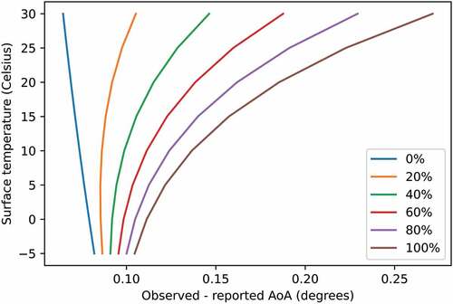
Figure 9 demonstrates how the difference between the observed and reported AoA increases dramatically with increasing air temperature and RH for a ray source at a distance of 100 km from the observer with an observed AoA of $1.0$°. The surface air pressure and lapse rate were held constant at the standard International Civil Aviation Organisation (ICAO) atmosphere values of 1013.25 hPa and 6.5 K/km respectively. The RH was uniform throughout the modelled atmosphere. At $0\mathrm{\%}$ RH ($e=0$ hPa), the observed – reported AoA decreases with increasing temperature due to the zero contribution of the wet refractivity term to the total refractivity. The remaining dry refractivity term is inversely proportional to temperature, and thus refraction decreases with increasing temperature (keeping the pressure profile the same). At higher RH and air temperatures the observed – reported AoA increases exponentially. At $100\mathrm{\%}$ RH (corresponding to the air being at its dew point temperature) and high temperatures the observed – reported AoA becomes very large (exceeding 25 times the target resolution of 0.01°). It is therefore expected that ADS-B interferometry will be most sensitive to atmospheric refractivity structures during the warmer and more humid summer months.

Figure 9. The dependence of the observed – reported AoA on both the RH and surface air temperature for a ray source 100 km away with an observed AoA of 1.0°.

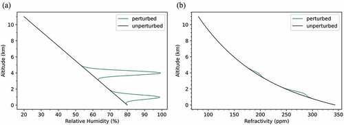
Regions of the atmosphere can become saturated with water vapour (where RH is close to or at 100$\mathrm{\%}$) and form cloud layers. An initial idealized atmosphere was constructed using an RH vertical profile that decreased linearly with altitude from a maximum of 80$\mathrm{\%}$ at the surface to a minimum of 20$\mathrm{\%}$ at the tropopause ($\sim 11$ km). Regions of saturated air (RH = 100$\mathrm{\%}$) were added as perturbations to the linear RH vertical profile to simulate cloud layers. Figures 10(a) and Figure 10(b) show that the perturbation in the vertical RH profile had a corresponding impact on the vertical refractivity profile. The temperature and pressure at the surface were fixed at $T_0=288.15$ K ($15$°C) and $p_0=1013.25$ hPa respectively. The modelled temperature varied linearly as $T(h)=T_0-6.5h$ and the modelled pressure varied as $p(h)=p_0[1-(6.5h/T_0){]}^{5.2561}$ with height $h$ (in km) (from the ICAO standard atmosphere). Rays were traced through the perturbed and unperturbed refractivity fields and the reported AoA was calculated for both.

Figure 10. (a) Background vertical RH profile (black) with two perturbations of nearly saturated air centred at 1.5 km and 4.0 km (green). The perturbations simulate cloud layers centred at an altitude of 1.5 km and 4.0 km. (b) Background vertical refractivity profile (black) with two perturbations of nearly saturated air centred at 1.5 km and 4.0 km (green). The perturbations simulate cloud layers centred at an altitude of 1.5 km and 4.0 km.

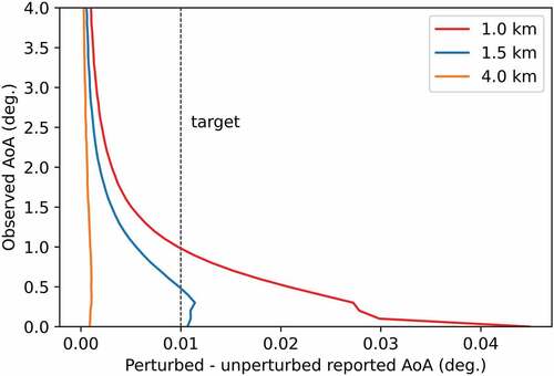
The difference in the reported AoA for the perturbed and unperturbed RH vertical profiles in Figure 11 was largest for observed AoAs close to the horizon ($<\sim 1.5$°) with simulated cloud layers 1.0 km above the surface. The ability to detect RH perturbations rapidly deteriorated as the altitude of the perturbation increased due to the corresponding decrease in vapour pressure. For a cloud layer centred at an altitude of 4.0 km, the impact of the RH perturbation on the vertical refractivity profile was smaller than for a cloud layer centred at an altitude of 1.5 km. This was due to the smaller refractivity gradient in the region of the cloud. The difference in the perturbed and unperturbed reported AoA did not exceed the target resolution of $0.01$° for a cloud layer centred at 4.0 km.

Figure 11. Difference in the observed – reported AoA between the perturbed and unperturbed vertical RH gradients for observed AoAs ranging from 0.0° to 4.0°.

For these simulations using a 1D model atmosphere, Snell’s law was used to calculate the AoA measurements by assuming a spherically symmetric atmosphere. The refractivity decayed exponentially with altitude by:

(19) $N=N_0\mathrm{e}\mathrm{x}\mathrm{p}\left(\frac{-h}{H}\right),$(19)

where $N_0$ is the surface refractivity (in this case equal to 300 ppm), $h$ is height and $H$ is the scale height of the atmosphere (in km respectively), given by:

(20) $H=\frac{RT}{Mg},$(20)

where $R$ is the universal gas constant ($\approx 8.314$ J mol⁻¹ K⁻¹), $T$ is the air temperature (in Kelvin), $M$ is the molar mass of the atmosphere ($\approx 0.029$ kg mol⁻¹) and $g$ is the acceleration due to gravity ($g=9.81$ ms⁻²).

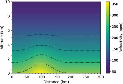
To simulate the impact of spherical asymmetry on the AoA, an arbitrary position-dependent perturbation centred at a distance of 100 km was added to the refractivity profile, described by Equation 19(19) $N=N_0\mathrm{e}\mathrm{x}\mathrm{p}\left(\frac{-h}{H}\right),$(19) . The magnitude of the refractivity perturbation was 60 ppm and was of the form:

(21) $N{ }^{\mathrm{\prime }}=\left\{\begin{array}{cc}(60-10h)\mathrm{e}\mathrm{x}\mathrm{p}\left(\frac{-{(X-100)}^2}{2000}\right),& h\le 6\mathrm{k}\mathrm{m}\\ 0,& h>6\mathrm{k}\mathrm{m}\end{array}\right.$(21)

where $X$ is the horizontal distance (in km). The perturbation magnitude was scaled to ensure $N{ }^{\mathrm{\prime }}=0$ ppm at an altitude of 6 km, preventing any abrupt change in refractivity. This was decided to create a more realistic refractivity profile, especially at higher altitudes where the refractivity is dominated by the dry atmospheric gases and is relatively stable. The resulting refractivity profile is shown in Figure 12.

Figure 12. Vertical and horizontal profile of refractivity. The refractivity has a dependence on both the vertical and horizontal position. The surface refractivity at a distance of 100 km is equal to 360 ppm. Contours of constant refractivity at 300 ppm, 250 ppm, 200 ppm and 150 ppm are indicated by the dashed lines.

To investigate the influence that the perturbation $N{ }^{\mathrm{\prime }}$ had on the AoA, the two-dimensional ray-tracing model was employed. In a time-reversed frame, 100 rays were traced through the perturbed and unperturbed atmospheres and the respective reported AoAs were recorded. The maximum ray altitude was capped at 12 km. The difference between the perturbed and unperturbed reported AoA was calculated for each ray. Figure 13(a) shows the difference between the perturbed and unperturbed reported AoA as a function of observed AoA. Figure 13(b) shows the perturbed (dashed) and unperturbed (solid) reported AoA values as a function of observed AoA. The difference between the perturbed and unperturbed reported AoA was largest ($\sim 0.035$°) for sources 400 km away with observed AoAs $<1.0$°, but did not exceed the target resolution of $0.01$° for source ranges of 50 km and 100 km.

Figure 13. (a) The difference in the reported AoA between the unperturbed and perturbed refractivity fields as a function of observed AoA. (b) The absolute reported AoAs in the perturbed (dashed) and unperturbed (solid) refractivity fields as a function of observed AoA.

These results indicate that horizontal variations in the refractivity field would only just exceed the detectable threshold and thus in certain limited situations (e.g. frontal systems with large horizontal gradients) the spherically stratified assumption may no longer be adequate to accurately predict the observed AoA. Retrieving two- and three-dimensional refractivity fields will also of course require treatment of the horizontal component of refractivity fields.

4.2. Tests using radiosonde data

The refraction that occurs in a realistic atmosphere was determined using data from Vaisala RS41 radiosondes launched from Watnall, Nottinghamshire in July 2021. As the radiosonde ascended the atmospheric conditions were recorded at intervals of 2 seconds. Figure 14(a) shows the RH vertical profile over Watnall at 11:15 UTC (blue) and at 23:15 UTC (black) on the 27^th of July 2021. There is significant variation in the RH over the course of 12 hours, particularly in the first $\sim 3$ km above the surface where a region of relatively low RH is situated in the 11:15 UTC data. Only the first $\sim 11$ km (up to approximately the tropopause) have been shown. Figure 14(b) shows the corresponding mixing ratio vertical profile over Watnall at 11:15 UTC (blue) and at 23:15 UTC (black) on the 27^th of July 2021. Despite the RH being above 80$\mathrm{\%}$ even at $\sim 7$ km above the surface, the mixing ratio (mass of water vapour per unit mass of dry air) is low. Figure 15 demonstrates how the mixing ratio of water vapour contributes little to the total refractivity at high altitudes. There is significant variation in the RH vertical profile over the course of 12 hours between readings, particularly in the first few kilometres above the surface.

Figure 14. (a) RH vertical profile determined using radiosonde readings from the 27${ }^{\mathrm{t}\mathrm{h}}$ of July 2021 at 11:15 UTC (blue) and at 23:15 UTC (black). (b) Mixing ratio vertical profile determined using radiosonde readings from the 27${ }^{\mathrm{t}\mathrm{h}}$ of July 2021 at 11:15 UTC (blue) and at 23:15 UTC (black).

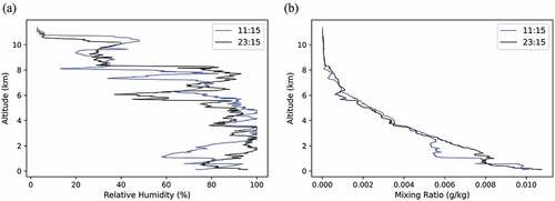
Figure 15. Vertical profile of dry refractivity (dashed lines) and wet plus dry refractivity (solid lines) over Watnall determined using the data obtained by radiosondes launched at 11:15 UTC (blue) and 23:15 (black) UTC on the 27${ }^{\mathrm{t}\mathrm{h}}$ of July 2021.

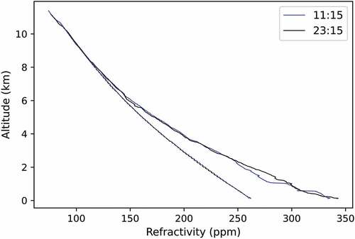
Figure 15 shows the dry refractivity vertical profile and the total (wet plus dry) refractivity profile determined using radiosonde readings. The dry refractivity decreases almost exponentially with altitude and shows very little variation over the 12 hour period. The wet refractivity contributes significantly more variation, with the most significant perturbations at an altitude of $\sim 2$ km. It can therefore be deduced in this example that any variation in the refraction of aircraft radio broadcasts over the 12 hour period will be predominantly due to variations in the wet refractivity.

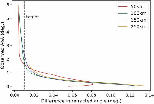
Near the surface, where solar heating and evaporation of water occur, is where significant variations in refractivity are most likely. It can be seen in Figure 15 that the wet refractivity contribution to the total refractivity is essentially negligible above an altitude of $\sim 7$-$8$ km, suggesting that RH vertical profile retrievals above this will be practically impossible. Figure 16 shows the difference in the refracted angle (observed – reported AoA) for rays traced in the 11:15 UTC and 23:15 UTC RH vertical profiles. Variations in the refracted angle exceeded the target resolution below $\sim 2$°, and were largest for more distant sources.

Figure 16. Difference in refracted angle (observed – reported AoA) for rays traced in atmospheres modelled using radiosonde data for 11:15 UTC and 23:15 UTC on the 27${ }^{\mathrm{t}\mathrm{h}}$ of July 2021. More distant sources with low observed AoAs undergo the greatest refraction. For observed AoAs greater than 2°, the difference in the refracted angle between the 11:15 UTC and 23:15 UTC RH vertical profiles does not exceed the target resolution.

4.3. Sources of uncertainty in reported AoA

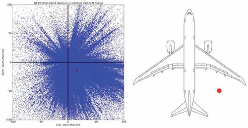
The accuracy of the reported AoA is dependent on the accuracy of the reported position of the aircraft. The reported horizontal position of the aircraft is dependent on both the latency and the cross-track offset. The latency is the time interval between the position determination inside the aircraft and the signal registration by the receiver. The aircraft can travel on the order of 40 m during the few hundred milliseconds between receiving position information from GNSS satellites and transmitting the data to the receiver. The cross-track offset is determined by comparing the ADS-B reported horizontal position with that determined by radar. The cross-track accuracy for the position of the aircraft was found to be 51.83 m for approximately 95$\mathrm{\%}$ of the aircraft analysed by Verbraak et al. (2017). The distribution is shown in Figure 17. The reported AoA must be known accurately since the difference between the observed and reported AoA is generally $<0.5$°.

Figure 17. Left: Plot showing the directional offset of all flights departing and arriving at Schiphol airport on the 11${ }^{\mathrm{t}\mathrm{h}}$ of January 2016. Right: The red dot indicates the average offset compared to the centre point of a Boeing 787 Dreamliner (from Verbraak et al. 2017).

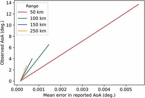
The maximum horizontal position error due to uncompensated latency was assumed to be 40 m in the direction parallel to the line of sight to the reporting aircraft. The maximum vertical and horizontal positions of the modelled aircraft were 12 km and 250 km respectively. The modelled aircraft were in level flight travelling at a ground speed of 200 ms⁻¹. Figure 18 shows the resulting error in the observed AoA measurement. The error in the observed AoA increased with the observed AoA and decreased with increasing range to the source. This is expected since horizontal position errors on the order of $\sim 10$ m do not significantly change the observed elevation angle of aircraft at larger distances. For nearby sources with high observed AoAs, the horizontal position error has a significantly larger impact on the measured AoA accuracy. However, for the range of sources investigated here, the mean error did not exceed the target resolution of $0.01$°. The latency will result in the observed position having a vertical component if the aircraft is either descending or ascending. For example, an aircraft descending at 15 ms⁻¹ with a horizontal velocity of 100 ms⁻¹ directed along the line of sight will have a vertical position error of 3 m (assuming a latency of 0.2 seconds).

Figure 18. Error in the observed AoA assuming a latency in the ADS-B broadcasts of 0.2 seconds and an aircraft ground speed of 200 ms${ }^{-1}$ directly parallel to the line of sight. The uncompensated latency resulted in a position error of 40 m either closer to or further from the observer. Large observed AoAs resulted in larger errors in the measured ray bending, especially for nearby sources.

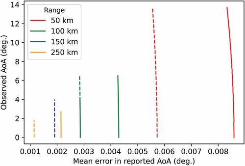
The uncertainty in the vertical position of the aircraft had a larger contribution to the observed AoA error than the horizontal position uncertainty. Figure 19 shows the mean error in the observed AoA assuming a vertical position error of 10 m (dashed lines) and 15 m (solid lines) for aircraft ranging in distance from 50 km to 250 km. For a vertical position error of 15 m, the uncertainty in the reported AoA increased considerably with decreasing distance to the source. However, the uncertainty in the reported AoA did not exceed $0.01$° for any aircraft with a vertical position uncertainty of either 10 m or 15 m. The mean error in the observed AoA was highly dependent on the distance to the aircraft and did not strongly depend on the observed AoA.

Figure 19. Error in the reported AoA of broadcasts for aircraft situated at distances between 50 km and 250 km, assuming an error in the vertical position of the aircraft of 10 m (dashed) and 15 m (solid). The mean error in the reported AoA increases substantially as the distance to the aircraft decreases, but did not strongly depend on the observed AoA.

These results suggest that refraction measurements using distant aircraft with low observed AoAs are the least susceptible to errors associated with uncertainties in the horizontal and vertical positions of the aircraft. However, due to the sheer abundance of broadcasts available (each aircraft broadcasts its position multiple times per second), it may be possible to filter the measurements and reject broadcasts from aircraft whose positional uncertainties exceed a certain threshold. This could potentially be accomplished by comparing the position data of multiple broadcasts. In trial data gathered by Hayward et al. (2015), it was found that the probability of three or more ADS-B broadcasts with horizontal position errors $>300$ m was $0.0004\mathrm{\%}$. The use of the Navigational Integrity Category (NIC) recorded in the ADS-B message could also be used to assess the quality of the position estimate. The NIC is a value that represents the integrity bound of the error in the position estimate recorded in the ADS-B message (Liu, Lo, and Walter 2020). It ranges from 0 (potentially complete loss of GNSS signal with a position error integrity containment radius greater than 37.04 km) to 11 (a position error integrity containment radius of less than 7.5 m), and could be used to determine whether or not a broadcast is accepted. The vertical position uncertainty has the largest contribution to the error in the observed AoA. The discrepancy between the reported GNSS altitude and the true altitude of the aircraft is on the order of 10 m and is relatively consistent over time periods of less than 2 hours (Stone and Kitchen 2015; ICAO 2013). Thus it is expected that the majority of the observed AoA measurements will have an error not exceeding the target resolution of 0.01°. The effect of latency could introduce an extra contribution to the vertical position uncertainty for aircraft either ascending or descending, and thus the vertical and horizontal position uncertainties could be correlated as the aircraft changes in altitude. For aircraft cruising at a constant altitude, the error contributed due to the horizontal uncertainty in the position of the aircraft is not expected to contribute greatly to the error in the observed AoA. Simulated studies show that the expected uncertainty in the position of the aircraft would still allow for precise AoA measurements and an accurate RH vertical profile retrieval, particularly for more distant aircraft.

5. Extraction of refractivity structure

5.1. Inversion method

The goal is to determine the atmospheric refractivity field that causes the observed refracted angles, which is an inverse problem. The analogous radio-occultation technique requires the radio signal to pass through a point of closest approach (where the cozenith angle is $0$°). Unfortunately, the positions of both the broadcasting aircraft and ADS-B interferometer in our proposed method means that the vast majority of received broadcasts do not have a point of closest approach, and thus the inversion techniques used in radio-occultation cannot be applied to this technique. We can frame the inverse problem as trying to minimize the difference between the observed and modelled AoA data. We can define a cost function $J$ describing the misfit between the modelled and observed data as:

(22) $J=\frac{1}{N_b}\sum _{i=0}^{N_b}({\phi }_i-O_i{)}^2,$(22)

where $\phi$ is the modelled reported AoA, $O$ is the reported AoA inferred from aircraft position data, $N_b$ is the number of broadcasts and $i\in \mathbb{Z}$ is an index indicating the $i^{\mathrm{t}\mathrm{h}}$ broadcast. The cost function describes the mean squared error (MSE) between the model and observation which we seek to minimize by choosing the optimum refractivity field.

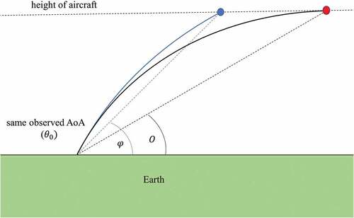
Figure 20 shows the geometry of a single ray system for which we are trying to optimize. In the following simulated experiments, we attempt to optimize a one-dimensional refractivity field (i.e. the refractivity depends only on height) by ray-tracing using the generalized spherical Snell’s law, described in Section 3. We seek to choose a refractivity field such that the misfit between the reported AoA of the modelled ray end point (blue) and the true reported AoA of the aircraft (red) is minimized. Using Figure 20 as an example, we can see that choosing a steeper refractivity gradient would result in the modelled ray being refracted more and hence decrease the difference between the modelled reported AoA, $\phi$, and the reported AoA inferred from the aircraft position data, $O$.

Figure 20. Geometry of the system to be optimized. The initial modelled ray (blue line) is traced from the position of the observer to the height of the aircraft, using the interferometrically-derived observed AoA ${\theta }_0$ as the initial elevation angle. The true position of the aircraft is given by the red point. The cost function $J$ can then be calculated by comparing the modelled reported AoA, $\phi$, to the reported AoA derived from aircraft position data, $O$.

A single ray path will contain only limited information about the detailed refractivity structure between the observer and the aircraft. A number of ray sources at a range of different heights and distances would allow us to construct a more detailed refractivity profile. Simulated annealing techniques, using a large number of broadcasts originating from a range of different positions inside the atmosphere, can be used to find a good approximation of the refractivity structure. Simulated annealing (SA) is a probabilistic technique for determining the approximate global minimum of a given function. It is analogous to the annealing process of slowly cooling a heated metal to a minimum energy state. Local energy minima are avoided by periodically accepting worse solutions with some probability that decreases with time (allowing the SA algorithm to ’jump out’ of local minima). Since the modelled reported AoA, $\phi$, is a function of the refractivity along the ray path (the ray path is defined by the refractivity field), the global minimum of our cost function, $J$, can be obtained by finding the best estimate of the true refractivity field.

To determine the best estimate of the refractivity structure, we split the initial estimate of the refractivity profile into the dry and wet components. We fixed the dry refractivity using the pressure and temperature readings from the radiosonde data. The wet component of refractivity was modified indirectly by adjusting the RH vertical profile. The decision to modify RH rather than wet refractivity directly in the annealing process was made since we can define the range 0–100$\mathrm{\%}$ for physically plausible RH values. The wet refractivity, however, also depends on temperature, and thus the domain space is less easily known initially.

The goal here is to find the best one-dimensional RH (and hence refractivity) vertical profile which minimizes $J$:

1. Choose an initial (prior) RH profile $x=(x_1,x_2,\dots ,x_i)$ (where $x_i$ is the RH at the $i^{\mathrm{t}\mathrm{h}}$ level), and convert it into a refractivity profile (assuming pressure and temperature are known).

2. Ray trace $N_b$ rays through this prior atmosphere from the observer’s position up to the positions reported in the decoded ADS-B broadcasts, using the observed AoAs (${\theta }_0$) as the initial elevation angles of the rays.

3. Determine $\phi$ for each modelled ray and calculate $J$.

4. Perturb each RH value $x_i$ in the prior atmosphere grid: $x{{ }^{\mathrm{\prime }}}_i=x_i+\mathrm{\Delta }x$ (where $\mathrm{\Delta }x\in [0,\mathrm{\Delta }{x}_{\mathrm{m}\mathrm{a}\mathrm{x}}]$ is a random step with max step size $\mathrm{\Delta }{x}_{\mathrm{m}\mathrm{a}\mathrm{x}}$). Repeat steps 2 and 3 using the new perturbed atmosphere $x{ }^{\mathrm{\prime }}$.

5. Comparing iteration $j+1$ with iteration $j$ ($j\in \mathbb{Z}$), if $J_{j+1}<J_j$, $x{ }^{\mathrm{\prime }}$ is accepted. If $J_{j+1}>J_j$, the Metropolis criterion is used to determine the acceptance of $x{ }^{\mathrm{\prime }}$. The probability:

   (23) $p=\mathrm{e}\mathrm{x}\mathrm{p}\left(-\frac{J_{j+1}-J_j}{\beta }\right)$(23)

is computed and compared with a uniformly distributed random number $p{ }^{\mathrm{\prime }}$ between 0 and 1. If $p>p{ }^{\mathrm{\prime }},x{ }^{\mathrm{\prime }}$ is accepted. Otherwise $x{ }^{\mathrm{\prime }}$ is rejected. The temperature parameter $\beta$ is decreased and steps 4 and 5 are repeated for the specified number of iterations.

The temperature parameter $\beta$ is decreased throughout the annealing process and modulates the acceptance probability. Higher initial temperatures (${\beta }_0$) at the start of the annealing process increase the probability of accepting solutions which increase the energy, allowing the SA algorithm to escape local minima. Lower temperatures later in the annealing process reduce the probability of accepting solutions which increase energy and favour solutions which minimize $J$. From the best estimate RH field the mixing ratio at each level can be calculated using (Wallace and Hobbs 2006):

(24) $w_i=(w_s{)}_i\frac{x_i}{100},$(24)

where $w_i$, $(w_s{)}_i$ and $x_i$ are the mixing ratio, saturation mixing ratio and relative humidity at the $i^{\mathrm{t}\mathrm{h}}$ level respectively. The saturation mixing ratio is given by:

(25) $w_s=0.622\frac{e_s}{p-e_s},$(25)

where $p$ and $e_s$ are the total atmospheric pressure and the saturation vapour pressure of water respectively. Prefactor: $R_d/R_v=0.622$ where $R_d$ and $R_v$ are the molar gas constants of dry air and water vapour respectively.

Assuming that every set of observed and reported AoAs is associated with a unique refractivity profile, the minimization of $J$ equates to finding the optimum RH profile $x$ that explains the observed refraction. If the measurements are free of noise, the SA algorithm can converge on a good solution given enough iterations. However, if the global minimum is shallow and/or there are numerous local minima in the domain space, the number of iterations required to converge can increase significantly. The quality of the reconstruction is also dependent on the sampling density and distribution: there must be enough ray paths that intersect any regions of RH perturbations. Any perturbations in the RH field must also result in a detectable bending of the ray path, as explored in Section 4. RH perturbations at higher altitudes (where the saturation vapour pressure is lower) may be undetectable via AoA measurements, assuming a target measurement accuracy of $0.01$°. The assumption of uniqueness (that is, each different refractivity field has a unique set of refracted angles associated with it) may also not be true, especially if the number of refracted angle measurements is low and in the presence of significant measurement noise.

5.2. Simulated humidity retrievals

Simulated humidity retrievals using real decoded aircraft ADS-B messages and model atmospheres derived from radiosonde readings are outlined here using the SA algorithm described previously. Figure 21 shows the number of unique ADS-B broadcasts received at Thurnham radar tower, Kent within 1 hour of time in $5$° azimuthal sectors. The radio broadcasts that undergo the most refraction (and are therefore the most meteorologically interesting) are within $2$° above the horizon. Figure 21 shows that a significant number of broadcasts are detected within this region and thus it can be deduced that there is a suitable number of broadcasts from which refraction measurements can be made. Figure 22 shows the distribution of broadcasts in range and altitude. Broadcasts received within $3$° of the horizon are indicated by the colour bar.

Figure 21. The number of unique ADS-B messages (sources) within 1 hour of time in 5 degree azimuth sectors (where the 0° is due west) received at Thurnham radar tower.

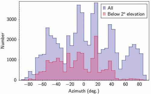
Figure 22. Distribution of aircraft following real flight paths within 1 hour of time in 5 degree azimuth sector towards Gatwick Airport received at Thurnham radar tower.

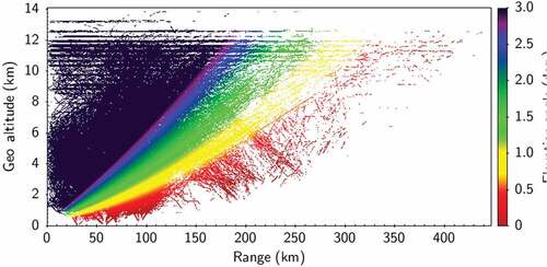
For the simulated humidity structure retrievals, the broadcasts were selected such that they spanned a suitable range in distance and altitude to effectively sample the extent of the lower atmosphere. The RH and mixing ratio vertical profiles had an altitude interval sufficiently small enough to show detailed structure. The initial RH vertical profile $x$ consisted of 574 RH values at height intervals of 0.02 km from an altitude of 0.12 km up to 11.98 km. In total, 2000 ADS-B messages were used, consisting of 68 unique aircraft ranging in altitude from 0.6 km to 11.6 km and in distance from 60 km to 205 km. This simulated study used real flight path data and a radiosonde-derived atmosphere to determine whether a theoretical ADS-B receiver positioned on a radar tower could observe enough refraction events to construct an estimate of the RH field.

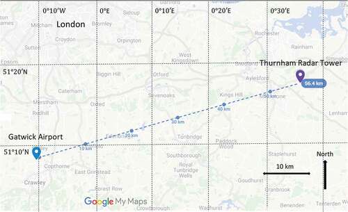
Figure 23 shows the distribution of the 2000 randomly chosen aircraft ADS-B messages in the $5$° azimuthal sector looking towards Gatwick Airport from Thurnham radar tower. The notional ADS-B interferometer was positioned at Thurnham radar tower (219 m altitude). This sector had a suitable distribution of broadcasts in both range and altitude, allowing for the atmosphere to be adequately sampled by ray-tracing methods. Figure 24 shows the position of Thurnham radar tower and Gatwick Airport located approximately 56 km to the southwest. The range 60 km to 205 km shows the path of aircraft taking off (if westerly winds were present) or descending to land (if easterly winds were present) at Gatwick Airport. The aircraft broadcast ADS-B messages throughout almost the entire extent of the troposphere, allowing for the vertical extent of the RH field to be determined. The temperature and atmospheric pressure were assumed to be known (derived from the Watnall, Nottinghamshire radiosonde data). The RH at every altitude grid point was initialized with the surface value of RH (in this case 73$\mathrm{\%}$). The simulated observed AoAs ranged from 0.1° and 3.1°. The density of broadcasts that can be used for humidity retrievals is highest in the lower atmosphere and decreases at higher altitudes ($\sim 9$ km is approximately cruising altitude for commercial aircraft). A theoretical ADS-B interferometer positioned at Thurnham radar tower could expect to observe hundreds of thousands of takeoffs and landings at Gatwick Airport every year (280.7 thousand takeoffs and landings were recorded in 2019, from https://www.statista.com/statistics/467333/aircraft-landings-and-take-offs-at-gatwick-airport-uk/), with each of these aircraft broadcasting thousands of ADS-B messages as they traverse the sky. The scale of observations, particularly in the lower atmosphere, would dramatically increase both the spatial and temporal resolution of RH/refractivity observations. A network of ADS-B interferometers across the UK could potentially allow for millions of RH/refractivity observations every day.

Figure 23. Distribution of aircraft used in the SA analysis. 68 unique aircraft were used and the number of broadcasts used in the analysis was 2000.

Figure 24. Map showing the location of Thurnham radar tower and Gatwick Airport. The distance between the two locations is approximately 56 km (from Google 2022.).

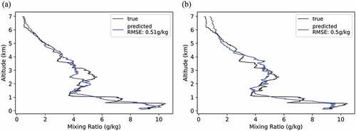
Figure 25(a) and Figure 25(b) show the true (black) RH vertical profiles at Watnall (determined by radiosonde) and the retrieved (blue) RH vertical profiles using the SA algorithm assuming a maximum AoA measurement noise of (a) 0.00° and (b) 0.01° respectively. The root mean squared error (RMSE) between the true RH values and the predicted RH values up to an altitude of 6 km were 4.6% and 4.7% for a maximum AoA measurement noise of 0.00° and 0.01° respectively. The SA algorithm was run for 1500 iterations using an initial temperature ${\beta }_0=10$ and a max step size $\mathrm{\Delta }{x}_{\mathrm{m}\mathrm{a}\mathrm{x}}=1.0\mathrm{\%}$. 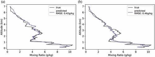Figures 26(a) and 26(b) show the true (black) mixing ratio vertical profiles at Watnall (determined by radiosonde) and the retrieved (blue) mixing ratio vertical profiles using the SA algorithm assuming a maximum AoA measurement noise of (a) 0.00° and (b) 0.01° respectively. The RMSE of the retrieved mixing ratio vertical profile up to an altitude of 6 km was 0.42 g/kg and 0.46 g/kg for a maximum AoA measurement noise of 0.00° and 0.01° respectively. The noise added to every AoA measurement was a random value in the range [$-{\delta }_{\mathrm{m}\mathrm{a}\mathrm{x}},{\delta }_{\mathrm{m}\mathrm{a}\mathrm{x}}$] (where ${\delta }_{\mathrm{m}\mathrm{a}\mathrm{x}}$ is the maximum AoA measurement noise) with a zero-mean Gaussian distribution. The retrieved RH vertical profile shows the most detailed structure near the surface, but appears to lose the signal generated by the true vertical profile at higher altitudes (above approximately 6 km). The corresponding mixing ratio vertical profiles show a significantly less extreme deviation from the true profile, indicating that the impact of water vapour on refraction at altitudes greater than approximately 6 km is minimal (also shown by the near-zero contribution of wet refractivity to the total refractivity in Figure 15).

Figure 25. (a) True RH vertical profile (black line) and the retrieved RH vertical profile (blue line) determined using the SA algorithm assuming a maximum AoA measurement noise of 0.00°. The true RH vertical profile was determined using the radiosonde data from Watnall at 11:15 UTC on the 27${ }^{\mathrm{t}\mathrm{h}}$ of July 2021. (b) True RH vertical profile (black line) and the retrieved RH vertical profile (blue line) determined using the SA algorithm assuming a maximum AoA measurement noise of 0.01°. The true RH vertical profile was determined using the radiosonde data from Watnall at 11:15 UTC on the 27${ }^{\mathrm{t}\mathrm{h}}$ of July 2021.

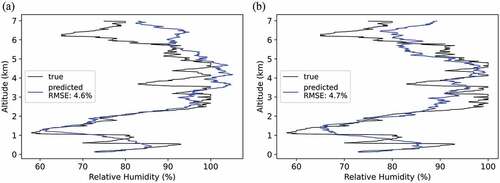
Figure 26. (a) True mixing ratio vertical profile (black) and the retrieved mixing ratio vertical profile (blue) determined using the SA algorithm assuming a maximum AoA measurement noise of 0.00°. The true mixing ratio vertical profile was determined using the radiosonde data from Watnall at 11:15 UTC on the 27${ }^{\mathrm{t}\mathrm{h}}$ of July 2021. (b) True mixing ratio vertical profile (black) and the retrieved mixing ratio vertical profile (blue) determined using the SA algorithm assuming a maximum AoA measurement noise of 0.01°. The true mixing ratio vertical profile was determined using the radiosonde data from Watnall at 11:15 UTC on the 27${ }^{\mathrm{t}\mathrm{h}}$ of July 2021.

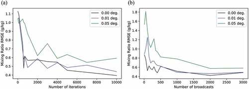
Figure 27(a) and Figure 27(b) show the dependence of the RMSE of the RH vertical profile retrieval (up to an altitude of 6 km) on the number of SA iterations (for 1500 broadcasts) and the number of broadcasts sampled (for 1500 iterations) respectively. The measurement noise of the AoA was assumed to be an uncorrelated random zero-mean Gaussian noise. The RMSE of both the RH and mixing ratio vertical profile retrievals were calculated up to an altitude of 6 km, since above this altitude the extremely low vapour pressure does not generate a strong enough signal to be detected. Increasing the number of iterations allows the SA algorithm to perform a more thorough search of the domain space for the global minimum, hence improving the quality of the retrieval. Figure 27(a) shows that for 1500 broadcasts the RMSE of the RH vertical profile retrieval after 10,000 iterations were 3.8%, 4.8% and 7.0% for a maximum AoA measurement noise of 0.00°, 0.01° and 0.05° respectively. The corresponding RMSE of the mixing ratio vertical profile retrieval for a maximum AoA measurement noise of 0.00°, 0.01° and 0.05° were 0.40, 0.44 and 0.59 g/kg respectively, as shown by Figure 28(a). For 1500 broadcasts the presence of a maximum AoA measurement noise of 0.05° significantly decreased the quality of the RH vertical profile retrieval compared to the maximum AoA measurement noise of 0.00° and 0.01°. However, above 3000 iterations, the RMSE of both the RH and mixing ratio vertical profile retrievals remained below 10.0% and 0.65 g/kg respectively. This is a problem of fitting to noisy data, where increasingly a background estimate of the RH/mixing ratio vertical profile must be known in order to weight each observation by its associated error. Increasing the number of broadcasts (sample points) allows for more of the RH/mixing ratio vertical profile to be sampled. For example, for a single ray path, there are a huge number of possible RH/mixing ratio vertical profiles that can cause the observed refraction. For two or more ray paths the potential RH/mixing ratio vertical profile must explain the refraction observed in all of the ray paths and thus is more constrained. Figure 27(b) shows that for 3000 broadcasts, the RMSE of the RH vertical profile retrieval was 5.0%, 5.4% and 6.1% for a maximum AoA measurement noise of 0.00°, 0.01° and 0.05° respectively. The corresponding RMSE of the mixing ratio vertical profile retrieval for the same maximum AoA measurement noise trials were 0.49, 0.49 and 0.58 g/kg respectively, as shown by Figure 28(b).

Figure 27. (a) The RMSE of the RH vertical profile retrieval up to 6 km altitude as a function of the number of iterations in the SA algorithm (for 1500 broadcasts) for different assumed maximum AoA measurement uncertainties. The initial temperature ${\beta }_0$ = 10 and max step size $\mathrm{\Delta }{x}_{\mathrm{m}\mathrm{a}\mathrm{x}}=1.0\mathrm{\%}$ were held constant. (b) The RMSE of the RH vertical profile retrieval up to 6 km altitude as a function of the number of broadcasts (for 1500 iterations) for different assumed maximum AoA measurement uncertainties. The initial temperature ${\beta }_0$ = 10 and max step size $\mathrm{\Delta }{x}_{\mathrm{m}\mathrm{a}\mathrm{x}}=1.0\mathrm{\%}$ were held constant.

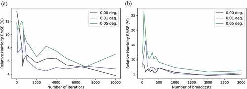
Figure 28. (a) The RMSE of the mixing ratio vertical profile retrieval up to 6 km altitude as a function of the number of iterations in the SA algorithm (for 1500 broadcasts) for different assumed maximum AoA measurement uncertainties. The initial temperature ${\beta }_0$ = 10 and max step size $\mathrm{\Delta }{x}_{\mathrm{m}\mathrm{a}\mathrm{x}}=1.0\mathrm{\%}$ were held constant. (b) The RMSE of the mixing ratio vertical profile retrieval up to 6 km altitude as a function of the number of broadcasts (for 1500 iterations) for different assumed maximum AoA measurement uncertainties. The initial temperature ${\beta }_0$ = 10 and max step size $\mathrm{\Delta }{x}_{\mathrm{m}\mathrm{a}\mathrm{x}}=1.0\mathrm{\%}$ were held constant.

Increasing the number of broadcasts showed the greatest reduction in RMSE of the retrieved RH/mixing ratio vertical profile. Assuming the noise in the AoA measurements has a zero-mean Gaussian distribution, increasing the number of broadcasts used in the retrieval means that the errors in individual broadcasts have a smaller impact on the quality of the retrieved vertical profile. These results indicate that if the uncertainties in the AoA measurements are maintained below $\sim 0.05$°, then vertical RH/mixing ratio profile retrievals with a RMSE of $\sim 5\mathrm{\%}$/$\sim 0.5$ g/kg respectively are possible. The SA algorithm is currently initialized assuming the RH is the same at every altitude, however, the speed of convergence to an optimum solution could potentially be improved by initializing the algorithm with a background estimate of the current profile (e.g. from a previous short term forecast). Variational analysis techniques could be used to consider the quality of the background estimate of the RH/mixing ratio vertical profile and ensure that very noisy measurements do not overwhelmingly impact the quality of the retrieval. It is envisioned that AoA measurements could be directly assimilated into NWP models in much the same way as bending angle measurements from radio-occultations are currently (Rennie 2010). Alternatively, the RH/refractivity measurements derived using SA (or other inversion techniques) could be assimilated into NWP models after pre-processing. However, the assimilation of refractivity determined from radio-occultation bending angle measurements above $\sim 30$ km can be problematic due to ’observed’ refractivity values above this altitude becoming increasingly influenced by information derived from climatology models (Healy 2008).

Figure 29(a) and Figure 29(b) show the RH vertical profile retrievals assuming a maximum measurement noise in the observed AoAs of 0.01° as well as assuming a vertical position uncertainty of (a) 10 m and (b) 15 m in the position of each aircraft. 2000 ADS-B messages were used, consisting of 68 unique aircraft ranging in altitude from 0.6 km to 11.6 km. These broadcasts were a random selection recorded assuming that the observer was positioned at Thurnham radar tower (219 m in altitude). The quality of the retrieval decreases significantly above an altitude of 6 km as the vertical position uncertainty increases from 10 m to 15 m, however, the major RH structures in the first few kilometres of the surface are still resolvable due to the larger contribution of the wet refractivity to the total refraction. Finer structures in the mixing ratio vertical profile are more difficult to resolve when assuming an uncertainty in the vertical position of the aircraft, however, the RMSE of the retrieved mixing ratio vertical profile is still comparable to the 0.01° maximum AoA measurement noise case. The SA algorithm was run for 1500 iterations using an initial temperature ${\beta }_0=10$ and max step size $\mathrm{\Delta }{x}_{max}=1.0\mathrm{\%}$. Figures 29(a) and 29(b) show that the RMSE of the retrieved RH vertical profile up to an altitude of 6 km was 5.1% and 5.6% for a vertical position uncertainty of 10 m and 15 m respectively. Figures 30(a) and Figure 30(b) show that the RMSE of the retrieved mixing ratio vertical profile up to an altitude of 6 km was 0.51 g/kg and 0.50 g/kg for a vertical position uncertainty of 10 m and 15 m respectively.

Figure 29. (a) True RH vertical profile (black) and the retrieved RH vertical profile (blue) determined using the SA algorithm assuming a maximum AoA measurement noise of 0.01° and a vertical position uncertainty of 10 m. The true RH vertical profile was determined using the radiosonde data from Watnall at 11:15 UTC on the 27^th of July 2021. True RH vertical profile (black) and the retrieved RH vertical profile (blue) determined using the SA algorithm assuming a maximum AoA measurement noise of 0.01° and a vertical position uncertainty of 15 m. The true RH vertical profile was determined using the radiosonde data from Watnall at 11:15 UTC on the 27^th of July 2021.

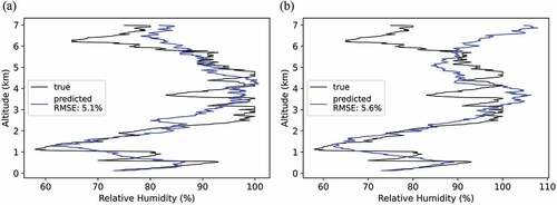
Figure 30. (a) True mixing ratio vertical profile (black) and the retrieved mixing ratio vertical profile (blue) determined using the SA algorithm assuming a maximum AoA measurement noise of 0.01° and a vertical position uncertainty of 10 m. The true mixing ratio vertical profile was determined using the radiosonde data from Watnall at 11:15 UTC on the 27^th of July 2021. (b) True mixing ratio vertical profile (black) and the retrieved mixing ratio vertical profile (blue) determined using the SA algorithm assuming a maximum AoA measurement noise of 0.01° and a vertical position uncertainty of 15 m. The true mixing ratio vertical profile was determined using the radiosonde data from Watnall at 11:15 UTC on the 27^th of July 2021.

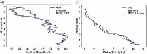
The SA retrieval algorithm was tested on two other RH and mixing ratio vertical profiles. Figure 31(a) shows the true (black, determined from radiosonde readings) and retrieved (blue) RH vertical profiles from Camborne at 11:24 UTC on the 26^th of July 2021. Figure 31(b) shows the corresponding mixing ratio vertical profiles. The RMSE of the RH and mixing ratio vertical profiles were $8.6\mathrm{\%}$ and 0.60 g/kg respectively. Figure 32(a) shows the true (black, determined from radiosonde readings) and retrieved (blue) RH vertical profiles from Camborne at 11:20 UTC on the 27^th of July 2021. Figure 32(b) shows the corresponding mixing ratio vertical profiles. The RMSE of the RH and mixing ratio vertical profiles were $6.2\mathrm{\%}$ and 0.41 g/kg respectively. The RH and mixing ratio vertical profiles were retrieved assuming that the observed AoA had a maximum measurement noise of $0.01$°. These results indicate that a variety of detailed RH and mixing ratio vertical profiles could be extracted using SA if the observed AoA uncertainty does not exceed $0.01$°.

Figure 31. (a) True RH vertical profile derived from radiosondes (black) and the retrieved RH vertical profile (blue) determined using the SA algorithm assuming a maximum AoA measurement noise of 0.01°. The true RH vertical profile was determined using the radiosonde data from Camborne at 11:24 UTC on the 26^th of July 2021. (b) True mixing ratio vertical profile derived from radiosondes (black) and the retrieved mixing ratio vertical profile (blue) determined using the SA algorithm assuming a maximum AoA measurement noise of 0.01°. The true mixing ratio vertical profile was determined using the radiosonde data from Camborne at 11:24 UTC on the 26^th of July 2021.

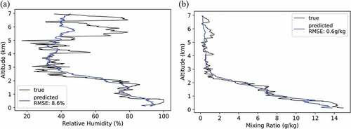
Figure 32. (a) True RH vertical profile derived from radiosondes (black) and the retrieved RH vertical profile (blue) determined using the SA algorithm assuming a maximum AoA measurement noise of 0.01°. The true RH vertical profile was determined using the radiosonde data from Camborne at 11:20 UTC on the 27${ }^{\mathrm{t}\mathrm{h}}$ of July 2021. (b) True mixing ratio vertical profile derived from radiosondes (black) and the retrieved mixing ratio vertical profile (blue) determined using the SA algorithm assuming a maximum AoA measurement noise of 0.01°. The true mixing ratio vertical profile was determined using the radiosonde data from Camborne at 11:20 UTC on the 27${ }^{\mathrm{t}\mathrm{h}}$ of July 2021.

6. Summary

A new method of retrieving atmospheric refractivity structure is proposed. It is mainly opportunistic, and has the potential to deliver large volumes of data at relatively low cost. Although the capital and running costs of an interferometer network would be modest, a substantial research and development effort is required for both hardware design and data exploitation. Experiments to date have focused on acquiring a basic technical capability with which to make some initial measurements, the first data look credible. This early success, combined with the scale of the potential benefits of any operational implementation, encourage the continuation of development. The horizontal errors due to latency in the ADS-B broadcast were found to likely only contribute slightly to the error in the reported AoA ($\sim {10}^{-3}$ deg.), whereas the uncertainty in the vertical position of the aircraft had the greatest contribution to the observed AoA error. For a 50 km source with a vertical position uncertainty of 15 m, the resulting uncertainty in the observed AoA was $\sim 0.03$°, exceeding the target resolution of 0.01°. Vertical relative humidity and mixing ratio profiles can be retrieved via refraction modelling and simulated annealing. The importance of minimizing the uncertainty in the AoA measurements has been demonstrated by the significant increase in the RMSE of the simulated relative humidity/mixing ratio vertical profile retrievals for AoA errors approaching 0.05°. The ability to retrieve relative humidity structures in the lower atmosphere exploits a current gap in high density humidity observations near the surface. With AoA measurement errors of $\sim 0.01$° the RMSE of the simulated retrieved relative humidity vertical profile up to 6 km altitude does not exceed 5$\mathrm{\%}$, which is within the WMO OSCAR breakthrough sensitivity requirement (WMO 2022.). The RMSE of less than 0.5 g/kg in the simulated retrieved mixing ratio vertical profile is comparable to/better than that retrieved using radio-occultation, which is generally in the range of 0.5–1.5 g/kg at 1000 hPa (Ho, Kuo, and Sokolovskiy 2007; Chen et al. 2014; Zhang et al. 2018; Ho and Peng 2018). The quality of the simulated retrieved mixing ratio vertical profile was comparable to those found by Gaffard et al. (2021) using a prototype Vaisala broadband differential absorption lidar (BB-DIAL) deployed at a Met Office research site. The RMSE in the retrieved mixing ratio vertical profile was 0.55 g/kg compared to in-situ observations of humidity (93 radiosonde ascents and 27 uncrewed aerial vehicle flights) and the Met Office UK Variable resolution model (UKV). However, the vertical retrieval capability of the BB-DIAL was rather limited, with an average maximum vertical extent of 1.3 km that could be probed. The simulated retrieval here has currently been restricted to only one dimension, however the quality of the retrievals even in the presence of noise is encouraging. It may be feasible to generalize the simulated annealing (SA) algorithm to two dimensions (including refractivity variations in the horizontal as well as vertical direction) and potentially three dimensions by including the azimuthal direction of received broadcasts. The technology can be adapted to existing radar tower infrastructure and early simulations using idealized and realistic model atmospheres indicate that the assimilation of AoA measurements could improve relative humidity/mixing ratio observations in the lower atmosphere in areas where there is a suitable density of air traffic. Current methods to measure humidity in the lower atmosphere suffer from a lack of resolution in both space and time: this new method of using AoA measurements could potentially dramatically increase the volume of humidity measurements in both space and time in areas with a suitable density of air traffic. However, the SA algorithm described here is computationally expensive and involves tracing many thousands of rays in order to calculate reported (unrefracted) AoAs. Work is also needed to reduce the observed errors in the AoAs measured using the prototype ADS-B interferometer, where simulated studies show that errors exceeding $0.01$° would significantly reduce the quality of the humidity retrieval.

Acknowledgment

We thank Neill Bowler and Ed Stone of the Met Office for their support in the creation of this paper and for collecting the ADS-B data from Thurnham radar tower. We would also like to thank the anonymous reviewer for their helpful and insightful comments that significantly improved the quality of the manuscript.

Disclosure statement

No potential conflict of interest was reported by the author(s).

Data availability statement

The radiosonde data that support the findings of this study are available in ‘Met Office (2006): Met Office high resolution radiosonde data from the UK, Gibraltar, St Helena and the Falkland Islands’, CEDA Archive at http://catalogue.ceda.ac.uk/uuid/c1e2240c353f8edeb98087e90e6d832e. (Accessed 10 May 2022).

Correction Statement

This article has been corrected with minor changes. These changes do not impact the academic content of the article.

Additional information

Funding

The work was supported by the University of Exeter (College of Engineering, Mathematics and Physical Sciences) and Met Office [118558].

References

- Bengtsson, L., and K. I. Hodges. 2005. “On the impact of humidity observations in numerical weather prediction.” Tellus A: Dynamic Meteorology and Oceanography 57 (5): 701–708. doi:10.3402/tellusa.v57i5.14734.
- Bennitt, G. V., and A. Jupp. 2012. “Operational Assimilation of GPS Zenith Total Delay Observations into the Met Office Numerical Weather Prediction Models.” Monthly Weather Review 140 (8): 2706–2719. doi:10.1175/MWR-D-11-00156.1.
- Bizzarri, B., I. Bordi, A. Dell’aquila, M. Petitta, and A. Sutera. 2004. “GPS radio occultation sounding to support General Circulation Models.” Il Nuovo Cimento 27 (1): 59–71. doi:10.1393/ncc/i2004-10007-1.
- Buck, A. L. 1996. “Buck Research CR-1A User’s Manual, Appendix 1.”
- Chen, S. Y., T. K. Wee, Y. H. Kuo, and D. H. Bromwich. 2014. “An Impact Assessment of GPS Radio Occultation Data on Prediction of a Rapidly Developing Cyclone over the Southern Ocean.” Monthly Weather Review 142 (11): 4187–4206. doi:10.1175/MWR-D-14-00024.1.
- de Haan, S. 2008. Meteorological applications of a surface network of Global Positioning System receivers. Wageningen, Netherlands: Wageningen University and Research. https://www.knmi.nl/kennis-en-datacentrum/publicatie/meteorological-applications-of-a-surface-network-of-global-positioning-system-receivers
- de Haan, S., M. de Haij, and J. Sondij. 2013. The Use of a Commercial ADS-B Receiver to Derive Upper Air Wind and Temperature Observations from Mode-S EHS Information in the Netherlands. TR-336. De Bilt, Netherlands: KNMI.
- Fabry, F., C. Frush, I. Zawadzki, and A. Kilambi. 1997. “On the Extraction of Near-Surface Index of Refraction Using Radar Phase Measurements from Ground Targets.” Journal of Atmospheric and Oceanic Technology 14 (4): 978–987. doi:10.1175/1520-0426(1997)014<0978:OTEONS>2.0.CO;2.
- Faragher, R., P. F. MacDoran, and M. B. Mathews. 2014. “Spoofing Mitigation, Robust Collision Avoidance, and Opportunistic Receiver Localisation Using a New Signal Processing Scheme for ADS-B or AIS.” In Proceedings of the 27th International Technical Meeting of The Satellite Division of the Institute of Navigation (ION GNSS+2014), Tampa, Florida, USA, 858–868.
- Gaffard, C., Z. Li, D. Harrison, R. Lehtinen, and R. Roininen. 2021. “Evaluation of a Prototype Broadband Water-Vapour Profiling Differential Absorption Lidar at Cardington, UK.” Atmosphere 12 (11): 1521. doi:10.3390/atmos12111521.
- Geer, A. J., F. Baordo, N. Bormann, P. Chambon, S. J. English, M. Kazumori, H. Lawrence, P. Lean, K. Lonitz, and C. Lupu. 2017. “The growing impact of satellite observations sensitive to humidity, cloud and precipitation.” Quarterly Journal of the Royal Meteorological Society 143 (709): 3189–3206. doi:10.1002/qj.3172.
- Google (My Maps). 2022. ”Thurnham View of Gatwick”. Accessed 10 May 2022. https://www.google.com/maps/d/viewer?mid=1wkp_toO97E9pKylnAruyq09ThjjZUzhK&usp=sharing
- Haase, J. S., B. J. Murphy, P. Muradyan, F. G. Nievinski, K. M. Larson, J. L. Garrison, and K. N. Wang. 2014. “First results from an airborne GPS radio occultation system for atmospheric profiling.” Geophysical Research Letters 41 (5): 1759–1765. doi:10.1002/2013GL058681.
- Hayward, R., and A. Price. 2015. General Aviation: ADS-B/GPS Trial Results. Fareham, Hampshire, UK: NATS.
- Healy, S. B. 2008. “Assimilation of GPS radio occultation measurements at ECMWF.” In Proceedings of the GRAS SAF Workshop on Applications of GPSRO measurements, ECMWF, Reading, UK, ECMWF, 16–18.
- Ho, S. P., Y. H. Kuo, and S. Sokolovskiy. 2007. “Improvement of the Temperature and Moisture Retrievals in the Lower Troposphere Using AIRS and GPS Radio Occultation Measurements.” Journal of Atmospheric and Oceanic Technology 24 (10): 1726–1739. doi:10.1175/JTECH2071.1.
- Ho, S. P., and L. Peng. 2018. “Global Water Vapor Estimates from Measurements from Active GPS RO Sensors and Passive Infrared and Microwave Sounders.“ Green Chemistry Applications, edited byM. Eyvaz, and E. Yüksel. Rijeka, Croatia: IntechOpen. doi:10.5772/intechopen.79541.
- ICAO. 2013. “Global Navigation Satellite System (GNSS) Manual.” International Civil Aviation Organization Doc 9849 (AN/457): 90.
- Kamineni, R., T. N. Krishnamurti, R. A. Ferrare, S. Ismail, and E. V. Browell. 2003. “Impact of High Resolution Water Vapor Cross-Sectional Data on Hurricane Forecasting.” Geophysical Research Letters 30: 5. doi:10.1029/2002GL016741.
- Kerr, D. E. 1987. Propagation of short radio waves (Revised edition). Vol. 24 IEE Electromagnetic Waves Series. London, UK: Peter Peregrinus Ltd. / IEE.
- Kuo, Y. H., S. V. Sokolovskiy, R. A. Anthes, and F. Vandenberghe. 2000. “Assimilation of GPS Radio Occultation Data for Numerical Weather Prediction.” Terrestrial Atmospheric and Oceanic Sciences 11 (1): 157–186. doi:10.3319/TAO.2000.11.1.157(COSMIC).
- Liu, Z., S. Lo, and T. Walter. 2020. “Characterization of ADS-B Performance Under GNSS Interference.“ Proceedings of the 33rd International Technical Meeting of the Satellite Division of The Institute of Navigation (ION GNSS+ 2020), 3581–3591.
- Martin F. L. and Wright F. E. (1963). Radar-ray refraction associated with horizontal variations in the refractivity. Journal of Geophysical Research, 68(7), 1861–1869. doi:10.1029/JZ068i007p01861.
- Menke, W. 2018. Geophysical Data Analysis: Discrete Inverse Theory (Fourth Edition). Cambridge, Massachusetts, USA: Elsevier Academic Press. doi:10.1016/C2016-0-05203-8.
- Rennie, M. P. 2010. “The impact of GPS radio occultation assimilation at the Met Office.” Quarterly Journal of the Royal Meteorological Society: A Journal of the Atmospheric Sciences, Applied Meteorology and Physical Oceanography 136 (646): 116–131. doi:10.1002/qj.521.
- RTCA. 2011. 2608 Minimum Operational Performance Standards for 1090MHz Extendedsquitter Automatic Dependent Surveillance-Broadcast (ADS-B) and Traffic Information Service-Broadcast (TIS-B). Washington DC, USA: RTCAInc.
- Smith, E. K., and S. Weintraub. 1953. “The Constants in the Equation for Atmospheric Refractive Index at Radio Frequencies.” Proceedings of the IRE 41 (8): 1035–1037.
- Solheim, F. S., J. Vivekanandan, R. H. Ware, and C. Rocken. 1999. “Propagation delays induced in GPS signals by dry air, water vapor, hydrometeors, and other particulates.” Journal of Geophysical Research Atmospheres 104 (D8): 9663–9670. doi:10.1029/1999JD900095.
- Stone, E. K., and M. Kitchen. 2015. “Introducing an Approach for Extracting Temperature from Aircraft GNSS and Pressure Altitude Reports in ADS-B Messages.” Journal of Atmospheric and Oceanic Technology 32 (4): 736–743. doi:10.1175/JTECH-D-14-00192.1.
- Stone, E. K., and G. Pearce. 2016. “A Network of Mode-S Receivers for Routine Acquisition of Aircraft-Derived Meteorological Data.” Journal of Atmospheric and Oceanic Technology 33 (4): 757–768. doi:10.1175/JTECH-D-15-0184.1.
- Verbraak, T., J. Ellerbroek, J. Sun, and J. Hoekstra. 2017. “Large-Scale ADS-B Data and Signal Quality Analysis.” In Proceedings of the 12th USA/Europe Air Traffic Management Research and Development Seminar, Seattle, Washington, USA.
- Vowles, M. C. 2007. “An investigation of tropospheric refractive effects on Ka-band terrestrial links.” PhD diss. Bath, UK, University of Bath.
- Wadge, G., A. Costa, K. Pascal, C. Werner, and T. Webb. 2016. “The Variability of Refractivity in the Atmospheric Boundary Layer of a Tropical Island Volcano Measured by Ground-Based Interferometric Radar.” Boundary-Layer Meteorology 161 (2): 309–333. doi:10.1007/s10546-016-0168-3.
- Wallace, J. M., and P. V. Hobbs. 2006. Atmospheric Science: An Introductory Survey. Vol. 92. Cambridge, Massachusetts, USA: Elsevier Academic Press.
- Watson, R. J., and C. J. Coleman. 2010. “The Use of Signals of Opportunity for the Measurement of Atmospheric Refractivity.” In Proceedings of the Fourth European Conference on Antennas and Propagation, Barcelona, Spain, 1–5. IEEE.
- Weckwerth, T. M., C. R. Pettet, F. Fabry, S. J. Park, M. A. LeMone, and J. W. Wilson. 2005. “Radar Refractivity Retrieval: Validation and Application to Short-Term Forecasting.” Journal of Applied Meteorology 44 (3): 285–300. doi:10.1175/JAM-2204.1.
- WMO. 2022. ”Observing Systems Capability Analysis and Review Tool.” Accessed 10 May 2022. https://space.oscar.wmo.int/
- Zhang, Q., J. Ye, S. Zhang, and F. Han. 2018. “Precipitable Water Vapor Retrieval and Analysis by Multiple Data Sources: Ground-Based GNSS, Radio Occultation, Radiosonde, Microwave Satellite, and NWP Reanalysis Data.” Journal of Sensors 2018. doi:10.1155/2018/3428303.
- Zhao, Q., K. Zhang, and W. Yao. 2019. “Influence of station density and multi-constellation GNSS observations on troposphere tomography.” In Annales Geophysicae. Vol. 37, 15–24. Göttingen, Germany: Copernicus. doi:10.5194/angeo-37-15-2019.