Performance evaluation of convolution neural networks in canopy height estimation using sentinel 2 data, application to Thailand

ABSTRACT

Electric shorting induced by tall vegetation is one of the major hazards affecting power transmission lines extending through rural regions and rough terrain for tens of kilometres. This raises the need for an accurate, reliable, and cost-effective approach for continuous monitoring of canopy heights. This paper proposes and evaluates two deep convolution neural network (CNN) variants based on Seg-Net and Res-Net architectures, characterized by their small number of trainable weights (nearly 800,000) while maintaining high estimation accuracy. The proposed models utilize the freely available data from Sentinel-2, and a digital surface model to estimate forest canopy heights with high accuracy and a spatial resolution of 10 metres. Various factors affect canopy height estimation, including topography signature, dataset diversity, input layers, and model structure. The proposed models are applied separately to two powerline regions located in the northern and southern parts of Thailand. The application results show that the proposed Encoder-Decoder CNN Seg-Net model presents an average mean absolute error (MAE), root mean square error (RMSE), and coefficient of determination $\left(R^2\right)$ of 1.38 m, 1.85 m, and 0.87, respectively, and is nearly 4.8 times faster than the CNN Res-Net model in conversion. These results prove the proposed model’s capability of estimating and monitoring canopy heights with high accuracy and fine spatial resolution.

KEYWORDS:

• Forest Structure
• Encoder-Decoder
• High Resolution
• remote sensing
• Feature Importance

1. Introduction

Forest canopy height is one of the most significant parameters used to characterize a forest’s structure, which is an important indicator of several ecosystem functions such as forest above-ground biomass (Zhao, Popescu, and Nelson 2009), species diversity (Zhao et al. 2018), forest productivity (Gholz, Nakane, and Shimoda 2012), and carbon storage (Myeong, Nowak, and Duggin 2006). Furthermore, it is used in risk management, such as forest fire risk analysis (Gale et al. 2021), as well as the topic of this paper: estimating forest encroachment across power transmission lines, which is a serious electric shorting hazard in tropical regions like Thailand. The power transmission lines usually extend for several tens of kilometres to transmit electric power from power plants to consumption areas. These circumstances render visual inspection and in-situ direct observations of tree heights ineffective due to their limited coverage, sparse revisit times, high cost, and labour requirements. Airborne light detection and ranging (LiDAR) has the capability of mapping canopy heights with high accuracy. However, this technique is highly expensive, and its spatial coverage is limited, which inhibits its usability for regular monitoring of hazardous regions.

These shortcomings draw attention to remote sensing techniques for estimating forest canopy heights. Cloude and Papathanassiou (1998) proposed using a fully Polarimetric Interferometric Synthetic Aperture Radar (Pol-InSAR) to generate and optimize a complex coherency matrix using single-value decomposition. As a result, two distinct phase scattering centres related to the canopy’s top and ground were identified, which are used to estimate the forest canopy height by complex conjugating the phase of these scattering centres and dividing by the SAR vertical wave number.This methodology was pristine and promising and was further matured into the Random Volume over Ground (RVoG) model (Papathanassiou and Cloude 2001) and the three-stage technique to facilitate the model’s inversion (Cloude and Papathanassiou 2003). This technique has been improved by numerous researchers using full and dual polarimetric SAR observations, for example (Lavalle, Simard, and Hensley 2011; Wenxue et al. 2015). However, these techniques come with challenges. For instance, the RVoG model relies on the vertical wavenumber, which is determined by the sensor’s flying height and the normal baseline between SAR acquisitions. As a result, the small vertical wavenumber of spaceborne SAR makes measurements particularly sensitive to phase noise and reduces accuracy (Kugler et al. 2015). In addition, coherence estimation requires a multi-looking and ensemble estimating window, lowering spatial resolution significantly. Furthermore, the temporal decorrelation generated by the time interval between satellite SAR observations renders the phase useless for the C and X bands and reduces the accuracy of the L-band significantly. These are some of the reasons why the Pol-InSAR approach is best suited for aerial SAR observations rather than spaceborne ones, which makes this technology ineffective for continuous monitoring of forest canopy heights because it suffers from the same limitations as LiDAR observation, namely the high cost of the observation plane and its limited coverage.

Several novel technological breakthroughs have recently been introduced, such as cloud-based processing and the availability of petabytes of space remote sensing datasets. One of the first and most advanced online remote sensing tools is Google Earth Engine (GEE) (Gorelick et al. 2017), which has a massive and constantly updated dataset. In addition to Google Colaboratory (Bisong 2019), a Python-based online processing environment, and user-friendly machine learning libraries like TensorFlow (TF) (https://tensorflow.org) and Keras (https://keras.io). This inspired many researchers to study the potential of these unprecedented capabilities in a variety of remote sensing applications, including forest canopy height.

Artificial Neural Network (ANN) architectures contain numerous minute characteristics that set them apart. As a result, the most acknowledged studies on this subject are presented, along with information about the used data, the type of ANN architecture, the spatial resolution, and the reported accuracy (Table 1). Almost all the reported studies employ aerial LiDAR data as a ground truth estimate of canopy heights for ANN training, and a few use spaceborne LiDAR data, such as ICESat-2. Hansen et al. (2016) mapped tree height distribution in Sub-Saharan Africa using four bands of Landsat 7 and Landsat 8 data and a network of seven bagged tree models with a spatial resolution of 30 metres and a Mean Absolute Error (MAE) of 4.65 metres for trees over 20 metres. Lang, Schindler, and Wegner (2019) used a deep convolution neural network (CNN) of 18 neural blocks with skip connections called SepConv, employing thirteen bands of Sentinel-2 data to map vegetation heights in Switzerland and Gabon with RMSEs of 3.4 and 5.6 metres, respectively. Li et al. (2020) developed deep learning (DL) and random forest (RF) models using Sentinel 1, Sentinel 2, Landsat 8, and spectral indices to generate tree height maps with spatial resolutions ranging from 10 to 1000 metres, with an RMSE of 2.39 metres at 250 spatial resolution. Aamir et al. (2020) employed eleven bands of Landsat 8 data and nineteen spectral indices to estimate forest canopy heights in Arizona, U.S.A, using CNN with a spatial resolution of 30 metres and an MAE of 3.09 metres. Alagialoglou et al. (2021) used twelve bands of Sentinel 2 data to estimate forest canopy height in Germany and the Czech Republic using an encoder-decoder model based on CNN with a spatial resolution of 10 metres and a RMSE of 3.15 metres. Liu et al. (2022) used the Global Ecosystem Dynamics Investigation (GEDI), ICESat-2, airborne lidar, and Normalized Difference Vegetation Index (NDVI) to estimate forest canopy height in China using a neural network guided interpolation (NNGI) model with a spatial resolution of 30 metres and a RMSE of 4.88 metres.

Table 1. Published models for forest height estimation using artificial neural network.

Region of application	Dataset	Number of input features	Model used	Spatial Resolution (m)	MAE (m)	RMSE (m)	Reference
Sub-Saharan Africa	Landsat 7 Landsat 8	4 bands	seven bagged tree models	30	4.65	Not reported	Hansen et al. (2016)
Switzerland and Gabon	Sentinel 2	13 bands	CNN − 18 SepConv blocks	10	1.7, 4.3	3.4, 5.6	Lang, Schindler, and Wegner (2019)
Mongolia, China	Sentinel 1 Sentinel 2 Landsat 8 ICESat-2	22 bands and spectral indices	DL and RF	10, 30, 250, 500, 1000	3.22, 2.86, 2.39, 2.58, 3.21	Not reported	Li et al. (2020)
Arizona, U.S.A	Landsat 8	11 bands and 19 spectral indices	CNN	30	3.09	Not reported	Aamir et al. (2020)
Germany, Czech Republic	Sentinel 2	12 bands	ConvEnc-DecSkip	10	2.29	3.15	Alagialoglou et al. (2021)
China	Sentinel 2 GEDI ICESat-2	NDVI LiDAR data	NNGI	30	Not reported	4.88	Liu et al. (2022)

This research is motivated by the need for a reliable technique for continuous and fast response monitoring of forest canopy heights across power transmission lines, which is a significant hazard source, especially in tropical regions characterized by heavy rain and dense forests like Thailand. Several challenges were identified during this research: (1) the powerlines extend through forested, agricultural, rural, and urban regions, which makes the canopy heights highly non-uniform as they change from nearly 1 metre directly under the power lines to more than 30 metres within 10 metres from either side of the power lines; (2) tropical atmospheric conditions and heavy cloud cover obscure clear observations of the canopies; and (3) rough and forested terrain casts variant shadows, which change the spectral reflectance of the observed canopies.

To overcome these challenges, we study and evaluate two of the most used convolution neural network architectures in raster regression, namely: SegNet (Alagialoglou et al. 2021), and ResNet, (Lang, Schindler, and Wegner 2019). Then, we propose our deep convolution neural network variants of the two architectures, characterized by their small number of trainable weights while maintaining high estimation accuracy. The proposed architectures utilize the freely available data of Sentinel-2, and ALOS Global DSM (AW3D30), which produce an estimate of the forest canopy height with a spatial resolution of 10 metres and an MAE of less than 1.7 metres. To identify the best data-model combination that ensures the required height estimation accuracy while maintaining a discrete dataset, we examined numerous neural network variants and reported the best parameters for our study region. Moreover, we study two distinct powerline regions, one in the northern part of Thailand and the second in the southern part (Figure 1). The two regions are mutually different in terrain, canopy height distribution, and atmospheric conditions. This diversity in study region characteristics allows for quantifying and estimating their effects on the expected canopy height estimation accuracy using the proposed models. Additionally, this research presents a significant analysis of the input layers and the identification of the most effective input data to reduce the amount of dataset processing and facilitate canopy height estimation.

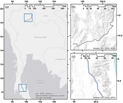
Figure 1. (A) Location of study regions in Thailand, (b) Northern power transmission line, and (c) Southern power transmission line.

2. Study region and dataset

2.1. Study region

The proposed models were applied to two powerline regions (Figure 1a). The first powerline is in the northern part of Thailand, extending from Lampang to Nan provinces and passing through Phrae province (Figure 1b), with a total length of 208 kilometres and an average analysis width of 900 metres, covering an approximate area of 187 square kilometres. The second powerline is in the southern part of Thailand, extending from Surat Thani to Nakhon Si Thammarat provinces (Figure 1c), with a total length of 123 kilometres and an average analysis width of 1600 metres, covering an approximate area of 197 square kilometres.

The selected regions are characterized by their tropical climate, rainy weather, and dense cloud cover. The terrain varies from nearly flat vegetated and bare land to rugged, rough, and forested mountainous terrain. Vegetation heights range from one metre in agricultural areas to nearly thirty metres in forested areas. The selected study regions exemplify the various challenges facing accurate forest height estimation.

Canopy heights and topographic features’ normalized histograms and probability density functions (PDFs) are presented in Figure 2 for both study regions. It shows that the average canopy heights in the northern region are smaller than those in the southern region (Figure 2a), with average heights of 4.96 and 8.64 metres, respectively (Table 2). The data show a large difference in the DSM elevation between the study regions (Figure 2b). The northern region has a higher elevation with a mean value of 297.61 metres, while the southern region has a lower elevation with a mean value of 40.18 metres (Table 2). Also, the northern region shows a higher DSM slope variation with a mean and standard deviation of 10.65 and 7.96 degrees, respectively, compared to the southern region, which shows a milder topography and DSM slope variation with a mean and standard deviation of 4.82 and 4.54 degrees, respectively (Figure 2c) (Table 2). Meanwhile, the DSM aspect variation for both study regions shows the same statistical characteristics (Figure 2d).

Figure 2. Normalized histograms and PDFs of the study regions, (a) LiDAR canopy heights, (b) DSM elevation, (c) DSM slope, (d) DSM aspect.

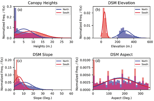
Table 2. Statistical details of canopy heights and topographic conditions in study regions.

	Canopy Height (m.)		DSM Elevation (m.)		DSM Slope (Deg.)		DSM Aspect (Deg.)
Region	North	South	North	South	North	South	North	South
Max	29.44	39.66	637.21	213.99	62.56	71.25	359	358
Min	0	0	167.97	−28.00	0	0	0	0
μ	4.96	8.64	297.61	40.18	10.65	4.82	173	166
σ	±4.59	±6.10	±68.60	±19.09	±7.96	±4.54	±99.4	±106.6

μ: Data mean value, σ: Data standard deviation.

2.2. Datasets

For the dataset, we utilized all 12 bands of the Sentinel-2 satellite images, and AW3D30 DSM, in addition to 27 different spectral indices and parameters derived from the observed data, which makes a total of 40 input layers to the ANN model (Table A1), in addition to airborne LiDAR canopy height data for model training.

2.2.1. Airborne LiDAR data

The proposed models are trained and evaluated using airborne LiDAR data provided by the Electricity Generating Authority of Thailand (EGAT). The airborne LiDAR data was collected in November and February, 2016, for the northern and southern powerlines, respectively, with a spatial resolution of 50 centimetres (Table 3). After obtaining an initial estimate of forest canopy heights, we remove any anomalous pixels caused by an error during LiDAR processing or representing urban regions. Then, we align and down sample the LiDAR data to 10 m resolution using the average module to match the Sentinel-2 data’s resolution and projection.

Table 3. Dataset details.

Data Type	Observation Times		Number of Bands	Spatial Resolution (m)
	Northern Powerline	Southern Powerline
LiDAR Data	November 2016	February 2016	1	0.5
Sentinel-2 (1C)	[1, 8, 18, 21] November 2016	[5, 12] February 2016	13	10/20/60
AW3D30	2006: 2011	2006: 2011	1	30

2.2.2. Sentinel-2 dataset

Sentinel-2 (S-2) is a European wide-swath, high-resolution, multi-spectral imaging mission in the Copernicus programme of the European Space Agency (ESA) (https://sentinel.esa.int). It consists of two polar-orbiting satellites placed in the same sun-synchronous orbit and phased at 180° to each other. Sentinel-2 is equipped with an optical instrument payload with an orbital swath of 290 kilometres wide that samples 13 spectral bands: four at 10 m, six at 20 m, and three at 60 m spatial resolution. Starting in late June 2015, the Level 1C data product includes top-of-atmosphere (TOA) reflectance, while the Level 2A data product includes bottom-of-atmosphere (BOA) reflectance beginning in late March 2017. The data products are organized in 100 × 100 km² georeferenced tiles in UTM/WGS84 projection.

The dataset archives for the products are available for cloud processing and downloading from Google Earth Engine’s (GEE) platform (Gorelick et al. 2017). However, because the LiDAR’s data falls outside the Level (2A) ready-to-use archive, we downloaded all the available Level (1C) data (Table 3) from the Copernicus open access hub (https://scihub.copernicus.eu/) and processed it to obtain the 12 bands (BOA) Level (2A) product (Table A1) using Sen2Cor v2.10 (Main-Knorn et al. 2017), a standalone Sentinel-2 data processor. Then, the cloud mask band was used to remove the cloud-affected pixels and generate a cloud-free 12-band image (Table A1). The bands with spatial resolutions of 20 and 60 metres were bilinearly up-sampled to a spatial resolution of 10 metres. Then, 25 spectral indices were included in the ANN models to test their performance and identify the most effective input feature layers (Table A1).

The final preprocessing step is normalizing the input feature layers across the whole dataset to speed up the model’s convergence, which makes the input values range between [0: 1] or [−1: 1], Equation (1)(1) $X_{i,norm}=\frac{X_i-min\left(X\right)}{max\left(X\right)-min\left(X\right)}$(1) . However, for the S-2 (2A) bands, the maximum value does not exceed 10,000 and the minimum value is zero; therefore, we simply multiply the values of the S-2 bands by 0.0001 for normalization. Additionally, some spectral index values already range between [−1: 1], e.g. the NDVI; therefore, they are included in the model without any change. Any other feature layer that has values outside the [−1: 1] range is normalized using Equation (1)(1) $X_{i,norm}=\frac{X_i-min\left(X\right)}{max\left(X\right)-min\left(X\right)}$(1) .

(1) $X_{i,norm}=\frac{X_i-min\left(X\right)}{max\left(X\right)-min\left(X\right)}$(1)

where $X$ is a feature input layer, and $X_{i,norm}$ is the value after normalization. This dataset contributes 37 input feature layers to the proposed ANN model.

2.2.3. AW3D30 dsm

The ALOS World 3D 30 m (AW3D30) dataset (Takaku, Tadono, and Tsutsui 2014) is a global digital surface model (DSM) with a horizontal resolution of about 30 metres. The dataset is based on the World 3D Topographic Data (5-metre version). The elevation of the AW3D DSM is calculated using an image-matching process that employs a stereo pair of optical images observed by the ALOS-Prism sensor, which was launched in January 2006 by the Japan Aerospace Exploration Agency (JAXA) and was decommissioned in May 2011. The AW3D30 data was obtained from GEE’s archives (Table 3), then the slope and aspect of each pixel were calculated. Because the data has a spatial resolution of 30 metres, it was bi-linearly up-sampled to a spatial resolution of 10 metres and normalized with Equation (1)(1) $X_{i,norm}=\frac{X_i-min\left(X\right)}{max\left(X\right)-min\left(X\right)}$(1) . This procedure resulted in the addition of three input feature layers to the proposed ANN model, (Table A1).

3. Methodology

3.1. Neural network architectures

During this research, several regression approaches were evaluated for estimating canopy heights, and it was found that Convolution Neural Networks (CNNs) are the best ANN technique in terms of accuracy, model conversion, and generalization. The basic principle of CNNs is to extract specific features from image bands by convolving the input feature layers with a set of two-dimensional convolution filter kernels followed by an activation function. This operation can be repeated several times with chosen variations according to the proposed ANN design, yielding a deep network that gradually transforms the input feature layers to the desired output values. During model training, the parameters of the convolution filter kernels are directly learned from the input data and continuously adjusted in each training iteration to increase the model’s accuracy. This study proposes two architecture variants of the CNN technique that are characterized by their small number of trainable weights while maintaining high estimation accuracy. The research applies the two models to the same study regions and evaluates their performance.

3.1.1. CNN based on segnet

The first proposed model is an Encoder-Decoder Seg-Net architecture based on CNNs (Figure 3a). The model starts by reading the input dataset after dividing it into non-overlapping patches with a size of (24 by 24 pixels by M), where M is the number of input layers, which equals 40 in full dataset analysis. Then, the data is passed to a basic analysis block, which consists of (1) 2D-Convolution layer with a size of (3, 3, N), where N is the number of linear filter kernels, (2) a rectified linear unit activation function (ReLU) that clips negative values and passes positive ones, and (3) a batch normalization layer that standardizes the layers’ inputs to stabilize the learning process and reduce the number of required training epochs. Additional layers are added to the basic analysis block as needed, such as (4) a 2D-Maxpooling layer to reduce the number of training parameters by selecting the highest values within a 2 by 2 moving window with a step of 2 pixels (stride of 2), (5) a dropout layer that randomly drops out nodes during model training, which offers a very computationally effective regularization to reduce the model’s overfitting and improve generalization error, and (6) a 2D-Upsample layer that increases the size of the feature map to retain the original size before the 2D-Maxpooling.

Figure 3. Architecture of the proposed CNN models, (a) an Encoder-Decoder Seg-Net model, (b) a Res-Net model.

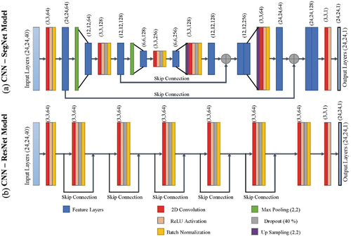
In the Encoder stage, (Figure 3a), the dataset (24, 24, 40) is passed to the basic analysis block with a 2D convolution layer with a size of (3, 3, N = 64), resulting in a feature map number (1) with a size of (24, 24, 64) after batch normalization. Then, feature map number (1) is passed to a 2D-Maxpooling layer, resulting in feature map number (2) with a size of (12, 12, 64), which is passed to a second basic analysis block with a 2D convolution layer with the size of (3, 3, 2N = 128), and an additional (40%) Dropout layer before the batch normalization layer. The resulting feature map number (3) with a size of (12, 12, 128) is passed to a 2D-Maxpooling layer, resulting in feature map number (4) with a size of (6, 6, 128). Feature map number (4) is passed to a third basic analysis block with a 2D convolution layer with a size of (3, 3, 4N = 256) and a (40%) Dropout layer, resulting in feature map number (5) with a size of (6, 6, 256), which is called the bottleneck of the network.

In the Decoder stage, (Figure 3a), the feature map number (5) is passed to a 2D-Upsample layer, then to a fourth basic analysis block with a 2D convolution layer with a size of (3, 3, 2N = 128) and a (40%) Dropout layer, resulting in feature map number (6) with a size of (12, 12, 128). Then, feature maps (3) and (6) are concatenated and passed to a 2D-Upsample layer and a fifth basic analysis block with a 2D convolution layer of size (3, 3, N = 64), yielding feature map number (7) of size (24, 24, 64). Then, feature maps numbers (1) and (7) are concatenated and passed to a 2D convolution layer with a size of (3, 3, N = 1) and a ReLU activation layer, resulting in the final canopy heights map with a size of (24, 24, 1).

In this research, we tested numerous variations of the Encoder-Decoder ANN model architecture and we found that when reducing the network bottleneck 2D size to less than (6, 6), the final accuracy of the model is reduced because the information neglected during the 2D-Maxpooling stage could not be retrieved, which affects the final model accuracy. This is the reason for using the skip connection to concatenate Encoder feature maps with Decoder feature maps to retain and preserve the important information neglected during the 2D-Maxpooling and dropout layers.

3.1.2. CNN based on ResNet

The second proposed model is a Res-Net architecture based on CNNs (Figure 3b). The model starts by reading the input dataset after dividing it into non-overlapping patches with a size of (24 by 24 pixels by M), where M equals 40 in full dataset analysis. Then, the data is passed to an entry analysis block, which consists of (1) 2D-Convolution layer with a size of (3, 3, N), (2) a rectified linear unit activation function (ReLU), and (3) a batch normalization layer. Then, the data is passed through five consecutive and identical CNN blocks with a skip layer on each and consists of (1) 2D-Convolution layer with a size of (3, 3, N), (2) a ReLU function, (3) a 40% Dropout layer, and (4) a batch normalization layer. Then, the data is passed through an additional CNN block without the skip layer, and then it passes through an exit CNN block, which consists of a 2D convolution layer with a size of (3, 3, N = 1) and a ReLU activation layer, resulting in the final canopy heights map with a size of (24, 24, 1).

3.2. Model learning and evaluation

The proposed Seg-Net and Res-Net networks have (837,121) and (798,593) trainable weights, respectively, when using the full 40 layers dataset and a 2D convolution layer with linear filter kernels of (N = 64). Since the canopy height estimation is a continuous regression problem, we selected to minimize a $\left(L_1-Loss\right)$ function (i.e. mean absolute error) to train the model parameters, Equation (2)(2) $MAE=\frac{1}{n}{\sum }_{i=1}^n\left|f\left(x_i\right)-y_i\right|$(2) , mainly because $L_1$ function has the advantage of being less affected by outliers.

(2) $MAE=\frac{1}{n}{\sum }_{i=1}^n\left|f\left(x_i\right)-y_i\right|$(2)

where, $x_i$ is the input dataset for pixel $i$, $f\left(x_i\right)$ is the estimated canopy height using the proposed model for pixel $i$, $y_i$ is the ground truth canopy height for pixel $i$, and $n$ is the number of pixels.

For parameter optimization during model training, we use a variant of stochastic gradient descent (SGD) called ADAM (Kingma and Ba 2014) that adaptively adjusts the learning rate for each trainable parameter by normalizing the global learning rate with the running average of the gradient. For our model’s training, we selected a base learning rate of 0.0005.

The performance of the trained model is evaluated using unseen test data using MAE, Equation (2)(2) $MAE=\frac{1}{n}{\sum }_{i=1}^n\left|f\left(x_i\right)-y_i\right|$(2) , root mean square error (RMSE), Equation (3)(3) $RMSE=\sqrt{\frac{1}{n}{\sum }_{i=1}^n{\left(f\left(x_i\right)-y_i\right)}^2}$(3) , and coefficient of determination $R^2$, Equation (4)(4) $R^2=1-\frac{{\sum }_{i=1}^n{\left(f\left(x_i\right)-y_i\right)}^2}{{\sum }_{i=1}^n{\left(f\left(x_i\right)-\bar{y}\right)}^2}$(4) , where $\bar{y}$ is the mean ground truth canopy heights.

(3) $RMSE=\sqrt{\frac{1}{n}{\sum }_{i=1}^n{\left(f\left(x_i\right)-y_i\right)}^2}$(3)

(4) $R^2=1-\frac{{\sum }_{i=1}^n{\left(f\left(x_i\right)-y_i\right)}^2}{{\sum }_{i=1}^n{\left(f\left(x_i\right)-\bar{y}\right)}^2}$(4)

Additionally, this research study examines the influence of each input feature and its effect on the model’s accuracy. Therefore, a technique called Permutation Feature Importance was used, which is defined as the decrease in a model score when a single input variable is randomly shuffled (Breiman 2001). This technique breaks the relationship between the input variable and the estimated value, thus the drop in the model score is an indication of the importance of the input variable to the fitted ANN model.

The permutation feature importance technique was applied for the fitted Seg-Net and Res-Net models of the northern and southern regions separately, using the MAE as a model performance score. First, the reference MAE for each model was determined using the training dataset. Then, for each input feature, the dataset was randomly shuffled, and the MAE of the model was estimated to find the model’s estimation sensitivity to this input feature. The shuffle and MAE estimation were repeated 10 times for each input feature, and the mean drop of the MAE was recorded.

4. Application and discussion

4.1. Application to Thailand

The main interest of this research is to estimate forest canopy heights in the areas surrounding power transmission lines. Therefore, we selected two regions located in the northern and southern parts of Thailand (Figure 1). The selected regions differ in canopy height distribution, topography, and atmospheric conditions; therefore, the proposed models were applied separately to both regions to evaluate their performance, expected accuracy, and estimating the factors that affect a successful canopy height.

After downloading and preprocessing the datasets, they were divided into non-overlapping tiles with a size of (24 by 24 pixels by 40 input layers), excluding any tiles affected by clouds or erroneous pixels. The processed datasets were divided into 1754 and 2138 tiles for the northern and southern regions, respectively. Then, they were divided into 90% training and validation dataset and 10% testing dataset. The models were trained using the full 40 layers dataset, 2D convolution layers with linear filter kernels of (N = 64) resulting in (837,121) and (798,593) trainable weights for Seg-Net and Res-Net, respectively, an ADAM optimizer function with a learning rate of 0.0005, $\left(L_1-Loss\right)$ function, batch size of 10, and 150 training epochs.

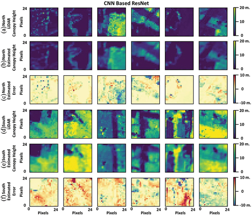
After fitting the proposed models to the northern and southern regions separately (Figure A1), the models were evaluated using the test datasets. A sample of estimated canopy height results for Seg-Net and Res-Net models is presented in Figures 4, and 5, respectively, with rows (a) and (d) presenting the LiDAR canopy heights for the northern and southern regions, respectively. Rows (b) and (e) show the estimated canopy heights using the proposed models, and finally rows (c) and (f) present the estimation error compared to the ground truth data. The figures show that the proposed models present comparable and high estimation accuracy even with the sharp variation in canopy heights, especially in the northern region. Meanwhile, the models’ results show a variation in estimation accuracy, especially in areas with narrow strips of high canopies, which can be seen in the southern region. This can be attributed to the nature of 2D-Convolution which uses an ensemble estimation window that can distort some of the pixel’s information during processing, especially when sharp changes occur in areas smaller than the size of the ensemble estimation window.

Figure 4. Canopy height estimation results using Seg-Net model for northern and southern regions, (a)(d) LiDAR observed canopy heights, (b)(e) Estimated canopy heights using the proposed model, and (c)(f) Estimation error.

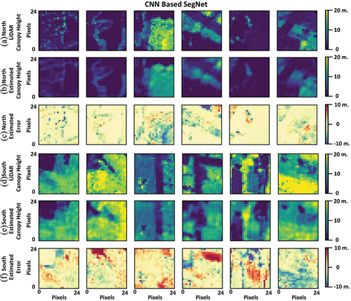
Figure 5. Canopy height estimation results using Res-Net model for northern and southern regions, (a)(d) LiDAR observed canopy heights, (b)(e) Estimated canopy heights using the proposed model, and (c)(f) Estimation error.

4.2. Performance evaluation

The fitted models are evaluated using the remaining 10% of the dataset, for the northern and southern regions separately. This is an essential step for testing the model’s generalization by using an unseen dataset to assess the model’s accuracy. The models’ performances are presented in Table 4 using MAE, RMSE, and $R^2$, and for accurate and more representative statistical analysis, an outlier threshold of $\left(2.96\sigma \right)$ was selected to filter outliers of the estimated data before statistical analysis based on random error theory (Ghilani 2017). The table shows that the average MAE and RMSE are less than 1.7 metres and 2.27 metres, respectively, for both models using the train, test, and full dataset, which demonstrate an overall high-performance accuracy for the proposed models. The performance evaluation shows variant accuracies for the same model when applied to different study regions, which is attributed to the presence of diverse canopy heights within the dataset to allow the model more versatile training. However, when evaluating the average values of the statistical parameters, we can find that both Seg-Net and Res-Net models present comparable estimation performance accuracy, with the Seg-Net model showing the highest accuracy for the full dataset evaluation with a MAE, RMSE, and coefficient of determination $\left(R^2\right)$ of 1.38 m, 1.85 m, and 0.87, respectively. These results show high estimation accuracy compared to the published literature (Table 1).

Table 4. Statistical assessment of the proposed models’ performance.

Model	Region	Train Dataset			Test Dataset			Full Dataset			Training Time (min)
		MAE (m)	RMSE (m)	$R^2$	MAE (m)	RMSE (m)	$R^2$	MAE (m)	RMSE (m)	$R^2$	(150 epochs)
Seg-Net	North	1.10	1.53	0.88	1.37	1.91	0.78	1.13	1.57	0.87	135
	South	1.59	2.08	0.88	2.02	2.64	0.82	1.63	2.14	0.87	190
	Average	1.34	1.80	0.88	1.70	2.27	0.80	1.38	1.85	0.87	162.5
Res-Net	North	1.15	1.57	0.87	1.29	1.78	0.81	1.16	1.59	0.86	690
	South	1.67	2.18	0.87	1.89	2.46	0.84	1.69	2.20	0.87	880
	Average	1.41	1.87	0.87	1.59	2.12	0.83	1.43	1.90	0.87	785

The model’s training time is highly affected by several factors, such as the size of the training dataset, the processing capacity of the training computers, the availability of GPUs, and the size of the computer’s RAM. Therefore, we used the same computer to train all the proposed models to identify and compare the required computational burden required for successful model training. It was found that the Seg-Net model converges in a much shorter time compared to the Res-Net model when using the same dataset for the same study region, (Table 4). It must be noted that the selected models’ architectures produce a very close number of trainable weights; moreover, the Seg-Net model contains more trainable weights compared to the Res-Net model. The data shows that the Seg-Net model converges 4.8 times faster than the Res-Net model on average, even with nearly the same number of trainable weights.

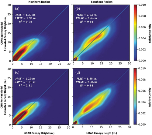
The density scatter plots for test datasets are presented in Figure 6, showing the coefficient of determination $\left(R^2\right)$ values of 0.78 and 0.81 for the northern and southern study regions, respectively, using the Seg-Net model, and 0.81 and 0.84 for the northern and southern study regions, respectively, using the Res-Net model. The presented results show that the proposed models can be used to estimate forest canopy heights with high accuracy, and a spatial resolution of 10 metres using freely available remote sensing data.

Figure 6. Density scatter plots of the LiDAR canopy heights vs the estimated canopy heights using test dataset, (a) Seg-Net for the Northern region, (b) Seg-Net for the Southern region, (c) Res-Net for the Northern region, and (d) Res-Net for Southern region.

The proposed models show different estimation accuracies for different study regions (Table 4). Therefore, the relation between the model’s MAE and canopy heights, DSM aspect, elevation, and slope are studied to evaluate their effects on the model’s performance (Figure 7).

Figure 7. Relation between (a) MAE and canopy heights, with histograms of canopy heights in the background, (b) MAE and DSM aspect, (c) MAE and DSM elevation, (d) MAE and DSM slope, (e) Canopy heights and DSM elevation, and (f) Canopy heights and DSM slope.

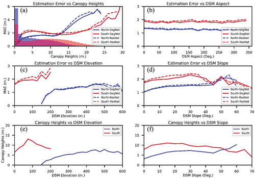
In Figure 7a, the relation between the average MAE and canopy heights is presented, in addition to the canopy height normalized histograms for both study regions. For the northern region, the models’ MAE increases proportionally with the canopy heights up to a canopy height of nearly 12 metres, then the MAE increases rapidly. This is correlated with the number of pixels available to train the model. After a canopy height of 12 m, the number of canopies in the dataset starts to decrease rapidly, which inhibits the model’s ability to learn how to estimate canopy heights higher than 12 metres. This is confirmed by the performance of the models in the southern region, with the models’ MAE starting to increase rapidly after a canopy height of 20 m because the number of canopies in the southern dataset starts to decrease after this value. Also, the MAE of the southern region is high between canopy heights of 2 to 5 metres because the number of available canopies is smaller than the number of canopies in the range of 5 to 15 metres. This is one of the downsides of ANN, the model uses the dataset to learn how to estimate the canopy heights, which is severely compromised when different values are not represented evenly in the training dataset.

In Figure 7b, the relation between the average MAE and DSM aspect is presented. It shows that there is no apparent relationship between the model MAE and the DSM aspect, which suggests that it has no effect, on its own, on the model’s accuracy. In Figure 7c, the relationship between the average MAE and DSM elevation is presented. It shows a slight incremental relationship between the MAE and DSM elevations. However, a sudden decrease in the MAE is presented between the DSM elevations of 150 to 200 metres, and it is presented in the northern dataset. Because of this observation, we present the relationship between the DSM elevation and canopy heights in Figure 7e. It demonstrates that the average canopy height decreases between elevations of 150 and 200 metres, which is the cause of the MAE decrease and is unrelated to the DSM elevation.

In Figure 7d, the relationship between the average MAE and DSM slope is presented. It shows that there is no apparent relationship between the model MAE and the DSM slope, which suggests that it has no effect, on its own, on the model’s accuracy. For confirmation, we present the relationship between the DSM slope and canopy heights in Figure 7f, which confirms that the variation in the MAE with the DSM slope is attributed to the change in average canopy heights.

In this research, we train each model separately using data from two distinct regions. A main question is whether the trained models can be used interchangeably between these two regions. As previously mentioned, we did not find a strong correlation between the trained models’ performance and the topography of the study regions. It became evident that the dataset’s representation and spread of the various canopy height values had a significant impact on the trained model’s performance. This means that if the dataset used to train the model is well balanced and represents the entire range of canopy heights expected to be in the study area, it is anticipated that the trained model will perform adequately in estimating canopy heights. By examining the datasets of our study regions (Figure 2a), we find that the southern training dataset is more dispersed and representative of a greater number of canopy height values in comparison to the training dataset of the northern region. As a result, it is expected that models trained on the southern region will perform significantly better on the northern region than models trained on the northern region when applied to the southern region. When we evaluated this hypothesis for our study regions, we found that the models trained on the northern dataset when applied to the southern region perform 1.5 times worse than the models trained on the southern dataset when applied to the northern region.

4.3. Input feature importance

This section aims at finding the influence of each input feature on the model’s accuracy using Permutation Feature Importance (Breiman 2001). The results of the models’ sensitivity analysis are illustrated in Figure 8. Several remarks can be observed from the presented sensitivity analysis, (1) the importance of a feature layer can differ between models’ architectures and study regions, mainly because each model is trained using different datasets with different structure, which yields a different estimated weight for each input feature layer. (2) The vegetation-related spectral indices present much higher importance to the model’s prediction accuracy in comparison to the Sentinel-2 observed bands. (3) DSM-related input features show low importance to the model’s prediction accuracy, which confirms the results of the model’s accuracy assessment.

Figure 8. Stem plot showing the estimated model MAE sensitivity against each input feature, (a) Seg-Net model for Northern region, (b) Seg-Net model for Southern region, (c) Res-Net model for Northern region, (d) Res-Net model for Southern region, and (c) Average estimated MAE sensitivity.

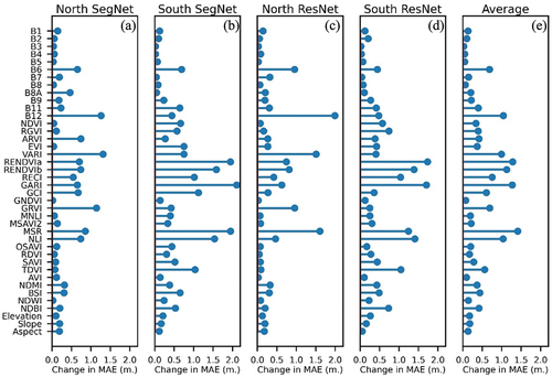
The results show that the main factor affecting the importance of the feature is the training dataset. This observation is illustrated by comparing the feature importance results of the Northern dataset in Figures 8a and c, and the Southern dataset in Figures 8b and d. The figures show that the feature importance signatures are very close when using the same dataset, even with different models’ architectures. Furthermore, with the exception of bands 6 and 12, the northern region, with its shorter canopy heights, demonstrates a high importance of some vegetation-related spectral indices over the observed Sentinel-2 data. Meanwhile, when studying the southern region, with its higher canopy heights, more vegetation related spectral indices present high importance.

The average feature importance results presented in Figure 8e demonstrate the importance of the Sentinel-2 spectral indices. The data shows that nearly all the spectral indices are significant for the canopy height estimation accuracy, with the exception of (GNDVI, AVI, and NDWI). One important observation is that only Sentinel-2 bands (6, 11, and 12) present high significance to the estimation accuracy, while bands (1, 2, 3, 4, 5, 7, and 8) show much lower significance. This demonstrates the importance of utilizing the spectral indices in canopy height estimation rather than the raw observed bands for increasing the model’s accuracy and improving conversion time.

It is evident that more input data to the ANN model increases the model’s accuracy, and if the input feature is not necessary, the ANN model will discard it by assigning low weights to it. However, processing a large amount of data regularly for monitoring purposes can be a computational challenge. Therefore, selecting the most important input features can reduce the overall running cost.

5. Conclusion

Convolution neural networks (CNNs) are one of the most influential machine learning technologies utilized in raster regression. This research presents a thorough performance evaluation of two main CNN architectures utilized in estimating forest canopy heights using remote sensing data; namely: Seg-Net and Res-Net. It also proposes deep convolution neural network variants of the two architectures characterized by their small number of trainable weights while maintaining high estimation accuracy. The proposed models were trained for canopy height estimation and evaluated using LiDAR data observed in two different regions in Thailand. To cover all the variables that may affect the accuracy of canopy height estimation, the study regions were selected to reflect variant topographic signatures, canopy height distributions, and weather conditions. The models’ performance evaluation covers the topography signature, dataset distribution, input layers, and model structure effects on the canopy height estimation accuracy and conversion time.

The analysis shows that both proposed models have high estimation accuracy, with the Encoder-Decoder CNN Seg-Net model having an advantage with an average MAE of 1.38 metres, RMSE of 1.85 metres, and $R^2$ of 0.87; it is also nearly 4.8 times faster in training conversion time than the CNN Res-Net. Moreover, the study shows that topographic characteristics such as elevation, slope, and aspect do not directly affect the model’s accuracy. However, using topographic data helps other spectral indices be more representative during model fitting and application. Weather variations in tropical regions result in variations in surface illumination, rainfall, soil moisture, cloud cover density, and surface temperature. This affects the observed surface reflectance, potentially affecting model accuracy. Furthermore, because the images used are cloud-free mosaics, it is not possible to quantify atmospheric variations to properly estimate their effect on model conversion. As a result, we tested two widely separated regions with generally different weather conditions, and it was found that proper cloud masking and atmospheric spectral corrections minimize the weather variations’ effects. Finally, the availability of diverse canopy heights in the training dataset is the main factor affecting accurate canopy height estimation. A small number of tall canopies inhibits the model from learning how to model them, which decreases its accuracy at the tallest 10% of canopies represented by the training dataset. Additionally, the importance of each input layer to the model’s estimation accuracy is evaluated and presented. It was found that Sentinel-2 spectral indices are much more important compared to the Sentinel-2 observed bands, and bands (1, 2, 3, 4, 5, 7, and 8) can be neglected.

Acknowledgements

We are grateful to the Electricity Generating Authority of Thailand (EGAT) for financing this research and providing the airborne LiDAR data, to the Japan Science and Technology Agency (JST), Kyoto University, for partially supporting this work, and to the European Space Agency for providing all the Sentinel’s remote sensing data.

Disclosure statement

No potential conflict of interest was reported by the authors.

Data availability statement

All satellite data were provided by the European Space Agency (ESA) and are publicly available via the Copernicus Open Access Hub at https://scihub.copernicus.eu/

Additional information

Funding

The work was supported by the Electricity Generating Authority of Thailand [63-I402000-21-IIR040100089000], and it was partially supported by JST-Mirai Program Grant Number JPMJMII21I3, Japan.

Appendix A

Table A1. Details of input feature layers used in the proposed ANN model.

No.	Feature Layer	Description
1	Sentinel 2 - B1	Aerosols
2	Sentinel 2 - B2	Blue
3	Sentinel 2 - B3	Green
4	Sentinel 2 - B4	Red
5	Sentinel 2 - B5	Red Edge 1
6	Sentinel 2 - B6	Red Edge 2
7	Sentinel 2 - B7	Red Edge 3
8	Sentinel 2 - B8	Near InfraRed (NIR)
9	Sentinel 2 - B8A	Red Edge 4
10	Sentinel 2 - B9	Water vapour
11	Sentinel 2 - B11	Short Wave InfraRed (SWIR) 1
12	Sentinel 2 - B12	SWIR 2
13	Normalized Difference Vegetation Index (NDVI) (Pettorelli 2013)	$\frac{\left(NIR-Red\right)}{\left(NIR+Red\right)}$
14	Red-green Vegetation Index (RGVI) (Sripada et al. 2006)	$\frac{\left(Red-Green\right)}{\left(Red+Green\right)}$
15	Atmospherically Resistant Vegetation Index (ARVI) (Kaufman and Tanre 1992)	$\frac{\left[NIR-\left(2Red-Blue\right)\right]}{\left[NIR+\left(2Red-Blue\right)\right]}$
16	Enhanced Vegetation Index (EVI) (Jiang et al. 2008)	$\frac{2.5\times \left(NIR-Red\right)}{\left(NIR+6Red-7.5Blue+1\right)}$
17	Visible Atmospherically Resistant Index (VARI) (Sun et al. 2018)	$\frac{\left(Green-Red\right)}{\left(Green+Red-Blue\right)}$
18	Red-edge Normalized Difference Vegetation Index a (RENDVIa) (Gitelson et al. 2003)	$\frac{\left(RedEdge1-Red\right)}{\left(RedEdge1+Red\right)}$
19	Red-edge Normalized Difference Vegetation Index b (RENDVIb) (Dong et al. 2019)	$\frac{\left(RedEdge2-Red\right)}{\left(RedEdge2+Red\right)}$
20	Red-edge Chlorophyll Index (RECI) (Wallis et al. 2019)	$\left(RedEdge3/RedEdge1\right)-1$
21	Green Atmospheric Resistant Index (GARI) (Gitelson, Kaufman, and Merzlyak 1996)	$\left[NIR-\left(Green-1.7\times \left(Blue-Red\right)\right)\left]/\right[NIR+\left(Green-1.7\times \left(Blue-Red\right)\right)\right]$
22	Green Chlorophyll Index (GCI) (Gitelson et al. 2003)	$\left(NIR/Green\right)-1$
23	Green Normalized Difference Vegetation Index (GNDVI) (Gitelson and Merzlyak 1998)	$\frac{\left(NIR-Green\right)}{\left(NIR+Green\right)}$
24	Green Ratio Vegetation Index (GRVI) (Sripada et al. 2006)	$\frac{NIR}{Green}$
25	Modified Non-Linear Index (MNLI) (Yang, Willis, and Mueller 2008)	$\frac{1.5\times \left(NI{R}^2-Red\right)}{\left(NI{R}^2+Red+0.5\right)}$
26	Modified Soil Adjusted Vegetation Index 2 (MSAVI2) (Qi et al. 1994)	$NIR+0.5-0.5\times \sqrt{{\left(2\times NIR+1\right)}^2-8\times \left(NIR-Red\right)}$
27	Modified Simple Ratio (MSR) (Chen 1996)	$\frac{\left(NIR/Red\right)-1}{\sqrt{NIR/Red}+1}$
28	Non-Linear Index (NLI) (Goel and Qin 1994)	$\frac{\left(NI{R}^2-Red\right)}{\left(NI{R}^2+Red\right)}$
29	Optimized Soil Adjusted Vegetation Index (OSAVI) (Rondeaux, Steven, and Baret 1996)	$\frac{\left(NIR-Red\right)}{\left(NIR+Red+0.16\right)}$
30	Renormalized Difference Vegetation Index (RDVI) (Roujean and Breon 1995)	$\frac{\left(NIR-Red\right)}{\left(\sqrt{NIR+Red}\right)}$
31	Soil Adjusted Vegetation Index (SAVI) (Huete 1988)	$\frac{1.5\times \left(NIR-Red\right)}{\left(NIR+Red+0.5\right)}$
32	Transformed Difference Vegetation Index (TDVI) (Bannari, Asalhi, and Teillet 2002)	$\frac{1.5\times \left(NIR-Red\right)}{\left(\sqrt{NI{R}^2+Red+0.5}\right)}$
33	Advanced Vegetation Index (AVI) (Roy, Sharma, and Jain 1996)	${\left[NIR\times \left(1-Red\right)\times \left(NIR-Red\right)\right]}^{1/3}$
34	Normalized Difference Moisture Index (NDMI) (Xu 2006)	$\frac{\left(NIR-SWIR1\right)}{\left(NIR+SWIR1\right)}$
35	Bare Soil Index (BSI) (Nguyen et al. 2021)	$\frac{\left(Red+SWIR1\right)-\left(NIR+Blue\right)}{\left(Red+SWIR1\right)+\left(NIR+Blue\right)}$
36	Normalized Difference Water Index (NDWI) (Gao 1996)	$\frac{\left(Green-NIR\right)}{\left(Green+NIR\right)}$
37	Normalized Difference Built-up Index (NDBI) (Zha, Gao, and Ni 2003)	$\frac{\left(SWIR1-NIR\right)}{\left(SWIR1+NIR\right)}$
38	DSM Elevation	AW3D30 DSM Elevation
39	DSM Slope	AW3D30 DSM Slope
40	DSM Aspect	AW3D30 DSM Aspect

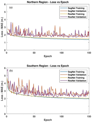
Figure A1. Loss curves for training and validation data for SegNet and ResNet models, (a) Loss curves for the Northern Region, (b) Loss curves for the Southern Region.

References

- Aamir, S., A. Shah, M. A. Manzoor, and A. Bais. 2020. “Canopy Height Estimation at Landsat Resolution Using Convolutional Neural Networks.” Machine Learning and Knowledge Extraction, February 2 (1): 23–36. doi:10.3390/make2010003.
- Alagialoglou, L., I. Manakos, M. Heurich, J. Červenka, and A. Delopoulos. 2021. “Canopy Height Estimation from Spaceborne Imagery Using Convolutional Encoder-Decoder.“ In MultiMedia Modeling: 27th International Conference, MMM 2021, Prague, Czech Republic, June 22–24, 2021, Proceedings, Part II 27, pp. 307–317. Springer International Publishing
- Bannari, A., H. Asalhi, and P. M. Teillet. 2002. Transformed Difference Vegetation Index (TDVI) for Vegetation Cover Mapping. International Geoscience and Remote Sensing Symposium (IGARSS), 24-28 June 2002, Toronto, ON, Canada, Volume 5, pp. 3053–3055. doi:10.1109/IGARSS.2002.1026867.
- Bisong, E., 2019. Google Colaboratory. Building Machine Learning and Deep Learning Models on Google Cloud Platform, pp. 59–64.
- Breiman, L. 2001. “Random Forests.” Machine Learning 45 (1, October): 5–32. doi:10.1023/A:1010933404324.
- Chen, J. M. 1996. “Evaluation of Vegetation Indices and a Modified Simple Ratio for Boreal Applications.” Canadian Journal of Remote Sensing 22 (3): 229–242. doi:10.1080/07038992.1996.10855178.
- Cloude, S. R., and K. Papathanassiou, 1998. Polarimetric SAR Interferometry. IEEE Transactions on geoscience and remote sensing 36 (5): 1551–1565. doi:10.1109/36.718859.
- Cloude, S. R., and K. P. Papathanassiou. 2003. “Three-Stage Inversion Process for Polarimetric SAR Interferometry.” IEE Proceedings: Radar, Sonar and Navigation 150 (3, June): 125–134. doi:10.1049/ip-rsn:20030449.
- Dong, T., J. Liu, J. Shang, B. Qian, B. Ma, J. M. Kovacs, D. Walters, X. Jiao, X. Geng, and Y. Shi. 2019. “Assessment of Red-Edge Vegetation Indices for Crop Leaf Area Index Estimation.” Remote Sensing of Environment 222 (March): 133–143. doi:10.1016/j.rse.2018.12.032.
- Gale, M. G., G. J. Cary, A. I. Van Dijk, and M. Yebra. 2021. “Forest Fire Fuel Through the Lens of Remote Sensing: Review of Approaches, Challenges and Future Directions in the Remote Sensing of Biotic Determinants of Fire Behaviour.” Remote Sensing of Environment 255: 112282. doi:10.1016/j.rse.2020.112282.
- Gao, B. C. 1996. “Ndwi—a Normalized Difference Water Index for Remote Sensing of Vegetation Liquid Water from Space.” Remote Sensing of Environment 58 (3, December): 257–266. doi:10.1016/S0034-4257(96)00067-3.
- Ghilani, C. D. 2017. Adjustment Computations: Spatial Data Analysis. Hoboken, New Jersey, USA: John Wiley & Sons.
- Gholz, H. L., K. Nakane, and H. Shimoda. 2012. The Use of Remote Sensing in the Modeling of Forest Productivity. s.l: Springer Science & Business Media.
- Gitelson, A. A., Y. J. Kaufman, and M. N. Merzlyak. 1996. “Use of a Green Channel in Remote Sensing of Global Vegetation from EOS-MODIS.” Remote Sensing of Environment 58 (3, December): 289–298. doi:10.1016/S0034-4257(96)00072-7.
- Gitelson, A. A., and M. N. Merzlyak. 1998. “Remote Sensing of Chlorophyll Concentration in Higher Plant Leaves.” Advances in Space Research 22 (5, January): 689–692. doi:10.1016/S0273-1177(97)01133-2.
- Gitelson, A. A., A. Viña, T. J. Arkebauer, D. C. Rundquist, G. Keydan, and B. Leavitt. 2003. “Remote Estimation of Leaf Area Index and Green Leaf Biomass in Maize Canopies.” Geophysical Research Letters 30 (5, March). doi:10.1029/2002GL016450.
- Goel, N. S., and W. Qin. 1994. “Influences of Canopy Architecture on Relationships Between Various Vegetation Indices and LAI and FPAR: A Computer Simulation.” Remote Sensing Reviews 10 (4): 309–347. doi:10.1080/02757259409532252.
- Gorelick, N., M. Hancher, M. Dixon, S. Ilyushchenko, D. Thau, and R. Moore. 2017. “Google Earth Engine: Planetary-Scale Geospatial Analysis for Everyone.” Remote Sensing of Environment 202 (December): 18–27. doi:10.1016/j.rse.2017.06.031.
- Hansen, M. C., P. V. Potapov, S. J. Goetz, S. Turubanova, A. Tyukavina, A. Krylov, A. Kommareddy, and A. Egorov. 2016. “Mapping Tree Height Distributions in Sub-Saharan Africa Using Landsat 7 and 8 Data.” Remote Sensing of Environment 185 (November): 221–232. doi:10.1016/j.rse.2016.02.023.
- Huete, A. R. 1988. “A Soil-Adjusted Vegetation Index (SAVI).” Remote Sensing of Environment 25 (3, August): 295–309. doi:10.1016/0034-4257(88)90106-X.
- Jiang, Z., A. R. Huete, K. Didan, and T. Miura. 2008. “Development of a Two-Band Enhanced Vegetation Index Without a Blue Band.” Remote Sensing of Environment 112 (10): 3833–3845. doi:10.1016/j.rse.2008.06.006.
- Kaufman, Y. J., and D. Tanre. 1992. “Atmospherically Resistant Vegetation Index (ARVI) for EOS-MODIS.” IEEE Transactions on Geoscience and Remote Sensing 30 (2): 261–270. doi:10.1109/36.134076.
- Kingma, D. P., and J. Ba. 2014. “Adam: A Method for Stochastic Optimization.” arXiv preprint arXiv:1412.6980 December. https://arxiv.org/abs/1412.6980
- Kugler, F., S. K. Lee, I. Hajnsek, and K. P. Papathanassiou. 2015. “Forest Height Estimation by Means of Pol-InSar Data Inversion: The Role of the Vertical Wavenumber.” IEEE Transactions on Geoscience and Remote Sensing 53 (10, October): 5294–5311. doi:10.1109/TGRS.2015.2420996.
- Lang, N., K. Schindler, and J. D. Wegner. 2019. “Country-Wide High-Resolution Vegetation Height Mapping with Sentinel-2.” Remote Sensing of Environment 233 (November): 111347. doi:10.1016/j.rse.2019.111347.
- Lavalle, M., M. Simard, and S. Hensley. 2011. “A Temporal Decorrelation Model for Polarimetric Radar Interferometers.” IEEE Transactions on Geoscience and Remote Sensing 50 (7): 2880–2888. doi:10.1109/TGRS.2011.2174367.
- Li, W., Z. Niu, R. Shang, Y. Qin, L. Wang, and H. Chen. 2020. “High-Resolution Mapping of Forest Canopy Height Using Machine Learning by Coupling ICESat-2 LiDar with Sentinel-1, Sentinel-2 and Landsat-8 Data.” International Journal of Applied Earth Observation and Geoinformation 92 (October): 102163. doi:10.1016/j.jag.2020.102163.
- Liu, X., Y. Su, T. Hu, Q. Yang, B. Liu, Y. Deng, H. Tang, Z. Tang, J. Fang, and Q. Guo. 2022. “Neural Network Guided Interpolation for Mapping Canopy Height of China’s Forests by Integrating GEDI and ICESat-2 Data.” Remote Sensing of Environment 269: 112844. doi:10.1016/j.rse.2021.112844.
- Main-Knorn, M., B. Pflug, J. Louis, V. Debaecker, U. Müller-Wilm, and F. Gascon. 2017. “Sen2Cor for sentinel-2.” In Image and Signal Processing for Remote Sensing XXIII 2017 Oct 4, 10427, 37–48. Warsaw, Poland: Society of Photo-Optical Instrumentation Engineers (SPIE). doi:10.1117/12.2278218.
- Myeong, S., D. J. Nowak, and M. J. Duggin. 2006. “A Temporal Analysis of Urban Forest Carbon Storage Using Remote Sensing.” Remote Sensing of Environment 101 (2): 277–282. doi:10.1016/j.rse.2005.12.001.
- Nguyen, C. T., A. Chidthaisong, P. Kieu Diem, and L. -Z. Huo. 2021. “A Modified Bare Soil Index to Identify Bare Land Features During Agricultural Fallow-Period in Southeast Asia Using Landsat 8.” Land 10 (3, February): 231. doi:10.3390/land10030231.
- Papathanassiou, K. P., and S. Cloude. 2001. “Single-Baseline Polarimetric SAR Interferometry.” IEEE Transactions on Geoscience and Remote Sensing 39 (11): 2352–2363. doi:10.1109/36.964971.
- Pettorelli, N. 2013. The Normalized Difference Vegetation Index. s.l: Oxford University Press.
- Qi, J., A. Chehbouni, A. R. Huete, Y. H. Kerr, and S. Sorooshian. 1994. “A Modified Soil Adjusted Vegetation Index.” Remote Sensing of Environment 48 (2, May): 119–126. doi:10.1016/0034-4257(94)90134-1.
- Rondeaux, G., M. Steven, and F. Baret. 1996. “Optimization of Soil-Adjusted Vegetation Indices.” Remote Sensing of Environment 55 (2, February): 95–107. doi:10.1016/0034-4257(95)00186-7.
- Roujean, J. L., and F. M. Breon. 1995. “Estimating PAR Absorbed by Vegetation from Bidirectional Reflectance Measurements.” Remote Sensing of Environment 51 (3, March): 375–384. doi:10.1016/0034-4257(94)00114-3.
- Roy, P., K. Sharma, and A. Jain. 1996. “Stratification of Density in Dry Deciduous Forest Using Satellite Remote Sensing Digital Data—an Approach Based on Spectral Indices.” Journal of Biosciences 21 (5): 723–734. doi:10.1007/BF02703148.
- Sripada, R. P., R. W. Heiniger, J. G. White, and A. D. Meijer. 2006. “Aerial Color Infrared Photography for Determining Early In-Season Nitrogen Requirements in Corn.” Agronomy Journal 98 (4, July): 968–977. doi:10.2134/agronj2005.0200.
- Sun, H., Q. Wang, G. Wang, H. Lin, P. Luo, J. Li, S. Zeng, X. Xu, and L. Ren. 2018. “Optimizing kNn for Mapping Vegetation Cover of Arid and Semi-Arid Areas Using Landsat Images.” Remote Sensing 10 (8, August): 1248. doi:10.3390/rs10081248.
- Takaku, J., T. Tadono, and K. Tsutsui. 2014. “GENERATION OF HIGH RESOLUTION GLOBAL DSM FROM ALOS PRISM.” ISPRS Annals of Photogrammetry, Remote Sensing & Spatial Information Sciences 4 (2): 243–248. doi:10.5194/isprsarchives-XL-4-243-2014.
- Wallis, C. I. B., J. Homeier, J. Peña, R. Brandl, N. Farwig, and J. Bendix. 2019. “Modeling Tropical Montane Forest Biomass, Productivity and Canopy Traits with Multispectral Remote Sensing Data.” Remote Sensing of Environment 225 (May): 77–92. doi:10.1016/j.rse.2019.02.021.
- Wenxue, F., G. Huadong, L. Xinwu, T. Bangsen, and S. Zhongchang. 2015. “Extended Three-Stage Polarimetric SAR Interferometry Algorithm by Dual-Polarization Data.” IEEE Transactions on Geoscience and Remote Sensing 54 (5, May): 2792–2802. doi:10.1109/TGRS.2015.2505707.
- Xu, H. 2006. “Modification of Normalised Difference Water Index (NDWI) to Enhance Open Water Features in Remotely Sensed Imagery.” International Journal of Remote Sensing 27 (14, July): 3025–3033. doi:10.1080/01431160600589179.
- Yang, Z., P. Willis, and R. Mueller. 2008. “Impact of Band-Ratio Enhanced AWIFS Image to Crop Classification Accuracy.” Proceeding Pecora 17 (1): 1–11.
- Zha, Y., J. Gao, and S. Ni. 2003. “Use of Normalized Difference Built-Up Index in Automatically Mapping Urban Areas from TM Imagery.” International Journal of Remote Sensing 24 (3): 583–594. doi:10.1080/01431160304987.
- Zhao, K., S. Popescu, and R. Nelson. 2009. “Lidar Remote Sensing of Forest Biomass: A Scale-Invariant Estimation Approach Using Airborne Lasers.” Remote Sensing of Environment 113 (1): 182–196. doi:10.1016/j.rse.2008.09.009.
- Zhao, Y., Y. Zeng, Z. Zheng, W. Dong, D. Zhao, B. Wu, and Q. Zhao. 2018. “Forest Species Diversity Mapping Using Airborne LiDar and Hyperspectral Data in a Subtropical Forest in China.” Remote Sensing of Environment 213: 104–114. doi:10.1016/j.rse.2018.05.014.