The effect of altitude on the uncertainty of radar-based precipitation estimates over Switzerland

ABSTRACT

Despite high spatial coverage, radar-based Quantitative Precipitation Estimates (QPE) are affected by different sources of errors. Regardless of various techniques to merge these estimates with rain gauges, some errors still remain in the final product. This study focused on the relationship between these errors and altitude for a radar-only product (RZC) and a cross-validated-merged-with-gauge product (CPC-CV) in Switzerland using 16 years of hourly data based on two log-transformed metrics (bias and scatter). For each site, the bias is a measure of the mean error and the scatter is a robust estimate of the dispersion of the error around the mean. The results showed that the bias has a negative Pearson correlation coefficient with altitude, while the scatter has a positive correlation for both RZC and CPC-CV products during the entire period. Considering the effect of the old and the new networks, the errors are generally reduced using the new radar network. However, the relationship between altitude and the errors is still present. Regarding the seasonality effect, the results showed a significant underestimation at low altitudes and the weakest bias correlation in winter, while many stations showed overestimation in summer. For scatter, the correlation with altitude was highest in summer, while it was low in winter. Moreover, for low-intensity precipitation (below 1.1 $\mathit{mm}.h^{-1}$) there is a negative correlation for bias and a positive correlation for scatter with the gauge altitudes in both products. Interestingly, for high intensities (above 7 $\mathit{mm}.h^{-1}$), a positive correlation for bias and a negative correlation for scatter was observed . Also, we added the bias of eight glaciers based on the snow depth measurements in addition to the gauge data. In conclusion, the results showed that almost 30% of the variance of the errors in both products can be statistically explained using the gauge altitudes as a single explanatory variable.

KEYWORDS:

• Precipitation measurement
• Quantitative Precipitation Estimates
• Altitudinal effect

1. Introduction

It is generally accepted that altitude plays an essential role in the spatial distribution of precipitation in mountainous areas due to the decrease in temperature and the increase in condensation with altitude (Sevruk 1997). However, having robust observational precipitation data in those areas is challenging. Since precipitation characteristics change rapidly in time and space and gauge networks are often not dense enough, estimates of gauge networks may suffer from representativeness errors in most areas (Sokol and Bližňák 2009). This issue is more pronounced in steep valleys and high-altitude mountains due to the complications of installing and operating dense networks in such areas. This results in an unbalanced distribution of the gauges among valley floors and mountains, which may introduce systematic errors for gauge-based products.

Although radar precipitation estimates can provide data with high spatial coverage in a fine temporal resolution, they are affected by different sources of errors, for instance: ground clutter, bright band effect, and the uncertainty around the empirical transformation of reflectivity to rain rate. A detailed review of the errors and uncertainties in radar estimates can be found in Berne and Krajewski (2013). In mountainous areas, some errors such as beam shielding, ground clutter, and errors due to more frequent snowfalls (which have more difficulties in characterizing the scattering properties of the snowflakes) are expected to increase (Germann et al. 2006).

Various techniques have been applied for merging radar estimates with gauge measurements in order to reduce the uncertainties of precipitation estimates, such as Krajewski (1987); Seo and Breidenbach (2002); Gabella and Notarpietro (2004); Haiden et al. (2011). However, the aforementioned weaknesses in each gauge measurements and radar estimates still affect the final product. These uncertainties in final merged gauge-radar products, which are due to remaining uncorrected errors, processing errors, and approximations (Cecinati et al. 2017), are considered as residual errors.

There are numerous studies regarding gauge-radar estimates and their errors in the Alpine region, e.g. Germann et al. (2006); Sideris et al. (2014); Kann et al. (2015); Panziera et al. (2018); Le Bastard et al. (2019). In addition, the effect of altitude on precipitation in the Alpine areas has been separately analysed in several studies, such as: Sevruk (1997); Faure, Delrieu, and Gaussiat (2019); Grünewald and Lehning (2011). Faure, Delrieu, and Gaussiat (2019) studied the relative altitudinal gradient of precipitation estimates for three massifs in the French Alps in 2016. They used 23 gauges located in different altitudes from 220 m above mean sea level (m.s.l) to 1730 m.s.l, as well as a merged Quantitative Precipitation Estimates (QPE) product based on 29 radars for the year 2016. The results suggest that the QPE tends to overestimate precipitation in lower altitudes and underestimates at higher altitudes. They concluded that it is difficult to estimate the altitudinal gradient of precipitation at the daily timescale, probably due to the limited number of gauges in higher altitudes (Faure, Delrieu, and Gaussiat 2019).

In Switzerland, Servuk (1997) studied the regional dependencies of precipitation and altitude using gauge measurements. The results highlighted the noticeable difference in precipitation-altitude dependency between the northern and southern Alps divided by the main Alpine ridge. In general, precipitation in the northern parts of the Alps showed a stronger dependency on the altitude compared to the southern parts (Sevruk 1997).

To reduce the bias of the radar estimates, Gabella, Joss, and Perona (2000) proposed a weighted multiple regression approach based on three independent variables: a) the distance between radar and gauge, b) the height of visibility, and c) the altitude of the gauge site. The altitude of the gauge site was implemented to indicate the depth of the growth layer related to the topography (Gabella, Joss, and Perona 2000). This study was followed by Gabella and Notarpietro (2004), where the weighted regression was employed to explain the variability of gauge-radar. Based on four events over the northern Italian Alps, the results showed that the distance from radar and radar visibility significantly affect the variability of the radar-gauge bias. These two parameters are negatively correlated with the bias, i.e. the radar underestimates precipitation in higher sampling volumes and longer distances. Based on this study, the uncertainty of the altitudinal effect is larger, and it can be positive or negative.

Although the precipitation–altitude relationship using gauge measurements has been subjected to many studies, the effect of altitude on radar residual errors is still not very well understood. This is partly due to the difficulties of assessing the systematic effect of altitude on precipitation, where long-term data are essential to study the precipitation–altitude relationship (Masson and Frei 2014). To deal with this challenge, we use 16 years of hourly precipitation data to study the effect of altitude on radar residual errors over Switzerland. The Swiss radar network was based on three single polarization radars named Albis, La Dole, and Monte Lema (Germann et al. 2006) and has been upgraded to dual-polarization radars in 2011 (La Dole and Monte Lema) and in 2012 (Albis). Two new dual-polarization radars (Plaine Morte and Weissfluhgipfel) were installed in 2013 and 2015 and have been operational since 2014 and 2016. More details about the new radar network can be found in Gabella et al. (2017) and Germann et al. (2022).

By implementing an empirical statistical approach, we analyse this effect on the old and new networks, seasons, and the role of precipitation intensity. Unlike the aforementioned studies, we focus on the altitudinal dependency of the errors in two QPE products using long-term hourly data of 279 stations over the entire Switzerland. The following questions are addressed in this study:

(1) What is the relationship between radar residual errors and the gauge altitudes over Switzerland?

(2) What are the possible explanations for the relationship between the errors and altitude over Switzerland?

(3) How do changes in radar networks, seasonality, and intensity, affect this relationship?

This paper is structured as follows: Section 2 describes the datasets and methodology. The results are presented in section 3 and discussed in section 4. In section 5 the conclusions of this study are drawn.

2. Materials and methods

2.1. Study area and dataset

Figure 1 shows the study area (entire Switzerland), the spatial distribution of the stations, and the locations of the radars in the country. The letters indicate the name of the radars, i.e. Albis (A), La Dole (D), Monte Lema (L), Plaine Morte (P), and Weissfluhgipfel (W). The Alpine mountains, as well as the Jura mountains in the northwest, mainly characterize the geography of Switzerland. From geographical and climatological perspectives, the study domain can be divided into four different sub-regions: the northwest (Jura mountains), the northeast, the Alpine mountains, and the southern Alps (Molnar and Burlando 2008). While the northwest is separated from the northeast by the wet anomaly of the Jura mountains, the south region around Lake Maggiore is mainly influenced by Mediterranean cyclonic activity during autumn. The mean annual and seasonal precipitation do not vary significantly between the regions, except for the southern part, where convective storms lead to more precipitation in the summer and autumn seasons than in the rest of the year. In the Alpine region, summer is the main rainy season (Frei and Schär 1998).

Figure 1. Spatial distribution of the gauges and the locations of five radars (left), and a histogram of the station altitudes (right) over Switzerland. Note that the map extends from 5.53^° E and 45.46^° N (bottom left) to 10.38^° E to 47.48^° N (top right) in World Geodetic System (WGS84).

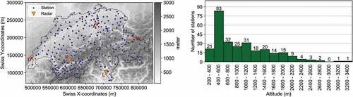
We use 16 years (2005–2021) of hourly aggregated data generated from measurements of 279 rain-gauges of the Swiss national rain-gauge network. The minimum and maximum altitudes of the locations of these stations are 203 m and 3302 m, respectively, with an average of 998 m above sea level. It is worth mentioning that the lowest point in Switzerland is 193 m above sea level (at lake Maggiore). Note that not all of these 279 stations have been operational for the entire aforementioned 16-year period. New stations have been progressively added to the network (especially after 2009), while a few old ones have been decommissioned. Rain-gauge measurements, as well as other meteorological variables, are subject to extensive MeteoSwiss internal quality control (Grüter et al. 2003). In short, the internal quality control algorithm involves the following tests: a) Limit tests (comparison with physical and climatological limits), b) Variability tests (tests of maximum and minimum acceptable variability during a specified time interval), c) Inter-parameter consistency tests (values of variables measured at the same time and place cannot be inconsistent with each other), d) Spatial consistency tests (between nearby stations). This is basically a gauge-kriging algorithm using altitude as an external drift (see Schwarb 2000), the so-called ‘PRISM’ algorithm).

Several QPE products are in use in Switzerland. Besides the standard radar-only product (hereafter RZC), Sideris et al. (2014) introduced a co-kriging-based technique to generate a merged radar-rain gauge product named CombiPrecip (hereafter CPC). Panziera et al. (2018) used the cross-validation (leave-one-out) output of CPC (hereafter CPC-CV) in their study. Recently, a new product has been developed which exploits the capabilities of the newly installed dual-polarization radar data and uses a random forest algorithm (Wolfensberger et al. 2021).

We use hourly aggregated data of the gauges and the two radar-based products (RZC and CPC-CV) from December 2004 to August 2021, excluding the year 2011. This is because 2011 was the year of the installation of two new-generation Swiss radars, and the radar estimates have rendered some problems which may affect the reliability of the radar estimates during this year. Based on changes in the radar network and the number of stations, the data can be divided into three sub-periods.

Period 1: From December 2004 to the end of 2010, the network included 3 single-polarization radars, while the number of stations increased from 72 in 2005 to 89 by the end of 2010.

Period 2: From 2012 to the end of 2015, two dual-polarization radars were installed as well as the upgrading of the three existing ones to dual-polarization radars took place. In addition, the number of stations increased to 261 during this period. We use the data from period 2 only in our overall analyses and exclude them for the rest of the study because of the significant changes in radar and gauge networks during that period.

Period 3: From the beginning of 2016 until August 2021 (the last period), 15 more stations were added to the network.

In conjunction with RZC product, we use the cross-validated output (CPC-CV) to ensure that the gauge observations have not been used for the merging algorithm.

2.2. Methodology

The residual errors of a radar product are usually characterized by two components: systematic error and random error (Ciach, Krajewski, and Villarini 2007). Due to the dominance of the multiplicative nature of the systematic error compared to the additive one (Gabella et al. 2017; Germann et al. 2009), we define bias as the representative of the mean error as below:

(1) $\mathit{bias}=10\mathit{lo}{g}_{10}(R_r/R_g)$(1)

where $R_r$ is the accumulated radar estimates over time at the gauge location, $R_g$ is the accumulated gauge measurements over time as the approximation of true precipitation. Note that the accumulated radar estimates are derived from the pixel that each gauge is located, making the method pixel (1 km radar grid) to point (gauge) comparison. The advantage of having a log-transformed bias is that we have an almost Gaussian distribution of the error (Cecinati et al. 2017). To calculate the bias component, there are three approaches: unconditional (including wet and dry hours), single-conditional bias (based on wet hours of the reference), and double-conditional bias (only wet hours in both gauge and radar estimates). In this study, we use a single-conditional bias approach, which means to set a minimum threshold for the gauge measurements (as the reference estimates), but considering all values for the radar estimates (without any threshold). Here we set the value 0.3 $\mathit{mm}.h^{-1}$ as the minimum intensity threshold measured as the gauge resolution. We use the scatter metric to show the dispersion of the gauge-radar error around the mean, available in Pysteps package (Pulkkinen et al. 2019), which is defined as the half distance between 16% and 84% of the cumulative distribution of total precipitation as a function of gauge-radar ratio (in dB) (Germann et al. 2004).

Note that the bias is a measure of the mean error and represents the overall adjustment multiplicative factor that one should apply to make the total radar estimates coincident with the gauge amount at the gauge location. The scatter, here is calculated based on hourly rain rates, is a robust estimate of the dispersion of the error around the mean and it is perfectly orthogonal to the bias. Any multiplicative factor applied to radar (or gauge) amounts has no influence on the scatter (Gabella et al. 2017).

As a common and simple approach to modelling the precipitation-altitude relationship (Masson and Frei 2014), we use a linear regression (Equation 2(2) $\mathit{y}=\mathit{\alpha x}+\mathit{\beta }$(2) ) to demonstrate the relationship between radar residual errors and the gauge altitudes. Note that although the regression equation is linear, the bias and scatter parameters, as the dependent variables, are log-transformed. Using these log-transformed variables makes the relationship non-linear, and it is a common approach where a non-linear relationship exists (Benoit 2011). We use the gauge altitudes as the predictor for radar residual errors as follows:

(2) $\mathit{y}=\mathit{\alpha x}+\mathit{\beta }$(2)

where $\mathit{y}$ is a component of radar residual errors (bias or scatter) in the two radar products (RZC and CPC-CV) and$\mathit{x}$ is the normalized altitude. The normalized altitude for each station is defined as follows:

(3) $\mathit{x}=\frac{(x_0-x_n)}{x_n}$(3)

where$x_0$ is the altitude of each station (in metre),$\mathit{x}$ is the normalized altitude, and$x_n$ is the normalization altitude (1000 m). Note that the average altitude for the stations in Switzerland is 998 m, which we round to 1000 m as the normalization altitude. The advantage of using centred and normalized altitudes is more esthetical so that the parameters in Equation 2(2) $\mathit{y}=\mathit{\alpha x}+\mathit{\beta }$(2) become more interpretable. Using centred values, the intercept ($\mathit{\beta }$) in Equation 2(2) $\mathit{y}=\mathit{\alpha x}+\mathit{\beta }$(2) represents the residual error in dB at the average gauge altitude, while the normalization ensures that the slope ($\mathit{\alpha }$) remains in a range around $\pm 1$. Finally, the normalization produces a dimensionless quantity that can be log-transformed following Gabella et al. (2005) approach. In order to determine the correlation between radar residual errors and the gauge altitudes, the Pearson correlation coefficient (hereafter CC) for each error component (e) is calculated as below:

(4) $\mathit{CC}=\frac{{\sum }_{i=1}^n(x_i-\bar{x})(e_i-\bar{e})}{\sqrt{{\sum }_{i=1}^n{(x_i-\bar{x})}^2}\sqrt{{\sum }_{i=1}^n{(e_i-\bar{e})}^2}}$(4)

where$x_i$ is the normalized altitude of the station$\mathit{i}$, $\bar{x}$ is the mean of the normalized altitudes of the stations,$e_i$ is the error component (bias or scatter) in each station, and $\bar{e}$ is the mean of the error component for all the stations.

To investigate the possible changes in the relationship between residual errors and altitude in different seasons, we employ a regression for each season, i.e. winter (December to February), spring (March to April), summer (June to August), and autumn (September to November). Note that we only consider the last period (2016–2021) for this section to eliminate the effect of using different subsets of gauges and different radar networks in our analysis. For each season, we calculate bias and scatter and derive the regression parameters for each station.

Furthermore, we study the possible effect of intensity on the error–altitude relationship using the data from period 3 (2016 to 2021). First, we define low and high precipitation intensity thresholds and then we include all the events below for low threshold and above for high threshold intensities. The low threshold is set as 1.1 $\mathit{mm}.h^{-1}$, and the high threshold as 7 $\mathit{mm}.h^{-1}$, values that correspond to the 60th and the 98.5th percentiles, respectively. Note that these values are based on the precipitation intensity measured by the gauges and are chosen empirically based on the authors’ experience regarding precipitation intensity in Switzerland. The fact that the number of events with more than the high-intensity threshold is limited might have some negative effects on the interpretation of the results. Hence, we calculate bias and scatter for any number of events ($\mathit{n}>=1$), but also conditionally: the minimum number of events should be greater than 10 at each gauge ($\mathit{n}>10$). Using one threshold for high (and one for low) intensities can provide valuable information about the tails of the intensity distribution, which can be useful for impact-based hydrological studies. In order to include all parts of the distribution and the interaction between the estimates of radar and gauge intensities, we use a multi-threshold approach based on the intensities in both gauges and radar. Hence, we define 25 categories based on different intensities estimated by both gauge and radar, and calculate the correlation for each category.

3. Results

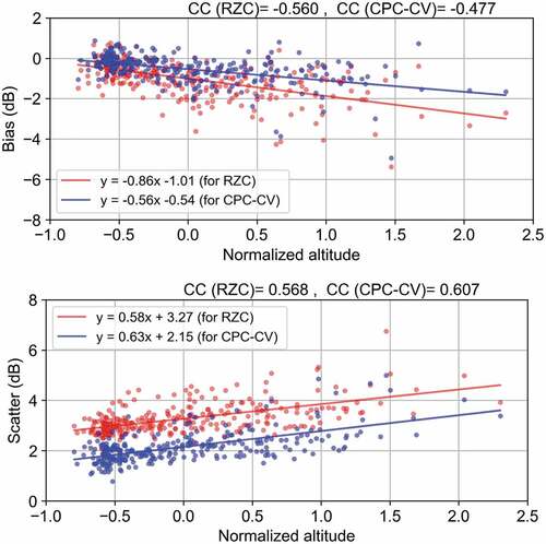
As a first step, bias and scatter are calculated using the accumulated precipitation of the gauges and the two radar products for the entire 16-year period. Figure 2 shows bias and scatter as a function of the normalized gauge altitudes for the two products. The parameters of the regression model for all 16 years as well as for the last six years (period 3) are computed and summarized in Tables 4 and 5 in Appendix A. Based on these results, the bias has a negative trend with altitude, while the scatter shows a positive trend. In addition, the uncertainty of the slope is approximately the same in all the regressions: it is of the order of 0.06–0.08 for bias and 0.04–0.05 for the scatter. As expected, CPC-CV shows smaller residual errors, and compared to RZC, the regression model for CPC-CV bias shows a milder slope with a slightly lower correlation. For scatter, CPC-CV shows a decrease at the intercept altitude at 1 km by more than 1 dB. The slope and correlation, nevertheless, showed similar values, even slightly more than RZC.

Figure 2. Total bias (top) and scatter (bottom) from 2005 to 2021 as a function of the normalized gauge altitudes for RZC (red) and CPC-CV (blue). Note that the normalized altitudes of −1, −.5, 0, and 0.5 correspond to actual altitudes of 0, 0.5, 1, and 1.5 km, respectively.

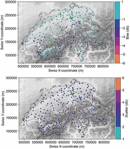
The presence of five (instead of three) radars and 277 stations during period 3 (2016–2021) helped to improve the radar estimates. In this period, the regression model performs reasonably well with a correlation of −0.50 and 0.45 for bias and scatter of RZC product, respectively (Tables A1 and A2 in Appendix A). Figure 3 shows a spatial distribution of bias and scatter for the RZC product during period 3 (2016–2021). Despite positive biases for a few stations over the northern part of the Alps, RZC underestimates precipitation in most of the stations over Switzerland. During period 3, the altitudinal dependency of the CPC-CV bias is similar to that of the RZC product with a milder gradient. It is worth mentioning that using the CPC-CV product noticeably improved the bias in the Alpine ridge (Figure A1 in Appendix A).

Figure 3. Spatial distribution of total bias (top) and scatter (bottom) for RZC from 2016 to 2021. Note that the yellow triangular symbols show the location of the radars and the map extends from 5.53^° E and 45.46^° N (bottom left) to 10.38 E to 47.48 N (top right) in World Geodetic System (WGS84).

In general, changes in the radar network and adding new stations reduced the residual errors. Moreover, both bias and scatter -as two multiplicative representatives of the residual errors- show a clear dependency on the gauges’ altitudes.

3.1. The effect of the new radar network

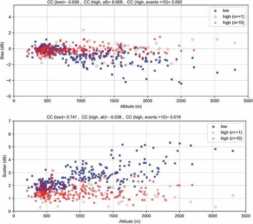
In order to analyse the effect of upgrading the radar network from three (2005–2011) to five radars (2016–2021), we employ the measurements of the 72 stations that were operational and provided measurements in both of these periods. Figure 4 shows how the RZC bias (top) and the scatter (bottom) change with altitude for the old and new radar networks based on these 72 stations. The bias for the new radar network decreases in many stations and shows a better correlation with the altitude of the gauges. In the 2016–2021 period, many stations mostly underestimated precipitation despite having positive biases during the first period. For scatter, the altitudinal dependency has decreased using the new radar network. It is worth mentioning that the uncertainty of the slope for both bias and scatter has decreased in the new radar network (Tables A3 and A4 Appendix A).

Figure 4. Total bias (top) and scatter (bottom) for the old and the new radar networks based on the 72 gauges that measured precipitation in both networks as a function of the gauge altitudes.

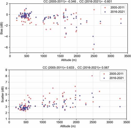
The results for CPC-CV products show similar behaviours as RZC in terms of bias for both periods. For scatter, despite the decrease of the errors in each station in the last period, its correlation to the gauge altitudes remains similar to the first period (not shown). The regression parameters for different networks are summarized in Tables A3 and A4 Appendix A. In most stations, the new radar network was able to reduce residual errors, especially in mountainous areas. This is due to the presence of two newly installed radars (Pointe de la Plaine Morte and Weissfluhgipfel) which improved the network visibility in the inner Alpine regions. This effect is more pronounced for the stations close to the Weissfluhgipfel radar (Figure A2 Appendix A). For instance, at the two highest gauges located in the mountainous region Grisons, the bias error was reduced up to 2 dB for the station Weissfluhjoch (WFJ, using MeteoSwiss nomenclature, 2691 m) while for the station Corvatsch (COV, 3300 m) the scatter was improved by more than 1 dB. Installation of the two new radars has a clear positive effect in reducing the scatter in most stations over the country. Note that the −6 dB Bias at the”Colle del Gran San Bernardo” (GSB, altitude 2472 m) is also caused by several false precipitation amounts affecting the gauge values, such as fresh snow blown by the wind into the gauge. This is reflected in the substantial value of the scatter, which reaches the almost unbelievable value of 7 dB. Data from a new, better site (less prone to false precipitation) have been available since the beginning of February 2020, which has improved the situation. This can be partly observed in Figure 4, where the GSB red dot (6-year period up to 2010) shows a scatter of 8 dB, while the blue dot (6-year period, of which 2020 and 2021 at the new site) shows a scatter of 5 dB.

3.2. The seasonality effect

Figure 5 shows the relationship between bias and scatter with the gauges’ altitude in four seasons. By checking the intercept values in Table 1, the predicted bias at the median altitude of 1 km shows the largest radar underestimation during winter (1.57 dB). In general, bias shows a large radar underestimation during winter in low altitudes, which causes a weak bias correlation (−0.2) and mild slope (−0.41) with altitude. During autumn and spring, the correlation and the slope show noticeably higher values than in winter and summer (Table 1). During summer, the bias shows the lowest predicted value at the median altitude of 1 km (−0.03 dB) when almost half of the stations (mostly located below 1500 m) overestimate precipitation. The uncertainty of the slope for bias is smaller in summer (0.06) compared to the other 3 seasons (0.10–0.12). As far as the scatter is concerned Table 2, the predicted scatter at the median altitude of 1 km is the lowest in summer (2.81 dB) and the second largest in winter (3.13 dB). The results show smaller scatter values in low altitudes in summer. The increase of scatter with altitude shows the largest correlation in summer: the explained variance is of the order of 25%. In the other three seasons, the range is from 7% (spring) to 15% (autumn). The uncertainty of the slope is approximately the same in all 4 seasons for scatter (0.04–0.05), which is just like for the whole year. In addition, the results for CPC-CV show that bias and scatter decrease noticeably in lower altitudes, especially in the autumn and winter seasons (Figure A3 Appendix A). A higher correlation for CPC-CV indicates that CPC-CV clearly reduces the errors at lower altitudes, especially in winter, but its performance slightly decreases at higher altitudes.

Figure 5. Total RZC bias (top) and scatter (bottom) from 2016 to 2021 as a function of the gauge altitudes for different seasons.

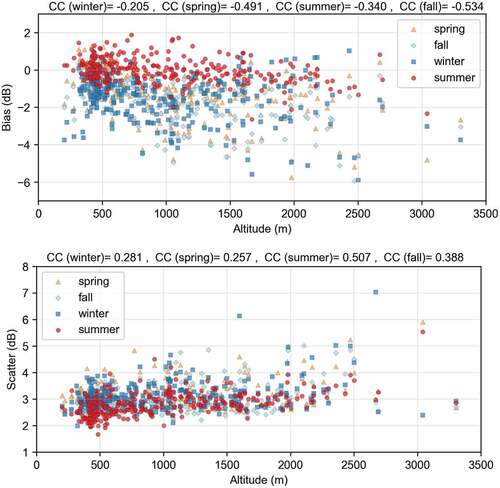
Table 1. Parameters of the linear regression between normalized altitude and RZC bias for different seasons (2016–2021). SE stands for the standard error of the regression parameters.

	CC	Slope ± SE	Intercept ± SE
All	−0.50	−0.71 ± 0.07	−0.82 ± 0.04
Summer	−0.34	−0.38 ± 0.06	−0.03 ± 0.04
Autumn	−0.53	−1.08 ± 0.10	−1.45 ± 0.06
Winter	−0.20	−0.41 ± 0.12	−1.57 ± 0.07
Spring	−0.49	−1.02 ± 0.11	−1.03 ± 0.07

Table 2. Parameters of the linear regression between normalized altitude and RZC scatter for different seasons (2016–2021). SE stands for the standard error of the regression parameters.

	CC	Slope ± SE	Intercept ± SE
All	0.45	0.38 ± 0.05	3.08 ± 0.03
Summer	0.51	0.39 ± 0.04	2.81 ± 0.02
Autumn	0.39	0.34 ± 0.05	2.97 ± 0.03
Winter	0.28	0.26 ± 0.05	3.13 ± 0.03
Spring	0.26	0.21 ± 0.05	3.14 ± 0.03

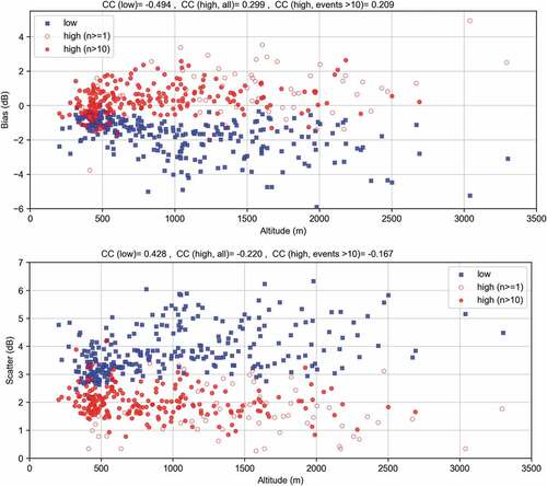
3.3. The role of precipitation intensity

In this section, we study the possible relation of precipitation intensity with the errors and the altitude of gauge measurements. Figure 6 shows the bias and the scatter for low and high intensities as functions of gauge altitudes. Bias tends to have a negative correlation with the gauge altitudes in the low-intensity threshold (explained variance of 24.4%). This means that in lower intensities, RZC tends to be characterized by larger underestimation at higher altitudes. Conversely, in the high-intensity threshold, radar tends to overestimate precipitation and it has very small correlation with altitude (explained variance of 9% for all gauges and 4% for gauges with $\mathit{n}>10$). Regarding the scatter, the error has a positive trend with the gauge altitudes in the low-intensity threshold and again a very weak correlation as the intensity increases. These results are in conjunction with section 3.2 (seasonality effect), as most high-intensity events are in heavy convective form during summer.

Figure 6. Total RZC bias (top) and scatter (bottom) as a function of the gauge altitudes for low and high intensities. Note that the red circle indicates the bias for the station which has more than 10 high intensity events.

The same approach is used for the CPC-CV product (Figure A4 in Appendix A): bias and scatter are clearly correlated with altitude in the low intensities. However, there is almost no correlation between residual errors and the gauge altitudes in higher intensities for CPC-CV.

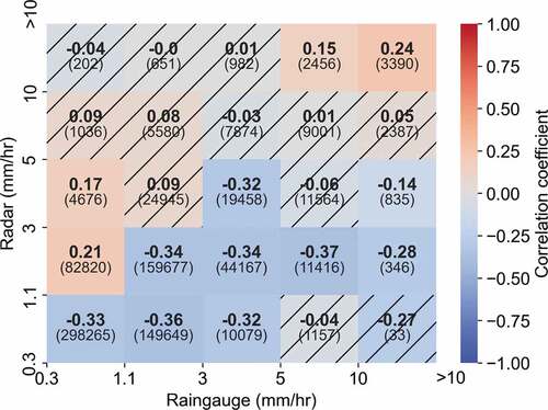
For the multi-threshold approach, Figure 7 shows the correlation between altitude and bias regarding different intensities estimated by gauges and radar products. Note that each value indicates the correlation value for the precipitation intensities between the current and the higher intensity category and its relation to the gauge altitudes. For instance, the value in the fourth row from the bottom and second column from the left (0.08) indicates the correlation for the bias of precipitation intensities between 1.1 and 3 $\mathit{mm}.h^{-1}$ measured by rain gauges and between 5 and 10 $\mathit{mm}.h^{-1}$ estimated by RZC. Note that for some categories, the p-values are significant and are hatched black in Figure 7. The results are in conjunction with one-threshold approach, i.e. noticeable negative correlation with altitude during the events which RZC underestimated precipitation. When both gauges and RZC products estimates are in the same category (diagonal which starts from bottom-left), there is a clear change in correlation from negative to positive with increasing intensity. For the future intensity-based studies, this approach can be used with larger data together with a multi-threshold contingency table to have a better picture of the interaction between gauge-radar intensities.

Figure 7. Correlation between altitude and bias for different intensity categories. Hatching indicates significant p-values. Numbers in parentheses indicate the total number of events in all stations in each category.

3.4. Comparison with snow measurements at the glaciers

Among 279 employed stations, there are 20 stations located at the altitude over 2000 m, and only five of them are located over 2500 m. To have a larger sample size in higher altitudes, we decided to use the snow depth measurements from eight glaciers over Switzerland. We refer to Gugerli et al. (2020) and Guidicelli et al. (2021) for more details information about these manual measurements. In summary, we have used the glaciological surveys obtained by GLAMOS at the end of the snow accumulation season (late spring) on all glaciers. The end-of-season snow accumulation observations by GLAMOS are conducted in spring around the peak of snow accumulation. Snow depth is obtained by snow probing throughout the glacier surface. One to several snow pits are dug on each glacier to derive a mean snow density (Bauder et al. 2018). Point observations of snow depth are multiplied by the average density measured in the snow pits (Huss, Dhulst, and Bauder 2015). Within the snow pits, a tube is used to derive snow density at different depths [see Gugerli et al. (2019) for more details]. We add these manual measurements to the gauge measurements of period 3 (2016–2021). Note that the snow season for these glaciers is considered to be seven months (October to April). Similarly, we use the gauge data of the stations above 2000 m from October to April, and for lower altitudes, we use the regular winter months (December to February). The bias values for the two products and glaciers are shown in Figures 8 and 9. To use the glacier data for the regression, we use the average height of each glacier (blue points in Figures 8 and 9), while some glaciers are extended at different altitudes (horizontal blue lines in the figures). The bias for the manual measurement of the glaciers has a fair agreement with the gauge measurements at high altitudes. As mentioned in section 3.2, bias correlation with altitude in winter is the weakest among other seasons. Adding the glacier data to increase the data points at higher altitudes could strengthen this correlation noticeably (Table 3). We emphasize that the type of these measurements is different from the usual gauge measures, which may affect the evaluation.

Figure 8. Total RZC bias as a function of the site altitudes without and with adding the data from glaciers. The blue points indicate the bias at the average altitudes of the glaciers and horizontal lines are the extent of each glacier’s altitude. The black vertical dash-line indicates the altitude where we separate winter into seven months (higher than 2000 m) and three months (below 2000 m).

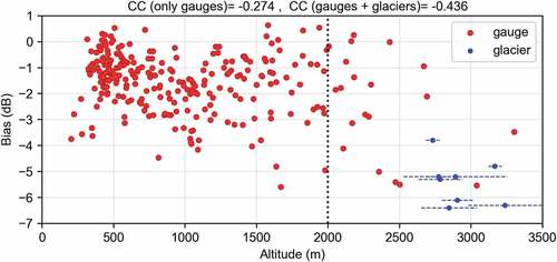
Figure 9. Same as Figure 8, but for CPC-CV products.

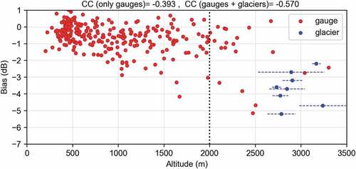
Table 3. Parameters of the linear regression between normalized altitude and bias without and with considering the snow measurement at the glaciers (2016–2021). SE stands for the standard error of the regression parameters.

	CC	Slope ± SE	Intercept ± SE
RZC with only gauges	−0.27	−0.55 ± 0.12	−1.59 ± 0.07
RZC with gauges and glaciers	−0.44	−0.87 ± 0.11	−1.65 ± 0.07
CPC-CV with only gauges	−0.39	−0.60 ± 0.09	−0.63 ± 0.05
CPC-CV with gauges and glaciers	−0.57	−1.02 ± 0.09	−0.71 ± 0.06

4. Discussion

The altitude of the gauge – as an indication of the depth of the growth layer – was found to be an important factor in gauge-radar errors (Gabella, Joss, and Perona 2000). However, this factor has not been separately considered and analysed using long-term data. Here, we considered 16 years of hourly precipitation data to study the relationship between the gauge altitude and gauge-radar errors over Switzerland. Based on the data for the entire 16 years, both radar products showed that the bias underestimation of precipitation and the dispersion of the error (scatter) increase with altitude. Several corrections have already been applied to the radar estimates and led to an overall improvement of the final products, including visibility correction, profile correction, and bias correction to generate the radar products in both old (Germann et al. 2006) and new radar networks (Germann et al. 2022). However, the results showed that the dependency of the gauge-radar errors with altitude is still present in both networks. For the CPC-CV product, bias and scatter errors were significantly reduced in most stations, and the regression model shows a milder bias gradient with altitude. This indicates that the leave-one-out cross-validation algorithm is a strong tool to dampen QPE errors, yet the altitudinal dependency of the scatter (dispersion around the mean) is still present.

Adding two more radars improved the final radar products in most stations by boosting the visibility of the radar network. This improvement is more significant for the stations closer to these two radars (Pointe de la Plaine Morte and Weissfluhgipfel). In a few stations, however, the bias has larger values in the new network. Besides the systematic errors in gauge measurements, which can lead to an increase in bias with higher precipitation amounts, this is partly due to the radar merging algorithm. For example, station GRH was mostly covered by the radar Monte Lema in the first period. Installing the two new radars, which have less visibility over this station, and merging their estimates to the final radar product could cause this increase in bias error. In addition, the regression parameters did not show a significant improvement regarding the dependency of bias and scatter on altitude for both radar products. Comparing RZC and CPC-CV products in the old and new radar networks confirms that the cross-validation algorithm is a powerful tool to reduce radar errors even with fewer single-polarization radars. This is particularly important for the regions where the hardware advancement has its physical or financial limitations, and therefore, using appropriate merging algorithms can significantly improve the radar precipitation estimates.

Based on the results, the altitudinal effect on the residual errors changes in different seasons. In winter, bias shows a larger underestimation in low altitudes compared to other seasons. This can be explained by the fact that overshooting is an important source of the error for QPE products in stratiform precipitation (Germann et al. 2022), particularly in winter when most of the events are less vertically developed and due to low-level clouds (Panziera et al. 2018). Another source of uncertainty in winter is more frequent snow, where the echoes are weak (Germann et al. 2022). This underestimation in low altitudes caused a poor correlation between bias and altitude in winter. On the contrary, radar products show overestimation in many stations in summer. The correction algorithm for the vertical profile of reflectivity, which is based on stratiform precipitation, can lead to the overestimation of QPE products in summer times (Germann et al. 2006). Both spring and autumn errors change between winter and summer error values due to the presence of convection in these seasons in parts of the country, such as southern parts of the Alps (Rudolph and Friedrich 2013). These results are comparable with Molnar and Burlando (2008), in which the summer season shows the shortest autocorrelation range due to convective activities, winter events are strongly autocorrelated due to larger-scale frontal events, and spring and fall events lay in between. Compared to RZC, the errors of CPC-CV products decreased in many stations, especially in lower altitudes in winter.

Our analysis showed a substantial effect of precipitation intensity on the radar errors and their relation with altitude. While bias in lower intensities shows a strong negative correlation with altitude, a poor positive correlation was observed for higher intensities. This is because most of the high-intensity events in an hourly timescale are in a convective form, also mentioned for the seasonality effect. These results are similar to Barton et al. (2020), where the sub-hourly precipitation data had a negative bias underestimation for low intensities and overestimation for high-intensity values, particularly during the warm season. Here, the cross-validated algorithm could also reduce bias and scatter errors in low and high-intensity events for many stations. This reduction of the errors considerably diminished the altitudinal dependency in high intensities.

Manual snow measurements from eight glaciers showed considerably higher values than radar products over these glaciers as well as the gauges at similar altitudes. Like other measuring techniques, these manual measurements have limitations, such as low temporal resolution and the representativeness error of the point measurements for larger areas of the glacier (Grünewald and Lehning 2015). However, bias error represents the accumulated error over the time period (six years in our study), and the glacier-wide deviation of the overall mean field bias is small (Gugerli et al. 2020). Considering the effect of wind under-catch on the gauge measurements at higher altitudes (Pollock et al. 2018), the actual underestimation of radar could be even larger at these altitudes. The bias showed a clear dependency on altitude for both radar products when using both manual and gauge measurements in winter. Despite the gauge systematic errors due to wind under-catch, CPC-CV could dampen the bias error over the glaciers in winter. We cautiously conclude that using the cross-validation algorithm can partly improve radar errors in estimating accumulated snow. However, more studies are required to have a robust conclusion regarding snow estimates at high altitudes. As expected, the regression showed steeper slopes by adding the glacier data for both RZC and CPC-CV.

In general, the cross-validation algorithm is shown to be a powerful tool for improving radar estimates over Switzerland in different seasons. The radar residual errors showed a clear correlation with gauge altitudes over Switzerland. Almost 30% of both error metrics (bias and scatter) in the two radar products can be statistically explained using the gauge altitudes as a single explanatory variable. Although many factors affect the estimation errors in mountainous areas, a simple regression model with gauge altitudes as a predictor performs reasonably well in explaining gauge-radar variability. However, some limitations are worth noting. Despite all the advantages of using long-term data for analysing precipitation estimates, some anomalous behaviours (such as significant overestimation in a few events) might be missed and neutralized by overall underestimation. Although we studied the effect of altitude based on different seasons and intensities, this effect has not been separately studied based on different precipitation regimes and their duration. These factors – which are related to the atmospheric processes – impact the precipitation amount in regional scales (Allamano et al. 2009; Formetta et al. 2022). To cover the physical processes, future studies should include these parameters in regional scales. Considering the aforementioned limitations, the results of this study can be used to include a correction factor for QPE products based on altitude and precipitation intensity in different seasons. We also suggest studying the relationship between altitude and radar errors over different mountainous regions.

5. Conclusions

We studied the relationship between the residual errors of Quantitative Precipitation Estimates (QPE) and the altitude of the gauges over Switzerland using 16 years of hourly precipitation data. We calculated radar residual errors over Switzerland as the two log-transformed metrics (bias and scatter) for two QPE products using the gauges as a reference. The radar-only (RZC) and cross-validated-merged-with-gauge (CPC-CV) products are generated by MeteoSwiss and used in this study. The results can be summarized as follows:

• Overall, the results showed a clear dependency of the residual errors with the gauge altitudes during these 16 years for both radar products. The bias showed −0.56 and −0.48 Pearson correlation with the gauge altitudes for RZC and CPC-CV products, respectively. The correlation of the scatter with altitude for RZC product was+0.57 and for CPC-CV was+0.61. These results indicate an increase in the error dispersion as well as a larger underestimation at higher altitudes in both products. For CPC-CV, both components of the residual errors show lower values than RZC in most stations. However, increasing the errors with altitude is still noticeable.

• Since the network improved during these 16 years, we analyzed the effect of the old (3 radars) and the new (5 radars) networks. Although using the new radar network led to an error reduction, the relationship between altitude and errors is still present. Even a simple linear regression model performs reasonably well in explaining the altitudinal dependency of both error components in the new radar network.

• We considered each season individually to check possible seasonal effects on the error-altitude relationship. Based on these results, during winter season, both metrics already had high values in low altitudes, possibly due to the more frequent snowfall and the low-altitude clouds in winter. This led to the weakest bias correlation (−0.2) in winter. Despite other seasons, during summer, almost half of the stations (mostly located below 1500 m) overestimated precipitation with the bias correlation of −0.34 with altitude. In terms of scatter, summer precipitation showed lower values, especially in low altitudes, and the strongest correlation than other seasons (+0.51). Using the CPC-CV algorithm could reduce the errors in low altitudes, especially in winter. Having a higher correlation for CPC-CV, especially in winter, indicates that considering an altitudinal factor in the algorithm can reduce the errors at high altitudes.

• Furthermore, we studied the effect of precipitation intensity on the error-altitude relationship using single and multi-threshold approaches. The results for the single threshold approach showed a systematic underestimation of the two QPE products for low intensities (below 1.1 $\mathit{mm}.h^{-1}$) with a clear negative correlation of bias with gauge altitudes (−0.49). Despite most of the findings, radar products mostly overestimate precipitation for high intensities (above 7 $\mathit{mm}.h^{-1}$) with a weak positive correlation of bias with the gauge altitudes (0.21). For scatter, there is a clear positive trend in the low intensities. In contrast, for high intensities, we found that the scatter does not increase with altitude, even decreases in some stations. Also, we tried to explain the relationship between intensity, the errors, and the gauge altitudes by dividing precipitation into 25 gauge-radar intensity categories. Generally, the results showed a similar trend with the two-threshold approach. Furthermore, a clear negative correlation with altitude was observed when the QPE products underestimated precipitation.

• Lastly, we used snow measurements from 8 glaciers in Switzerland in combination with the gauge data for seven months to increase the sample size of the observations at higher altitudes. Adding these measurements strengthened the negative correlation for the bias error in both QPE products during the winter season. However, it should be mentioned that these manual measurements are different from the gauge data and more detailed studies are needed for a robust conclusion to consider these measurements for this purpose.

Disclosure statement

No potential conflict of interest was reported by the authors.

Data availability statement

RZC and CPC-CV products as well as rain-gauge measurements are freely available at MeteoSwiss. Glaciological surveys of GLAMOS are freely available at https://www.glamos.ch/en/.

Additional information

Funding

This work is funded by the Austrian Science Fund (FWF) under research grant W1256 (doctoral program Climate Change – Uncertainties, Thresholds and Coping Strategies)

Appendix A

Table A1. Parameters of the linear regression between normalized altitude and bias from 2005 to 2021. SE stands for the standard error of the regression parameters.

	CC	Slope ± SE	Intercept ± SE
RZC (all)	−0.56	−0.86 ± 0.08	−1.01 ± 0.05
CPC-CV (all)	−0.48	−0.56 ± 0.06	−0.54 ± 0.04
RZC (2016–2021)	−0.50	−0.71 ± 0.07	−0.82 ± 0.04
CPC-CV (2016–2021)	−0.51	−0.58 ± 0.06	−0.46 ± 0.04

Table A2. Parameters of the linear regression between normalized altitude and scatter from 2005 to 2021. SE stands for the standard error of the regression parameters.

	CC	Slope ± SE	Intercept ± SE
RZC (all)	0.57	0.58 ± 0.05	3.27 ± 0.03
CPC-CV (all)	0.61	0.63 ± 0.05	2.15 ± 0.03
RZC (2016–2021)	0.45	0.38 ± 0.05	3.08 ± 0.03
CPC-CV (2016–2021)	0.62	0.58 ± 0.04	2.00 ± 0.03

Figure A1. Bias (top) and scatter (bottom) for CPC-CV products from 2016 to 2021. Note that the yellow triangular symbols show the location of the radars and the map extends from 5.53^° E and 45.46^° N (bottom left) to 10.38^° E to 47.48^° N (top right) in World Geodetic System (Wgs84).

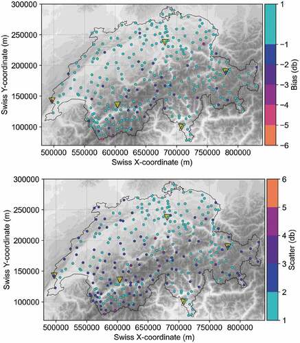
Table A3. Parameters of the linear regression between normalized altitude and bias for the old and new radar network using the same 72 stations. SE stands for the standard error of the regression parameters.

	CC	Slope ± SE	Intercept ± SE
RZC (2005–2010)	−0.48	−1.07 ± 0.24	−0.88 ± 0.17
CPC-CV (2005–2011)	−0.35	−0.58 ± 0.19	−0.88 ± 0.13
RZC (2016–2021)	−0.62	−0.94 ± 0.14	−0.87 ± 0.1
CPC-CV (2016–2021)	−0.60	−0.85 ± 0.14	−0.54 ± 0.1

Table A4. Parameters of the linear regression between normalized altitude and scatter for the old and new radar network using 72 stations. SE stands for the standard error of the regression parameters.

	CC	Slope ± SE	Intercept ± SE
RZC (2005–2010)	0.63	0.97 ± 0.14	3.58 ± 0.1
CPC-CV (2005–2010)	0.67	0.78 ± 0.1	2.66 ± 0.07
RZC (2016–2021)	0.57	0.48 ± 0.08	3.15 ± 0.06
CPC-CV (2016–2021)	0.67	0.7 ± 0.09	2.06 ± 0.07

Figure A2. Bias (top) and scatter (bottom) for the same 72 stations in the old (left) and new (right) radar networks. Note that the yellow triangular symbols show the location of the radars and the map extends from 5.53^° E and 45.46^° N (bottom left) to 10.38^° E to 47.48^° N (top right) in World Geodetic System (WGS84).

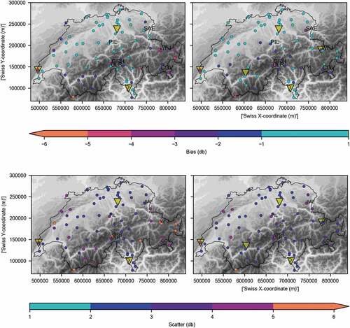
Figure A3. Total CPC-CV bias (top) and scatter (bottom) from 2016 to 2021 as a function of the gauge altitudes for different seasons.

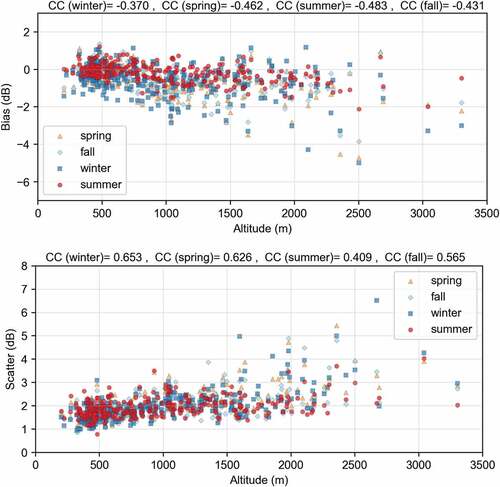
Figure A4. Total CPC-CV bias (top) and scatter (bottom) as a function of the gauge altitudes for low and high intensities. Note that the red circles indicates the bias for the station which has more than 10 high intensity events.

References

- Allamano, P., P. Claps, F. Laio, and C. Thea. 2009. “A Data-Based Assessment of the Dependence of Short-Duration Precipitation on Elevation.” Physics and Chemistry of the Earth, Parts A/B/C 34 (10–12): 635–641. doi:10.1016/j.pce.2009.01.001.
- Barton, Y., I. V. Sideris, T. H. Raupach, M. Gabella, U. Germann, and O. Martius. 2020. “A Multi-Year Assessment of Sub-Hourly Gridded Precipitation for Switzerland Based on a Blended Radar—Rain-gauge Dataset.” International Journal of Climatology 40 (12): 5208–5222. doi:10.1002/joc.6514.
- Bauder, A., M. Funk, M. Huss, G. Kappenberger, A. Linsbauer, and U. Steinegger 2018. Glamos. the Swiss Glaciers 2015/16 and 2016/17. Glaciological Report No. 137/138. The Swiss Glaciers. Glaciological Report 137.
- Benoit, K. 2011. “Linear Regression Models with Logarithmic Transformations.” London School of Economics London 22(1): 23–36
- Berne, A., and W. F. Krajewski. 2013. “Radar for Hydrology: Unfulfilled Promise or Unrecognized Potential?” Advances in Water Resources 51: 357–366. doi:10.1016/j.advwatres.2012.05.005.
- Cecinati, F., M. A. Rico-Ramirez, G. B. Heuvelink, and D. Han. 2017. “Representing Radar Rainfall Uncertainty with Ensembles Based on a Time-Variant Geostatistical Error Modelling Approach.” Journal of Hydrology 548: 391–405. doi:10.1016/j.jhydrol.2017.02.053.
- Ciach, G. J., W. F. Krajewski, and G. Villarini. 2007. “Product-Error-Driven Uncertainty Model for Probabilistic Quantitative Precipitation Estimation with Nexrad Data.” Journal of Hydrometeorology 8 (6): 1325–1347. doi:10.1175/2007JHM814.1.
- Faure, D., G. Delrieu, and N. Gaussiat. 2019. “Impact of the Altitudinal Gradients of Precipitation on the Radar Qpe Bias in the French Alps.” Atmosphere 10 (6): 306. doi:10.3390/atmos10060306.
- Formetta, G., F. Marra, E. Dallan, M. Zaramella, and M. Borga. 2022. “Differential Orographic Impact on Sub-Hourly, Hourly, and Daily Extreme Precipitation.” Advances in Water Resources 159: 104085. doi:10.1016/j.advwatres.2021.104085.
- Frei, C., and C. Schär. 1998. “A Precipitation Climatology of the Alps from High-Resolution Rain-Gauge Observations.” International Journal of Climatology: A Journal of the Royal Meteorological Society 18 (8): 873–900. doi:10.1002/(SICI)1097-0088(19980630)18:8<873:AID-JOC255>3.0.CO;2-9.
- Gabella, M., J. Joss, and G. Perona. 2000. “Optimizing Quantitative Precipitation Estimates Using a Noncoherent and a Coherent Radar Operating on the Same Area.” Journal of Geophysical Research Atmospheres 105 (D2): 2237–2245. doi:10.1029/1999JD900420.
- Gabella, M., J. Joss, G. Perona, and S. Michaelides. 2005. “Range Adjustment for Ground-Based Radar, Derived with the Spaceborne Trmm Precipitation Radar.” IEEE Transactions on Geoscience and Remote Sensing 44 (1): 126–133. doi:10.1109/TGRS.2005.858436.
- Gabella, M., and R. Notarpietro. 2004. “Improving Operational Measurement of Precipitation Using Radar in Mountainous Terrain-Part I: Methods.” IEEE Geoscience and Remote Sensing Letters 1 (2): 78–83. doi:10.1109/LGRS.2003.822311.
- Gabella, M., P. Speirs, U. Hamann, U. Germann, and A. Berne. 2017. “Measurement of Precipitation in the Alps Using Dual-Polarization C-Band Ground-Based Radars, the Gpm Spaceborne Ku-Band Radar, and Rain Gauges.” Remote Sensing 9 (11): 1147. doi:10.3390/rs9111147.
- Germann, U., M. Berenguer, D. Sempere-Torres, and M. Zappa. 2009. “Real—Ensemble Radar Precipitation Estimation for Hydrology in a Mountainous Region.” Quarterly Journal of the Royal Meteorological Society: A Journal of the Atmospheric Sciences, Applied Meteorology and Physical Oceanography 135 (639): 445–456. doi:10.1002/qj.375.
- Germann, U., M. Boscacci, L. Clementi, M. Gabella, A. Hering, M. Sartori, I. V. Sideris, and B. Calpini. 2022. “Weather Radar in Complex Orography.” Remote Sensing 14 (3): 503. doi:10.3390/rs14030503.
- Germann, U., G. Galli, M. Boscacci, and M. Bolliger. 2006. “Radar Precipitation Measurement in a Mountainous Region.” Quarterly Journal of the Royal Meteorological Society: A Journal of the Atmospheric Sciences, Applied Meteorology and Physical Oceanography 132 (618): 1669–1692.
- Germann, U., G. Galli, M. Boscacci, M. Bolliger, and M. Gabella. 2004. “Quantitative Precipitation Estimation in the Alps: Where Do We Stand?” ERAD Publication Series 2: 2–6.
- Grünewald, T., and M. Lehning. 2011. “Altitudinal Dependency of Snow Amounts in Two Small Alpine Catchments: Can Catchment-Wide Snow Amounts Be Estimated via Single Snow or Precipitation Stations?” Annals of Glaciology 52 (58): 153–158.
- Grünewald, T., and M. Lehning. 2015. “Are Flat-Field Snow Depth Measurements Representative? A Comparison of Selected Index Sites with Areal Snow Depth Measurements at the Small Catchment Scale.” Hydrological Processes 29 (7): 1717–1728.
- Grüter, E., M. Abbt, C. Häberli, E. Haller, U. Küng, M. Musa, T. Konzelmann, and R. Dössegger 2003. Quality Control Tools for Meteorological Data in the Meteoswiss Data Warehouse System. Technical report, Internal report, MeteoSwiss: Zürich.
- Gugerli, R., M. Gabella, M. Huss, and N. Salzmann. 2020. “Can Weather Radars Be Used to Estimate Snow Accumulation on Alpine Glaciers? An Evaluation Based on Glaciological Surveys.” Journal of Hydrometeorology 21 (12): 2943–2962.
- Gugerli, R., N. Salzmann, M. Huss, and D. Desilets. 2019. “Continuous and Autonomous Snow Water Equivalent Measurements by a Cosmic Ray Sensor on an Alpine Glacier.” The Cryosphere 13 (12): 3413–3434.
- Guidicelli, M., R. Gugerli, M. Gabella, C. Marty, and N. Salzmann. 2021. “Continuous Spatio-Temporal High-Resolution Estimates of Swe Across the Swiss Alps–A Statistical Two-Step Approach for High-Mountain Topography.” Frontiers in Earth Science 9: 664648.
- Haiden, T., A. Kann, C. Wittmann, G. Pistotnik, B. Bica, and C. Gruber. 2011. “The Integrated Nowcasting Through Comprehensive Analysis (Inca) System and Its Validation Over the Eastern Alpine Region.” Weather and Forecasting 26 (2): 166–183.
- Huss, M., L. Dhulst, and A. Bauder. 2015. “New Long-Term Mass-Balance Series for the Swiss Alps.” Journal of Glaciology 61 (227): 551–562.
- Kann, A., I. Meirold-Mautner, F. Schmid, G. Kirchengast, J. Fuchsberger, V. Meyer, L. Tüchler, and B. Bica. 2015. “Evaluation of High-Resolution Precipitation Analyses Using a Dense Station Network.” Hydrology and Earth System Sciences 19 (3): 1547–1559.
- Krajewski, W. F. 1987. “Cokriging Radar-Rainfall and Rain Gage Data.” Journal of Geophysical Research Atmospheres 92 (D8): 9571–9580.
- Le Bastard, T., O. Caumont, N. Gaussiat, and F. Karbou. 2019. “Combined Use of Volume Radar Observations and High-Resolution Numerical Weather Predictions to Estimate Precipitation at the Ground: Methodology and Proof of Concept.” Atmospheric Measurement Techniques 12 (10): 5669–5684.
- Masson, D., and C. Frei. 2014. “Spatial Analysis of Precipitation in a High-Mountain Region: Exploring Methods with Multi-Scale Topographic Predictors and Circulation Types.” Hydrology and Earth System Sciences 18 (11): 4543–4563.
- Molnar, P., and P. Burlando. 2008. “Variability in the Scale Properties of High-Resolution Precipitation Data in the Alpine Climate of Switzerland.” Water Resources Research 44 (10): W10404–1.
- Panziera, L., M. Gabella, U. Germann, and O. Martius. 2018. “A 12-Year Radar-Based Climatology of Daily and Sub-Daily Extreme Precipitation Over the Swiss Alps.” International Journal of Climatology 38 (10): 3749–3769.
- Pollock, M. D., G. O’Donnell, P. Quinn, M. Dutton, A. Black, M. Wilkinson, M. Colli, M. Stagnaro, L. Lanza, E. Lewis, Kilsby, C., O’Connell, P., et al. 2018. “Quantifying and Mitigating Wind-Induced Undercatch in Rainfall Measurements.” Water Resources Research 54 (6): 3863–3875.
- Pulkkinen, S., D. Nerini, A. A. Pérez Hortal, C. Velasco-Forero, A. Seed, U. Germann, and L. Foresti. 2019. “Pysteps: An Open-Source Python Library for Probabilistic Precipitation Nowcasting (V1. 0).” Geoscientific Model Development 12 (10): 4185–4219.
- Rudolph, J. V., and K. Friedrich. 2013. “Seasonality of Vertical Structure in Radar-Observed Precipitation Over Southern Switzerland.” Journal of Hydrometeorology 14 (1): 318–330.
- Schwarb, M. 2000. The Alpine precipitation climate: evaluation of a high-resolution analysis scheme using comprehensive rain-gauge data. Ph. D. thesis, ETH Zurich.
- Seo, D. -J., and J. Breidenbach. 2002. “Real-Time Correction of Spatially Nonuniform Bias in Radar Rainfall Data Using Rain Gauge Measurements.” Journal of Hydrometeorology 3 (2): 93–111.
- Sevruk, B. 1997. “Regional Dependency of Precipitation-Altitude Relationship in the Swiss Alps.” Climatic Change 36: 355–369.
- Sideris, I., M. Gabella, R. Erdin, and U. Germann. 2014. “Real-Time Radar–rain-Gauge Merging Using Spatio-Temporal Co-Kriging with External Drift in the Alpine Terrain of Switzerland.” Quarterly Journal of the Royal Meteorological Society. 140 (680): 1097–1111.
- Sokol, Z., and V. Bližňák. 2009. “Areal Distribution and Precipitation–Altitude Relationship of Heavy Short-Term Precipitation in the Czech Republic in the Warm Part of the Year.” Atmospheric Research 94 (4): 652–662.
- Wolfensberger, D., M. Gabella, M. Boscacci, U. Germann, and A. Berne. 2021. “Rainforest: A Random Forest Algorithm for Quantitative Precipitation Estimation Over Switzerland.” Atmospheric Measurement Techniques 14 (4): 3169–3193.