The built-up environment modulates the association of artificial night-time lights with the urban extent

ABSTRACT

Artificial night-time light (NTL) emissions, collected by satellites, are a reliable and widely used remote proxy for urban extent. Recently, it was demonstrated that NTLs are stronger associated with the total volume of the buildings than with their total footprint area, a traditional urban extent measure. However, this finding may not be a general rule: We presume that both associations are sensitive to characteristics of the built-up environment, while the latter is known to be quite heterogeneous within and between cities. Moreover, we hypothesize that at least in specific built-up environments, NTL may even stronger correlate with another urban extent measure – the total lateral surface area of the buildings, due to its more accurate proportionality to the area of light-emitting windows. The present study uses NTLs and buildings datasets of 38 European capital cities and compares the associations of NTLs with the three aforementioned urban extent measures (the total footprint area, the total volume, and the total lateral surface area of the buildings) across different built-up environments. The results indicate that in urban areas characterized by a high density of tall buildings the strongest observed association is between NTLs and the building’s footprint area. In comparison, the total volume of buildings is better related to NTLs in urban areas that host compact settings of relatively small buildings. But there is a third type of physical urban configuration, characterized by large buildings sparsely distributed in space. In this type of urban area, the strongest observed association is between NTLs and lateral surface area. We conclude that monitoring urban growth using NTLs will benefit from a preliminary assessment of the local built-up characteristics.

KEYWORDS:

• Artificial night-time light (NTL)
• urban extent
• total footprint area
• total volume
• total lateral surface area
• built-up environment characteristics

1. Introduction

Emissions of artificial night-time light (NTL) are often used as a proxy for human presence on the Earth generally (Doll, Muller, and Elvidge 2000; Ebener et al. 2005; Elvidge et al. 1997; Hopkins et al. 2018; Ma et al. 2012; Mellander et al. 2015) and for urban extent specifically (Dou et al. 2017; He et al. 2006; Henderson et al. 2003; Imhoff et al. 1997; Liu et al. 2012; Rybnikova et al. 2021; K. Shi et al. 2014). A traditional approach explains the variation of NTLs across urban sites by the variation of the total footprint area of buildings located on the site (L. Shi et al. 2020). In their recent article, Shi with co-authors explore the urban areas located in the UK, in the US, and across countries of the European Union (L. Shi et al. 2020). The authors argue that the total NTLs emitted from urban sites better correlate with the total volume of the buildings, compared to just their total footprint area. However, the built-up environments within even a small study area might be essentially different in terms of the buildings’ size, disposition, density, etc. This, in turn, might determine which of the mentioned urban extent measures is more appropriate. For example, in a dense configuration of similarly high buildings, most of the emitted light will be absorbed by neighbouring buildings. In this case, the advantage of the ‘NTLs-buildings’ volume” correlation over the alternative ‘NTLs-footprint area’, may depend on the predominant height of the buildings. However, in sparse urban configurations, characterized by relatively dispersed buildings, the light emitted through the building’s windows has a better chance to be observable from above. We hypothesize that, in these cases, NTLs will better correlate with the lateral surface area of the buildings, rather than with their footprint area and volume. The first aim of the present study is to test the posed hypothesis. If it is confirmed, we aim to define general guidelines for choosing the urban extent measure (footprint area, volume, or lateral surface area) that would fit the local built-up environment the best.

In the present study, we compare NTLs emitted from the urban cores of the European capital cities with the three alternative urban extent measures. The pixels of the NTL satellite image are treated as the observation units. For each pixel, we calculate: (i) alternative urban extent measures – by summing up footprint area, volumes, or lateral surface areas of all buildings within the pixel, and (ii) characteristics of the built-up environment – by averaging buildings’ shape, disposition, and density. We first perform a pooled analysis by assessing the ‘NTL – footprint area’, ‘NTL – volume’, and ‘NTL – lateral surface area’ associations for the whole dataset of pixels. Second, we divide the pool of pixels into classes based on the considered characteristics of the built-up environment and re-assess the examined associations separately for each group of pixels. We point out the groups in which NTLs stronger correlate with either the total footprint area, total volume, or total lateral surface area. Finally, we validate the obtained results at the level of entire city areas – to check whether it is plausible to choose a universal superior urban extent measure.

The obtained results indicate that certain built-up characteristics, such as average buildings’ footprint size and proximity to other buildings, indeed affect the associations of NTLs with urban extent measures, which makes each of them appropriate for different sites and cities. We believe that this finding is practically important for monitoring urban dynamics via NTLs since it sheds light on the inaccuracies of the NTL-based estimates of urban extent obtained by non-appropriate measures.

2. Materials and methods

We proceed from the two data sources. The first one refers to the Urban Atlas, reporting the footprints of buildings for European cities as polygon shapefiles, and the heights of buildings within the cities’ urban core areas as raster layers of 10-metre resolution (EEA 2023a). These data are generated from stereo images and digital surface/terrain models (EEA 2023b) and are available only for 2012. The second data source is a VNL V2 product for NTL radiance, provided by the Visible Infrared Imaging Radiometer Suite Day/Night Band (VIIRS/DNB) (EOG 2023). The NTL radiance from VIIRS/DNB is available from 2012 onward, but to assure correspondence between both data sources, only the data for 2012 was used. NTL data is a raster layer reporting by each its pixel total light emissions in 10⁻⁹ W cm⁻² sr⁻¹ units from the areas of 15 arc seconds, which is ~0.5 km² at the Equator (EOG 2023). To ensure comparability of the total lights emitted from the areas of different latitudes, we applied a latitude-correction procedure, multiplying each NTL value by the cosine of the corresponding pixel centroid’s latitude.

In the analysis, we examined the urban cores of the 38 European capital cities. From each core, we extracted a central rectangular area of ~ 20×10 km, corresponding to ~ 40×20 pixels of the NTL raster layer (the data are available from the authors upon request). For each pixel, we calculated three alternative urban extent measures, adding up the relevant parameter of all the buildings located in the specific pixel: Footprint area, volume, or lateral area. Therefore, each pixel has its own total footprint area, total volume, and total lateral surface area. We then estimated the correlations between VIIRS/DNB-provided NTL radiance and each of the three measures, using Kendall’s tau-b coefficient as the most robust non-parametric correlation metric (Tay 2023).

Afterward, for each pixel, we calculated various characteristics of the built-up environment: the average density of the built-up area, the average proximity to the neighbouring building, and the average footprint area, perimeter, height, and compactness of the buildings hosted by the pixel. The concept of compactness refers to a unitless measure that compares the area of a shape with an area of an ‘ideal’ shape, considered the most compact (Marshall, Gong, and Green 2019; Montero and Bribiesca 2009). In the present analysis, we calculated two types of compactness for buildings: 2D compactness is defined as a ratio of the building footprint area to the area of a square of the same perimeter (the square was chosen as an ‘ideal’ rectangular). The second type is 3D compactness: The ratio of the building’s volume to the volume of a cube of the same lateral surface (in this case, the cube was chosen as an ‘ideal’ parallelepiped).

Based on each of the examined built-up characteristics, we divided the full set of observations into five groups and re-assessed the ‘NTL – footprint area’, ‘NTL – volume’, and ‘NTL – lateral surface area’ correlations for each of the groups. While classifying the dataset, common classification techniques were used: (i) geometrical interval classification, implying a minimization of the within-class variances for non-normally distributed data (ESRI 2023); (ii) quantile classification, implying an equal number of observations in each class; and (iii) equal interval classification, implying splitting the parameter range (but not the number of observations) into equal intervals. The three examined classification techniques cover essentially different grouping approaches, either by ‘natural’ patterns inherent in the data, by the equal number of observations, or by the equal difference between the highest and lowest parameter level. These grouping approaches are used to explore different subsets of observations with stronger associations between NTLs and either total footprint, volume, or lateral surface area. Table 1 includes the descriptive statistics of the analysis.

Table 1. Descriptive statistics of the pooled set of observations (N = 23,690 pixels).

Variable	Descriptive statistics:
	Mean	Median	Std. Error
Sum of NTLs (10^−9 W cm^−2 sr^−1)	21.41	17.56	0.10
Measures of urban extent
Sum of footprint areas of buildings (m^2)	18,761.26	13,612.54	113.37
Sum of volumes of buildings (m^3)	283,832.13	143,826.10	2371.98
Sum of lateral surface areas of buildings (m^2)	57,613.14	27,244.80	493.38
Characteristics of the built-up environment
Number of buildings per pixel	57.86	31.00	0.49
Average distance between the neighbouring buildings (dd)	8.70·10^−5	5.34·10^−5	8.25·10^−8
Average footprint area of buildings (m^2)	723.39	368.02	13.77
Average footprint perimeter of buildings (m)	102.25	82.02	0.54
Average height of buildings (m)	11.10	9.33	0.04
Average 2D compactness of buildings (ratio)	0.80	0.81	7.80·10^−4
Average 3D compactness of buildings (ratio)	0.79	0.81	7.15·10^−4

Afterward, for different subsets of observations (i.e. those with certain levels of built-up characteristics), we assessed potential inaccuracies of the urban extent estimates caused by using a non-appropriate measure. To this end, for each subset, we run bivariate linear log-log models to predict alternative urban extent measures (the total footprint area, the total volume, or the total lateral surface area) from NTL intensities. By comparing the three obtained regression coefficients, we derived the levels of under/overestimation of urban extent given the use of a non-appropriate urban extent measure.

Finally, to evaluate whether the obtained results remain applicable to extensive urban areas, we perform a similar analysis at the level of entire cities: For each city, we calculate the ‘NTL – footprint area’, ‘NTL – volume’, and ‘NTL-lateral surface area’ associations. We divide the cities into groups by the superior association and analyse in terms of which built-up characteristics the groups significantly differ.

The analysis was performed in ArcGIS v.10.5 (ESRI 2021), SPSS v.25 (IBM 2020), and Matlab v.R2020 (MathWorks 2021) software.

3. Results

3.1. Associations of NTLs with alternative urban extent measures

For the pooled dataset consisting of 23,690 observations, the association between NTLs and the total volume of the buildings emerged the strongest (with the non-parametric Kendall’s tau-b correlation coefficient of 0.366), while the associations with footprint area and lateral surface area were somewhat weaker (with Kendall’s tau-b of 0.325 and 0.320, respectively).

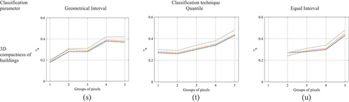
Table 2 describes the groups of pixels obtained from classifying the whole dataset by different built-up environment characteristics using different classification techniques. Figure 1, in the meantime, reports Kendall’s tau-b correlation coefficients for ‘NTL – footprint area’, ‘NTL – volume’, and ‘NTL – lateral surface area’ associations for each of the defined groups. As can be noticed from the figure, for the majority of cases, grey lines lie higher, indicating that the ‘NTL – volume’ association emerges the strongest.

Figure 1a. Kendall’s tau-b correlation coefficients (y-axes) between NTLs and the three urban extent measures: the total footprint area (blue lines), the total volume (grey lines), and the total lateral surface area (orange lines) of the buildings. The correlations are estimated for five groups of pixels (x-axes), arranged in ascending order by the values of the built-up environment characteristics.

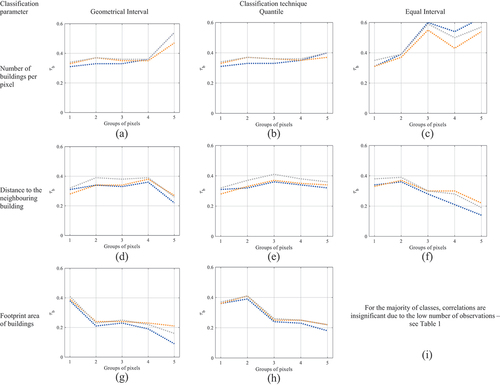
Table 2. Groups of observations derived from the whole dataset classification by different built-up environment characteristics using different classification techniques.

Class number	Built-up environment characteristics
	Number of buildings per pixel		Distance to the neighbour (dd)		Footprint area (m^2)		Footprint perimeter (m)		Height (m)		2D compactness (ratio)		3D compactness (ratio)
	N	Range	N	Range	N	Range	N	Range	N	Range	N	Range	N	Range
Geometrical Interval classification technique
#1	4,293	<7	5,071	<0.1·10^−4	11,972	<373	7,013	<62	8,646	<8	403	<0.48	177	<0.42
#2	5,348	[7–22)	6,380	[0.1·10^−4-0.5·10^−4)	553	[373–394)	2,110	[62–70)	1,202	[8–9)	1,688	[0.48–0.64)	2,356	[0.42–0.66)
#3	7,644	[22–70)	8,602	[0.5·10^−4-1.4·10^−4)	5,993	[394–762)	8,861	[70–122)	6,563	[9–13)	1,920	[0.64–0.69)	10,768	[0.66–0.82)
#4	5,276	[70–216)	2,836	[1.4·10^−4-3.6·10^−4)	5,009	[762–7,285)	5,505	[122–435)	7,258	[13–51)	10,312	[0.69–0.84)	9,427	[0.82–0.93)
#5	1,129	≥216	801	≥3.6·10^−4	163	≥7,285	201	≥435	21	≥51	9,367	≥0.84	962	≥0.93
Quantile classification technique
#1	4,755	<8	4,719	<0.1·10^−4	4,738	<170	4,737	<54	4,736	<7	4,736	<0.70	4,738	<0.72
#2	4,886	[8–22)	4,810	[0.1·10^−4-0.4·10^−4)	4,738	[170–289)	4,737	[54–72)	4,835	[7–8)	4,741	[0.70–0.78)	4,742	[0.72–0.78)
#3	4,687	[22–45)	4,722	[0.4·10^−4-0.7·10^−4)	4,738	[289–463)	4,738	[72–95)	4,807	[8–11)	4,736	[0.78–0.84)	4,727	[0.78–0.83)
#4	4,687	[45–92)	4,675	[0.7·10^−4-1.2·10^−4)	4,737	[463–817)	4,739	[95–132)	4,654	[11–16)	4,740	[0.84–0.90)	4,742	[0.83–0.88)
#5	4,675	≥92	4,764	≥1.2·10^−4	4,739	≥817	4,739	≥132	4,658	≥16	4,737	≥0.90	4,741	≥0.88
Equal Interval classification technique
#1	21,040	<135	21,305	<1.8·10^−4	23,661	<24,007	23,051	<280	23,686	<74	76	<0.24	76	<0.19
#2	1,948	[135–268)	1,584	[1.8·10^−4-3.6·10^−4)	23	[24,007–49,349)	544	[280–560)	3	[74–148)	587	[0.24–0.49)	587	[0.19–0.37)
#3	540	[268–400)	362	[3.6·10^−4-5.4·10^−4)	2	[49,349–60,508)	56	[560–840)	0	[148–222)	9,022	[0.49–0.73)	9,022	[0.37–0.62)
#4	131	[400–533)	122	[5.4·10^−4-7.2·10^−4)	2	[60,508–90,200)	19	[840–1120)	0	[222–296)	13,938	[0.73–0.98)	13,938	[0.62–0.86)
#5	31	≥533	317	≥7.2·10^−4	2	≥90,200	20	≥1120	1	≥370	67	≥0.98	67	≥0.86

In a few cases, the ‘NTL – lateral surface area’ association outcompeted the two others (see orange lines in Figure 1(d-i). These cases represent two types of sites. The first are sites hosting buildings with the largest footprints – with an average area exceeding 7,285 m² (Figure 1(g)) or with an average perimeter over 560 m (Figure 1(i). The second are the most sparsely built sites – with an average distance between the closest neighbours over 3.6·10⁻⁴ dd (Figure 1(d) (interestingly, picking up the cases with further larger between-building distance – with over 3.5·10⁻⁴ and 7.2·10⁻⁴ dd – results in even more convincing advantage of the ‘NTL – lateral surface area’ association – see Figure 1(f)).

Figure 1b. (continued).

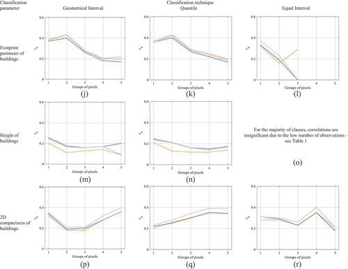
Figure 1c. (continued).

There also exist two cases where the ‘NTL – footprint area’ association (blue lines in Figure 1) emerges the strongest. The first case describes sites with high building density – exceeding 268 buildings per pixel (Figure 1(c)). The second one refers to sites with extremely tall buildings – on average taller than 51 m (Figure 1(m)).

Although the ‘NTL – lateral surface area’ and ‘NTL – footprint area’ associations appeared superior quite infrequently (see Table 2, and also Figure SA1 in the Appendix summarizing the percentages of advantageous associations corresponding to each of the subdivisions reported in Figure 1), such sites may still predominate in some urban areas, making the estimates of the urban extent substantially inaccurate.

3.2. Potential inaccuracies of NTL-Based estimates of urban extent

The obtained results have important applied meaning in the research aimed at estimating urban extent via NTLs. Thus, the urban extent of sites hosting large footprint-size buildings may be estimated inaccurately if measured via the buildings’ total footprint area or total volume. The inaccurate estimation may also occur if sites with remotely located buildings are analysed via the buildings’ total footprint area or total volume. Similarly, inaccuracies in the urban extent estimates are expected for sites with high buildings density or tall buildings if total volume or lateral surface are used as measures instead of footprint area.

Table 3 reports bivariate linear models for the association between the log-transformed urban extent measures (either total surface area, volume, or footprint area of the buildings) and the log-transformed NTLs for some potentially problematic groups of pixels: namely, those with the largest, most remotely located, the tallest buildings, or the highest number of buildings per pixel. The cells with the most accurate estimates are marked grey. As can be derived from the table, for sites hosting the largest buildings (with a footprint area ≥ 7,285 m²), a 1% increase in NTLs corresponds to the 0.32% increase in urban extent if the latter is estimated via the total lateral surface area – the most appropriate measure for such sites. In the meantime, if measured via the total volume or the total footprint area, the increase appears lower − 0.22% and 0.05% respectively, implying a 1.5–6.4-fold underestimation. Similarly, for sites hosting the most remotely located buildings (with the average distance between the two neighbouring buildings ≥ 7.2·10⁻⁴ dd), usage of an inappropriate measure – either the total volume or the total footprint area – may result in 1.1–1.5-fold underestimation of the urban extent (0.21–0.27% instead of the more accurate estimation of 0.31% increase). For sites hosting the highest number of buildings and sites hosting the tallest buildings, underestimation of the urban extent may reach 1.1 and 1.6-fold, respectively, if not measured via the total footprint area.

Table 3. Linear bivariate regressions for estimation of urban extent via NTL intensities (Note: The most accurate estimates are marked grey).

Explanatory variable	Dependent variables – Urban extent proxies:
	Lateral surface area (m^2, lg)		Volume (m^3, lg)		Footprint area (m^2, lg)
	Beta	t	Beta	t	Beta	t
(i) Sites hosting the largest buildings (average footprint area ≥ 7,285 m^2; N = 163*)
NTLs (10^−9 W cm^−2 sr^−1, lg)	0.315	(4.214)***	0.216	(2.802)***	0.049	(0.620)
(ii) Sites hosting the largest buildings (average footprint perimeter ≥560 m; N = 95*)
NTLs (10^−9 W cm^−2 sr^−1, lg)	0.320	(3.255)***	0.174	(1.702)*	−0.012	(−0.119)
(iii) Sites hosting the most remotely located buildings (average distance ≥ 7.2·10^-4 dd; N = 317*)
NTLs (10^−9 W cm^−2 sr^−1, lg)	0.307	(5,718)***	0.270	(4.971)***	0.205	(3.714)***
(iv) Sites with the highest buildings’ density (n. of buildings per pixel ≥ 268; N = 702*)
NTLs (10^−9 W cm^−2 sr^−1, lg)	0.705	(26.326)***	0.767	(31.686)***	0.768	(31.755)***
(v) Sites hosting the tallest buildings (average height ≥51 m; N = 21*)
NTLs (10^−9 W cm^−2 sr^−1, lg)	0.194	(0.885)	0.191	(0.868)	0.298	(1.394)

* See Table 2.

3.3. Analysis of entire cities

Table 4 reports the correlations between NTLs and the three examined urban extent measures for each of the 38 cities. As can be seen from the table, for the overwhelming majority of the cities, the highest correlation is observed between NTLs and the total volumes of the hosted buildings. Only for five European capitals – Bucharest, Lisbon, Riga, Skopje, and Valetta – NTLs stronger correlate with the total lateral surface area of the buildings. The NTLs’ correlation with the total footprint area never emerged as superior, presumably due to the lack of sites with either tall or densely located buildings in the studied cities.

Table 4. Kendall’s tau-b correlations of NTLs with three measures of urban extent by cities.

City	Number of pixels under consideration	Correlations of NTLs with urban extent measures:
		Total footprint area (m^2)	Total lateral surface area (m^2)	Total volume (m^3)
Amsterdam	570	0.296	0.209	0.354
Ankara	702	0.319	0.316	0.337
Athens	705	0.198	0.179	0.237
Beograd	565	0.363	0.429	0.493
Berlin	589	0.149	0.060	0.217
Bern	441	0.578	0.540	0.581
Bratislava	504	0.252	0.264	0.312
Brussels	625	0.395	0.357	0.460
Bucharest	648	0.359	0.404	0.403
Budapest	648	0.285	0.301	0.393
Copenhagen	529	0.428	0.441	0.488
Dublin	568	0.459	0.380	0.519
Helsinki	1491	0.344	0.314	0.407
Leucosis	355	0.321	0.332	0.358
Lisbon	608	0.392	0.457	0.437
Ljubljana	475	0.515	0.481	0.566
London	675	0.399	0.382	0.448
Luxembourg	283	0.508	0.510	0.536
Madrid	680	0.338	0.372	0.372
Oslo	1243	0.401	0.347	0.439
Paris	672	0.101	0.026	0.124
Podgorica	293	0.508	0.501	0.565
Praha	616	0.351	0.346	0.394
Pristina	286	0.581	0.540	0.596
Reykjavik	794	0.440	0.402	0.464
Riga	472	0.185	0.254	0.237
Roma	724	0.489	0.491	0.513
Sarajevo	538	0.535	0.529	0.584
Skopje	377	0.485	0.543	0.520
Sofia	656	0.345	0.411	0.448
Stockholm	1462	0.426	0.408	0.471
Tallinn	786	0.434	0.434	0.486
Tirana	453	0.482	0.480	0.504
Valetta	409	0.402	0.441	0.437
Vilnius	499	0.536	0.541	0.580
Warsaw	566	0.413	0.420	0.450
Wien	595	0.246	0.235	0.341
Zagreb	588	0.501	0.509	0.586
Total	23,690	0.325	0.320	0.366

Table 5 summarizes the comparison of the two groups of cities: (i) those in which NTLs stronger correlate with the lateral surface area vs. (ii) those in which NTLs stronger correlate with the buildings’ volume. The average levels of the built-up environment characteristics in the two groups are compared using the independent samples t-test. As can be seen from the table, the two groups significantly differ (with p < 0.013) in terms of the hosted buildings’ average footprint area (346.82 m² for the cities with stronger ‘NTL – volume’ association vs. 577.29 m² for the cities with stronger ‘NTL – lateral surface area’ association) and perimeter (74.07 m for the cities with stronger ‘NTL – volume’ association vs. 94.02 m for the cities with stronger ‘NTL – lateral surface’ association). This result provides a city-level confirmation for the previously obtained finding – that the stronger ‘NTL – lateral surface area’ association holds for the sites hosting buildings with large footprints (see Figures 1(g,i) in Subsection 3.1).

Table 5. Independent samples t-test for the mean differences of the built-up environment characteristics for the two groups of cities.

Built-up environment characteristics	Mean for the cities with a stronger association between NTL and:		t-stat.	Sig.
	Total volume of buildings (N = 33)	Total lateral surface area of buildings (N = 5)
Average number of buildings per pixel	62.30	35.40	1.320	0.195
Average distance between the neighbouring buildings (dd)	4.03·10^−5	6.03·10^−5	−1.459	0.153
Average footprint area of buildings (m^2)	346.82	577.29	−3.809	0.001
Average footprint perimeter of buildings (m)	74.07	94.02	−2.601	0.013
Average height of buildings (m)	10.91	11.55	−0.632	0.542
Average 2D compactness of buildings (ratio)	0.83	0.81	0.572	0.571
Average 3D compactness of buildings (ratio)	0.84	0.81	1.344	0.187

The difference between the groups was close to significant (p = 0.153) also in terms of the average proximity to the neighbouring building (4.03·10⁻⁵ dd for the cities with stronger ‘NTL – volume’ association vs. 6.03·10⁻³ dd for the cities with stronger ‘NTL – lateral surface area’ association). This city-level finding corroborates with a similar result of the group-level analysis (see Figures 1(d,f) in Subsection 3.1).

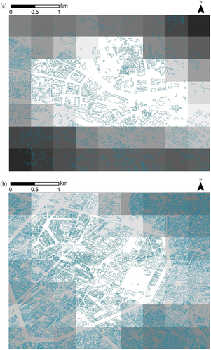
Figure 2 depicts the central areas of two cities: one with relatively large and sparsely located buildings, representing cities with stronger ‘NTL – lateral surface area’ association – see figure 2(a)) vs. another with relatively small and densely located buildings, representing cities with stronger ‘NTL – volume’ association – see Figure 2(b)).

Figure 2. Footprints of buildings (turquoise polygons) in two European city centres overlapped with NTL data (grey-scale raster layers): The centre of Skopje (a) represents cities with a relatively larger in their footprint size and rarely located buildings – in the cities of this type, ‘NTL – lateral surface area’ correlation is stronger. The centre of Brussels (b) represents cities with a relatively smaller size and more densely located buildings – in cities of this type, the ‘NTL – volume’ correlation emerges stronger.

4. Discussion

The present study compares three urban extent measures – the total footprint area, volume, and lateral surface area of the buildings hosted in the central areas of 38 European capital cities, with VIIRS/DNB VNL V2 data on NTLs, emitted from the corresponding areas. Within the study area, NTLs positively correlate with all three examined measures. The main finding of the present analysis is differentiating between the sites characterized by different built-up environments and choosing the most appropriate urban extent measure for each of them. Thus, the association between NTLs and the total footprint area of the buildings emerges as the strongest for the sites with very tall and densely located buildings. The correlation between NTLs and the total volume of the buildings appears the strongest for the sites hosting relatively small in their footprint size and closely located buildings. In the meantime, for the sites hosting the largest and distantly located buildings, NTLs are better associated with the total lateral surface area of the buildings. The explanation for the obtained results might be the following. In large buildings, the area of windows (which are actually the genuine source of light) is closer to the buildings’ lateral surface area than to either their footprint area or volume. Concurrently, in the sites with short distances between the buildings, the light is partially absorbed by neighbouring buildings, making the lateral surface area a less appropriate urban extent measure compared to volume. Furthermore, as the buildings’ density grows, even the volume becomes disadvantageous, giving way to the simplest urban extent proxy – buildings’ footprint area.

The reported findings are practically important for assessing urban extent from NTLs. On the one hand, the analysis performed on a vast variety of non-homogenous urban sites does confirm that the ‘NTL – volume’ association appears superior in most of the cases. This measure is easy to assess: one should multiply areas of residential pixels from a land use raster of sufficiently fine resolution by the elevations of the corresponding areas (obtained from the subtraction of digital surface from digital elevation model raster layers, which are also available globally at a fine spatial resolution (EORC 2023). For this reason, the total volume is a much more convenient urban extent measure than the total lateral surface area. On the other hand, our analysis has revealed certain sites for which total volume does not suit well, which includes sites with high building density, tall, large in footprint size, and distantly located buildings. Sites of these types are rather infrequent (in the study area, out of 23,690 observations, there were only 163 cases with the largest on average footprint area (≥7,285 m²), 317 cases with the most distantly located buildings (≥7.2·10⁻⁴ dd), 702 cases with the highest buildings’ density (≥268 buildings per ~0.25 km²), and 21 cases with the tallest buildings (≥51 metres)). However, they may prevail in some cities. In this case, if the NTL-based assessment of urban extent relies on the total volume of the buildings, the results will be substantially underestimated (up to ~ 1.5 times – see Subsection 3.2). The present analysis thus suggests performing a preliminary estimation of the built-up environment across the study area. If the latter contains enough sites with sufficiently high building density or sufficiently large, tall, or remotely located buildings, then the ‘default’ volume-based estimates should be corrected.

We foresee several directions for further investigation. First, the generality of the obtained results should be evaluated. For example, Shi with co-authors examined another dataset − 25 UK cities treated as the observation units and reported high (up to 0.955) Pearson’s correlations between NTL and the buildings’ footprint area and volume (L. Shi et al. 2020). Our analysis indicates more modest values: upon the aggregation of the data to a city level (with 38 observations, each representing total lights within a city vs. total footprint area/volume/lateral surface area of the buildings hosted by the corresponding city), the Pearson’s correlations of log-transformed NTLs with logs of any of the urban extent measures do not exceed 0.713. Such a discrepancy probably arises from a higher heterogeneity of the European capitals (compared to the cities located in one country) in terms of NTL policies and should be further explored. Second, the dataset might be split into classes based on combinations of different built-up characteristics. This should lead to a more accurate defining the cases requiring a certain urban extent measure. Third, the performed analysis covered only ~ 20×10 km rectangular areas within the cores of the European capitals, due to limited data availability for some cities and our willingness to obtain comparable datasets for all cities. To strengthen the inference, the procedure might be expanded to the whole areas of the capitals, as well as other, non-capital cities. Finally, lights from roads might also be accounted for, which would increase the correlation values, especially for urban sites hosting relatively large and distantly located buildings.

Acknowledgment

The authors thank the University of Haifa for providing the open access funding.

Disclosure statement

No potential conflict of interest was reported by the author(s).

Data availability statement

The data that support the findings of this study are available on request from the corresponding author, NR, upon reasonable request.

Supplementary material

Supplemental data for this article can be accessed online at https://doi.org/10.1080/01431161.2023.2227319.

References

- Doll, C. N. H., J. P. Muller, and C. D. Elvidge. 2000. “Night-Time Imagery as a Tool for Global Mapping of Socioeconomic Parameters and Greenhouse Gas Emissions.” AMBIO: A Journal of the Human Environment 29 (3): 157–162. https://doi.org/10.1579/0044-7447-29.3.157.
- Dou, Y., Z. Liu, C. He, and H. Yue. 2017. “Urban Land Extraction Using VIIRS Nighttime Light Data: An Evaluation of Three Popular Methods.” Remote Sensing 9 (2): 175. https://doi.org/10.3390/rs9020175.
- Ebener, S., C. Murray, A. Tandon, and C. D. Elvidge. 2005. “From Wealth to Health: Modelling the Distribution of Income per Capita at the Sub-National Level Using Night-Time Light Imagery.” International Journal of Health Geographics 4:5. https://doi.org/10.1186/1476-072X-4-5.
- EEA. 2023a. “Urban Atlas.” Accessed January 4, 2023. https://land.copernicus.eu/local/urban-atlas.
- EEA. 2023b. “Building Height 2012.” Accessed May 2, 2023. https://land.copernicus.eu/local/urban-atlas/building-height-2012?tab=metadata.
- Elvidge, C. D., K. E. Baugh, E. A. Kihn, H. W. Kroehl, E. R. Davis, and C. W. Davis. 1997. “Relation Between Satellite Observed Visible-Near Infrared Emissions, Population, Economic Activity and Electric Power Consumption.” International Journal of Remote Sensing 18 (6): 1373–1379. https://doi.org/10.1080/014311697218485.
- EOG. 2023. “VIIRS Nighttime Light.” Accessed January 4, 2023. https://eogdata.mines.edu/products/vnl/.
- EORC. 2023. “ALOS Research and Application Project.” Accessed January 26, 2023. https://www.eorc.jaxa.jp/ALOS/en/urlchangeinfoe.htm.
- ESRI. 2021. “ArcGis Desktop | Desktop GIS Software Suite - Esri.” Accessed November 2, 2023. https://www.esri.com/en-us/arcgis/products/arcgis-desktop/overview.
- ESRI. 2023. “About the Geometrical Interval Classification Method.” Accessed January 11, 2023. https://www.esri.com/arcgis-blog/products/product/mapping/about-the-geometrical-interval-classification-method/.
- Henderson, M., E. T. Yeh, P. Gong, C. D. Elvidge, and K. Baugh. 2003. “Validation of Urban Boundaries Derived from Global Night-Time Satellite Imagery.” International Journal of Remote Sensing 24 (3): 595–609. https://doi.org/10.1080/01431160304982.
- He, C., P. Shi, J. Li, J. Chen, Y. Pan, J. Li, L. Zhuo, and I. Toshiaki. 2006. “Restoring Urbanization Process in China in the 1990s by Using Non-Radiance-Calibrated DMSP/OLS Nighttime Light Imagery and Statistical Data.” Chinese Science Bulletin 51 (13): 1614–1620. https://doi.org/10.1007/s11434-006-2006-3.
- Hopkins, G. R., K. J. Gaston, M. E. Visser, M. A. Elgar, and T. M. Jones. 2018. “Artificial Light at Night as a Driver of Evolution Across Urban-Rural Landscapes.” Frontiers in Ecology and the Environment 16 (8): 472–479. https://doi.org/10.1002/fee.1828.
- IBM. 2020. “SPSS Software.” Accessed March 17, 2020. https://www.ibm.com/analytics/spss-statistics-software.
- Imhoff, M. L., W. T. Lawrence, D. C. Stutzer, and C. D. Elvidge. 1997. “A Technique for Using Composite DMSP/OLS ‘City Lights’ Satellite Data to Map Urban Area.” Remote Sensing of Environment 61 (3): 361–370. https://doi.org/10.1016/S0034-4257(97)00046-1.
- Liu, Z., C. He, Q. Zhang, Q. Huang, and Y. Yang. 2012. “Extracting the Dynamics of Urban Expansion in China Using DMSP-OLS Nighttime Light Data from 1992 to 2008.” Landscape and Urban Planning 106 (1): 62–72. https://doi.org/10.1016/j.landurbplan.2012.02.013.
- Marshall, S., Y. Gong, and N. Green. 2019. “Urban Compactness: New Geometric Interpretations and Indicators.” The Mathematics of Urban Morphology 431–456. https://doi.org/10.1007/978-3-030-12381-9_19/COVER.
- MathWorks. 2021. “MATLAB & Simulink.” Accessed September 11, 2021. https://www.mathworks.com/products/matlab.html.
- Ma, T., C. Zhou, T. Pei, S. Haynie, and J. Fan. 2012. “Quantitative Estimation of Urbanization Dynamics Using Time Series of DMSP/OLS Nighttime Light Data: A Comparative Case Study from China’s Cities.” Remote Sensing of Environment 124:99–107. https://doi.org/10.1016/j.rse.2012.04.018.
- Mellander, C., J. Lobo, K. Stolarick, Z. Matheson, and G. J.-P. Schumann. 2015. “Night-Time Light Data: A Good Proxy Measure for Economic Activity?” PloS One 10 (10): e0139779. https://doi.org/10.1371/journal.pone.0139779.
- Montero, R. S., and E. Bribiesca. 2009. “State of the Art of Compactness and Circularity Measures.” International Mathematical Forum 4 (27): 1305–1335.
- Rybnikova, N., B. A. Portnov, I. Charney, and S. Rybnikov. 2021. “Delineating Functional Urban Areas Using a Multi-Step Analysis of Artificial Light-At-Night Data.” Remote Sensing 13:3714. https://doi.org/10.3390/RS13183714.
- Shi, L., G. M. Foody, D. S. Boyd, R. Girindran, L. Wang, Y. Du, and F. Ling. 2020. “Night-Time Lights are More Strongly Related to Urban Building Volume Than to Urban Area.” Remote Sensing Letters 11 (1): 29–36. https://doi.org/10.1080/2150704X.2019.1682709.
- Shi, K., C. Huang, B. Yu, B. Yin, Y. Huang, and J. Wu. 2014. “Evaluation of NPP-VIIRS Night-Time Light Composite Data for Extracting Built-Up Urban Areas.” Remote Sensing Letters 5 (4): 358–366. https://doi.org/10.1080/2150704X.2014.905728.
- Tay, K. 2023. “Spearman’s Rho and Kendall’s Tau.” Accessed January 8, 2023. https://statisticaloddsandends.wordpress.com/2019/07/08/spearmans-rho-and-kendalls-tau/.