Rejection methods for vegetation mapping using hyperspectral airborne data

ABSTRACT

Vegetation mapping from remote sensing data has proven useful for monitoring ecosystems at local, regional and global scales. Generally based on supervised classification methods, ecosystem mapping needs representative and consistent labelling. Such completeness is often difficult to achieve and requires the exclusion of minority species poorly represented in the studied scene in the training base. This exclusion leads to wrong predictions in the resulting map. In this study, the use of a posteriori classification rejection methods to limit the errors associated with minority species was evaluated in three different mapping scenarios: classification according to vegetation layers, prediction of genera from various vegetation types from low vegetation to trees and mapping of habitat (assemblages of species). For this purpose, several supervised classification methods based on Support Vector Machines (SVM), Random Forests (RF) and Regularized Logistic Regression (RLR) algorithms were first applied to hyperspectral images covering the reflective domain. On these classifications, the usual evaluation methods (confusion matrix and its derivatives calculated on an independent test set composed of the majority species) showed performances similar to those of the state-of-the-art. However, the introduction of a new score taking into account minority species demonstrated the need to include them in the evaluation process to provide robust performance quantification representing map effectiveness. Three a posteriori rejection methods, based on simple thresholding, K-means and SVM algorithms, were well suited to monitor minority species. The performance gain depended on the mapping scenario, the machine learning model and the rejection method. An increase in performance with the inclusion of minority species of up to 12% could be observed through the new score. These methods also detected a similar proportion of prediction errors associated with predominant species

KEYWORDS:

• Supervised classification
• rejection method
• hyperspectral
• vegetation mapping
• machine learning, minority species

1. Introduction

Biodiversity and vegetation play a crucial role in regulating the impacts of human activities on the environment (IPBES 2019). Indeed, both are involved in carbon cycle and climate change mitigation (Grace, Mitchard, and Gloor 2014; IPBES 2019), soil erosion and conservation, contamination transfer preservation (Kafle et al. 2022) and other major ecosystem services (Mori, Lertzman, and Gustafsson 2017). The characterization of plant ecosystems through health status, biomass, plant species or functional traits (Qiu et al. 2020; Faucon, Houben, and Lambers 2017) and their monitoring are important to analyse their roles.

Optical remote sensing plays a key role in mapping and monitoring vegetation, particularly concerning species distribution and diversity (Cavender-Bares et al. 2022; Skidmore et al. 2021). By using airborne or spaceborne passive optical instruments, remote sensing can provide detailed spectral and phenological information on vegetation cover across large areas, cost-effectively. Supervised classification techniques have proven to be powerful for exploiting remote sensing data to map and monitor vegetation properties (Cavender-Bares et al. 2022). Such techniques allow the automatic identification of latent features in the data and the classification of images’ pixels into different vegetation types, habitats or species (Fassnacht et al. 2016; Kluczek, Zagajewski, and Zwijacz-Kozica 2023), or according to the plants’ functional traits (Asner et al. 2015; Jachowski et al. 2013; Pham et al. 2019). A large number of studies have demonstrated the efficiency of hyperspectral remote sensing images to map vegetation cover and species (Fabian Ewald Fassnacht et al. 2016; Wang and Gamon 2019). However, as highlighted in (Fabian E. Fassnacht et al. 2014), very few studies have addressed the robustness of classification approaches in different contexts.

Supervised classification requires a selection of labelled pixels, built, for example, owing to ground-level inventories, to both train the selected machine learning algorithm and evaluate its2019 performance. Vegetation classification of a whole scene requires an exhaustive species inventory which is difficult to achieve because of the necessary human means, the presence of inaccessible areas and the low representativeness of specific species. The training and testing sets used by supervised classification are then not completely representative of the vegetation in the observed scene. Only the dominant communities and/or species are then often considered (Kluczek, Zagajewski, and Kycko 2022; Kluczek, Zagajewski, and Zwijacz-Kozica 2023; Marcinkowska-Ochtyra et al. 2017). The resulting maps and scores are therefore biased towards the dominant classes. In addition, the presence of mixed pixels, representing an area with more than one species, is inherent in remote sensing image processing (Petrou 1999). Their abundance depends on the ratio between the vegetated patch sizes and the spatial resolution of the remote sensing devices. Further mixed pixels are located at the edges of homogeneous areas. These mixed pixels are often not represented in the training and testing sets usually based on pure classes, composed of a single species. This lack of completeness in the training set leads to incorrect predictions (Kluczek, Zagajewski, and Zwijacz-Kozica 2023; Petrou 1999). Similarly, their non-inclusion in the testing set positively biases the performance related to the resulting classification map. To reduce these errors, it is crucial to assign the non-inventoried species and mixed pixels to a rejection class grouping pixels potentially misclassified. It is also essential to consider these outliers when assessing the produced map quality to reduce these positive biases.

Various problems related to the scenario of learning with a rejection option have been studied in the past (Cortes, DeSalvo, and Mohri 2016). The rejection class processing was introduced in two ways: (i) a posteriori to the classification algorithm by exploiting the classified results and (ii) directly integrated into the classifier scheme where the learner is given the option to reject an instance instead of predicting its class. A reject option in classification was first considered by Chow (1970). The proposed reject option was based on the Bayes rule and consisted in not classifying a datapoint if the maximum post-classification component of the probability vector was lower than a given threshold. Later, optimal rejection rules based on the Receiver Operating Characteristic (ROC) curve and a subset of the training data were proposed (Santos-Pereira and Pires 2005). The approaches which simultaneously trained a classifier and a rejector had theoretical justification in the binary case and most of them did not apply directly to multiclass cases (Charoenphakdee et al. 2020; Cortes, DeSalvo, and Mohri 2016; Ni et al. 2019). Multiple other specifications for embedding a reject option into the classification process existed through new risk minimization approaches or cost functions and some were specific to Support Vector Machines (SVM) or Deep Neural Networks (DNN) (Condessa, Bioucas-Dias, and Kovačević 2017; Grandvalet et al. 2011; Laroui et al. 2021; Wegkamp and Yuan 2011; Yuan and Wegkamp 2010). These specifications were optimized using a training set. For instance, Charoenphakdee et al. proposed a cost-sensitive approach to classification with rejection avoiding class-posterior probability estimation and having a flexible choice of loss functions (Charoenphakdee et al. 2020). Nevertheless, the majority of studies rejecting samples in the classifier design addressed applications on reduced data sets, and even fewer handled remote sensing data, known to be voluminous. For example, deep learning methods are known to be computationally expensive and memory-intensive methods that require a large training database (Paoletti et al. 2019). While such methods seem promising, their prerequisites make them difficult to use in a wide range of context (in particular for small data sets, reduced-size scene).

As part of studies based on remote sensing, Condessa et al. specified two classification methods with rejection using contextual (spatial) information in the field of hyperspectral images (Condessa et al. 2015; Condessa, Bioucas-Dias, and Kovacevic 2015). One was embedded within the classification by an extra class (joint computation of context and rejection), while the other was carried out a posteriori (sequential computations of context and rejection). These two methods were compared on a vegetation scene, the AVIRIS Indian Pines scene, composed of and containing two-thirds agriculture and one-third forest or other natural perennial vegetation. The performance improvements resulting from the combination of rejection and context were more significant for classifiers with lower performance. By classifying with rejection, gains were equivalent to increasing twice the training set size. However, these promising methods tested on small scenes (145 × 145 pixels with 200 spectral bands and 610 × 340 pixels with 103 spectral bands) may be limited and much less effective on scenes of larger sizes owing to their computational expensive cost.

Concerning the a posteriori integration of the prediction class without using context, the way to determine uncertain predictions consisted of using thresholds on the prediction probabilities (Aval 2016; Gimenez et al. 2022). Gimenez et al. proposed to detect misclassified pixels using an a posteriori rejection class incorporated in a majority vote. This rule proved especially suited to handle large volume hyperspectral data in species classification applications. However, it was based on empirically established thresholds specific to the observed scene. Easy-to-use and standard methods such as SVM and K-means could be applied to segment spaces such as those resulting from the probabilities associated with a classification (Ahmed, Basu, and Kumaravel 2013; Djeffal 2012; Grandvalet et al. 2011). The biggest advantages provided by such methods lie in their ability to detect errors without changing predictions, without the need for the initial multispectral or hyperspectral data, and the development of specific algorithms.

To our knowledge, no remote sensing studies have evaluated their potential to detect outliers for vegetation mapping purposes, as done by Huang, Boom, and Fisher (2015) for fish species based on video classification. In a more general way, very few a posteriori rejection methods have been developed in the field of hyperspectral and multispectral images.

This study aims to propose and compare three a posteriori rejection methods to limit classification errors and to detect minor species and mixed pixels in three vegetation mapping contexts (genera mapping, discrimination of vegetation layers and cover species mapping). The study is organized as follows. First, in Section 2, the three scenarios, defined by three different sites, field surveys and hyperspectral data, are introduced. Supervised classification and rejection techniques considered are then detailed. In Section 3, the results of supervised classification techniques without rejection monitoring are first presented and compared before describing the rejection results for the different scenarios. The fourth section discusses these results. Conclusions and perspectives are finally given in Section 5.

2. Materials and methods

2.1. Study sites

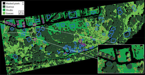
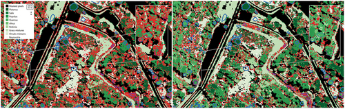
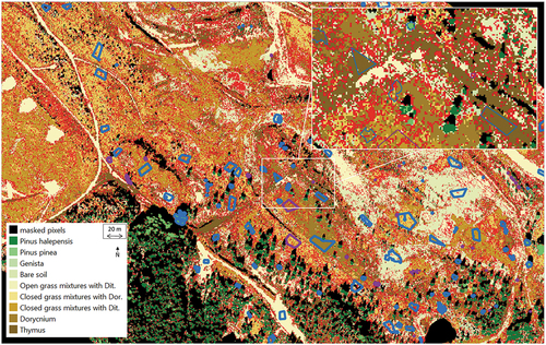
Three sites located in a temperate region with different species diversity were selected for this study. The first site, called site 1 next, is part of the riparian forest located in Fauga-Mauzac. The site covers about 12 ha and the majority of trees are pubescent oaks. The second site, site 2, extending over 245 ha, includes riparian and planted forests, shrubby and grassland vegetation heterogeneously distributed, and agricultural land (Gimenez et al. 2022). The last site, noted as site 3, is a former ore processing site and the studied area covers approximately 120 ha (Fabre et al. 2020). The vegetation is composed of developing trees (pines, poplars) distributed in various patches of forestry, woodland, single tree rows and closed and open lawns (vegetation cover varies between 10% and 70%) with species present in the Mediterranean region (e.g. Aphyllanthes monspeliensis, Bituminaria bituminosa, Dittrichia viscosa, Pallenis spinosa, Plantago lanceolata, Spanish brooms).

2.2. Data

2.2.1. Hyperspectral images

The images were hyperspectral data covering the reflective spectral domain (400–2500 nm). Atmospheric and geometric corrections were applied to images and orthorectified spectral reflectances were processed in this study (Gimenez et al. 2022). Due to the low signal-to-noise ratio (SNR), the spectral bands with atmospheric transmission below 80% were not retained, as described in (Erudel et al. 2017). A Savitzky-Golay smoothing filter (spectral window length of 11 bands and third-degree polynomial) was also applied to the spectral dimension. The image characteristics for each site are described in Table 1.

Table 1. Hyperspectral image characteristics. Spectral band number provided after atmospheric absorption band filtering.

Site	Instrument	Spatial resolution (m)	Spectral band number	Scene size (in pixels)
Site 1	AISA FENIX-1K	0.75	232	825 × 426
Site 2	HySpex	1	221	2473 × 2516
Site 3	AISA FENIX-1K	0.75	232	4145 × 3814

2.2.2. Species inventory

Species inventories were conducted in-field from 2020 to 2022 to identify the predominant genera and species of each site. Units, which corresponded to individual tree crowns, mono-species or genus areas for homogeneous regions at the metric spatial resolution, or species assemblages for herbaceous plants or shrubs were recorded using a GPS-RTK with a centimetre precision (Table 2). The species inventory was divided into two categories for each site:

• Units related to predominant species or genera, identified in bold in Table 2, were used as classes for the supervised classification step (see Section 2.3.1) and to evaluate the rejection methods (see Section 2.3.2),

• Minor species or genera were retained to evaluate the rejection methods only (see Section 2.3.2).

Table 2. Species Inventories for each site. Species in bold were those defining classes for supervised classification purposes.

Vegetation layer	Site 1	Site 2	Site 3
Tree layer	Quercus (6472 pixels) Tilia (441 pixels) Juglans (191 pixels) Morus (223 pixels) Ulmus (22 pixels) Robinia (206 pixels) Fraxinus (16 pixels) Prunus (56 pixels)	Platanus (4183 pixels) Salix (1521 pixels) Populus (2565 pixels) Quercus (2936 pixels) Fraxinus (931 pixels) Acer (403 pixels) Alnus (1588 pixels) Ulmus (305 pixels) Robinia (1536 pixels) Castanea (107 pixels) Juglans (388 pixels) Corylus (40 pixels)	Pinus halepensis (718 pixels) Pinus pinea (1444 pixels) Populus (554 pixels) Quercus ilex (564 pixels) Quercus robur (156 pixels) Alnus (47 pixels)
Shrub layer	Shrubs mixtures (Cornus, Crataegus, Rubus)(1834 pixels)	Reynoutria japonica (1533 pixels) Shrubs mixtures with Rubus fruticosus (2015 pixels) Zea mais (4316 pixels)	Genista (1208 pixels)
Herbaceous layer	Closed grass mixtures (4353 pixels)	Closed grass mixtures (3123 pixels)	Open grass mixtures with Dittichia viscosa (2121 pixels) Closed grass mixtures with Dorycnium and dicots (2161 pixels) Closed grass mixtures with Dittichia viscosa and Brachypodus retusum (2303 pixels) Dorycnium (1766 pixels) Thymus (963 pixels)

The specificity of each site made it possible to define three different vegetation classification scenarios. The scenario associated with the first site represented a vegetation layer classification (one class per layer or stratum defined according to the height of the ground cover). Site 2 application was related to genera classification without overlapping classes (one genus or species corresponded strictly to one class, from low vegetation to trees). The scenario linked to site 3 was associated with a habitat classification with overlapping classes (assemblages of species, one species can be in several classes defined according to its proportion). For site 3 with lots of sparse vegetation, a further class corresponding to bare soil completed the species inventory (1236 pixels).

2.3. Methods

After a preprocessing stage of the hyperspectral images, a commonly used supervised classification procedure based on usual machine learning models in literature was retained (Section 2.3.1). The resulting classification maps of each site which did not integrate the rejection class were then used as reference maps to compare the different rejection methods, described in Section 2.3.2.

2.3.1. Preprocessing

For each image, pixels corresponding to shadow or non-studied land-use classes (i.e. water, buildings, etc.) were located and removed manually or automatically by specific thresholded spectral indices as described in detail in (Fabre et al. 2020; Gimenez et al. 2022). The spectral features of the remaining pixels were then standardized.

2.3.2. Supervised classification procedure

Training and testing sets were created with a simple data-splitting procedure. Fifty per cent of the labelled units were randomly selected for training, while the 50% left were used for the classification evaluation stage (Fassnacht et al. 2016). This led to an unbalanced number of samples per class within the training and testing sets (see Table 2).

Five classification models commonly used in the literature to process hyperspectral and multispectral images, Random Forest (RF) (Breiman 2021), Support Vector Machines (SVM) with linear and Radial Base Function kernels (RBF) (Vladimir 1998) and Regularized Logistic Regression (RLR) with ℓ1 and ℓ2 regularizations (Pant et al. 2014), were processed using Python’s scikit learn package (version 1.0.2) (Pedregosa et al. 2012). The introduction of these five models allowed verifying if performance improvements resulting from the rejection class integration depended on the chosen classification model (Condessa, Bioucas-Dias, and Kovacevic 2015).

Hyperparameters were chosen using 10-fold cross-validation across the training set. Performance assessment before rejection was finally made using visual analysis of the resulting maps and metrics derived from the confusion matrix calculated on the testing set. In particular, the Overall Accuracy (OA), defined as the number of correctly predicted pixels divided by the total of pixels to predict, and the F1-score, a class-wise performance indicator which, unlike the OA, is not biased by the number of representatives of the considered classes, were used to analyse classifications (Gimenez et al. 2022; Lu and Weng 2007). Since these metrics only considered predominant classes, a new score, named True accuracy (TA), defined as the overall accuracy extended to reference data non-considered for classification owing to the small sample number (minor classes), was introduced:

(1) $\mathrm{T}\mathrm{A}=\frac{\mathrm{w}\mathrm{e}\mathrm{l}\mathrm{l}-\mathrm{c}\mathrm{l}\mathrm{a}\mathrm{s}\mathrm{s}\mathrm{i}\mathrm{f}\mathrm{i}\mathrm{e}\mathrm{d}}{\left(\mathrm{p}\mathrm{r}\mathrm{e}\mathrm{d}\mathrm{o}\mathrm{m}\mathrm{i}\mathrm{n}\mathrm{a}\mathrm{n}\mathrm{t}\mathrm{c}\mathrm{l}\mathrm{a}\mathrm{s}\mathrm{s}\mathrm{e}\mathrm{s}\right)\cup \left(\mathrm{m}\mathrm{i}\mathrm{n}\mathrm{o}\mathrm{r}\mathrm{c}\mathrm{l}\mathrm{a}\mathrm{s}\mathrm{s}\mathrm{e}\mathrm{s}\right)\hspace{0.17em}}$(1)

2.3.3. Rejection methods

Different rejection methods were considered to perform a posteriori rejection. All these methods were based on rejection rules (described below). These rules, derived from probabilities linked to classification predictions, aimed to determine which pixels should be rejected or not and were used differently by the proposed rejection methods. Two clustering-based rejection methods described next were compared to a simple thresholding method, related to Chow’s rule, and considered as a reference (Chow 1970). The rejection performance was then calculated using different metrics described below.

Rejection rules: Different rules were defined to a posteriori determine the correctness of the classification for each pixel of the map previously obtained:

1. Minimum probability rule: a pixel was considered as almost surely badly classified if the probability of prediction associated with the predicted class was below a given good classification threshold.

2. Difference probability rule: a pixel was considered as almost surely correctly classified if the probability of prediction was above the given good classification threshold and if the difference between the two highest probabilities was above a confusion threshold within {0; 0.05; 0.1; 0.15; 0.20; 0.25; 0.3}.

The good classification threshold was empirically fixed to 0.5 in both rules. The difference rule with a confusion threshold fixed to 0 is equivalent to the minimum probability rule alone. The rejection methods processed the misclassified pixels according to these decision rules.

Rejection methods: The clustering of probability vectors had already been investigated in several previous works in different scientific domains (Garcia-Garcia, Santos-Rodriguez, and Parrado-Hernandez 2012; Van 2010). Several common algorithms were then applied, such as K-means or SVM (Ahmed, Basu, and Kumaravel 2013; Djeffal 2012; Grandvalet et al. 2011). In our study, two rejection methods applied to probability vectors were implemented through these algorithms. K-means is a common unsupervised partitioning-based algorithm without a priori knowledge of the data labels. SVMs have been successfully applied to various classification areas with great flexibility and a high level of classification accuracy. The use of SVMs for clustering (unsupervised learning) has also been considered in some different ways. These algorithms were implemented to group pixels by similarity, according to their probability vectors, in which each component was the probability to belong to a given species. In this study, K-means and SVM rejection methods were compared to simple probability thresholding considered as the reference method in the following (Aval 2016). The proposed rejection techniques are detailed as follows:

• Rejection by thresholding (reference method): the rules introduced previously were applied to reject pixels.

• K-means rejection: Given the number of clusters, K-means minimizes the distance between the data points and the cluster centroids. Thus, K-means asks for compact and isotropic partitions according to this distance to ensure optimal separations. In the present case, the Wasserstein distance, particularly fit to probability problems (Givens and Shortt 1984), was retained. The number of clusters was defined as the number of classes, the idea being to find the initial classes. Only pixels in agreement with the previous rejection rules were used to perform an initial clustering. A threshold of correctness was then defined within each cluster. The choice to reject or not a pixel that did not follow the rejection rules was finally done by comparing the values obtained by multiplying the chosen threshold with the radius of each cluster (distance between the centroid and the furthest point from the centroid). If the distance to one centroid was inferior to one of these values, the pixel was associated with this cluster and not rejected. The pixel was rejected otherwise.

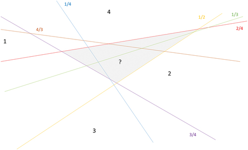
• SVM rejection: SVM supposes that data could be separated by a hyperplane (or decision boundary) with a certain margin (Vladimir Vapnik 1998). In the case of multiple classes, hyperplanes could be derived from two strategies: One-Versus-Rest (OVR) and One-Versus-One (OVO). In our classification problem, (K(K-1)) hyperplanes, with K the number of classes, were optimized (see Figure 1). This method of construction meant that the decision function for an SVM was specified by a subset of the data, called the training set. This set was built with pixels determined as well classified according to the previously defined decision rules. The training stage provided the decision functions which informed how close to the decision boundary a pixel was (close to the boundary was equivalent to a low confidence decision). Rejection was then performed only on pixels considered misclassified according to the decision rules. To make this rejection, the relative difference between the nearest and second-nearest decision function values was analysed. For a given pixel, the rejection was made if this difference in the decision function was inferior to the median or third quartile of these relative differences (Grandvalet et al. 2011). This indicated that the classifier did not decide between the two classes and that the pixel was in an indecision area. The specificity of this algorithm was that a rejection rate was introduced instead of determining a threshold.

Figure 1. Example of an indecision area (in grey) obtained with SVM with an OVO strategy for four classes. Classes are noted in black and corresponding decision hyperplanes are in colour.

Performance assessment: The rejection efficiency was evaluated using the following procedure:

• Visual assessment of the classification map after rejection: For each site, some specific pixel areas like minor species or mixed pixels had to be rejected.

• Labelled data concerning predominant classes (see 2.2.2): errors were quantified by three different metrics adapted from the set of performance measures for the evaluation of classification with rejection proposed in the literature (Guichard, Toselli, and Co 2010; Condessa, Bioucas-Dias, and Kovačević 2017). Not related to minority classes, these metrics indicated whether the choice to reject pixels improved the quality of the classification of predominant classes by removing misclassified pixels.

Non-Rejected Accuracy (NRA):

(2) $\mathrm{N}\mathrm{R}\mathrm{A}=\frac{\left(\mathrm{w}\mathrm{e}\mathrm{l}\mathrm{l}-\mathrm{c}\mathrm{l}\mathrm{a}\mathrm{s}\mathrm{s}\mathrm{i}\mathrm{f}\mathrm{i}\mathrm{e}\mathrm{d}\right)\cap \left(\mathrm{n}\mathrm{o}\mathrm{n}-\mathrm{r}\mathrm{e}\mathrm{j}\mathrm{e}\mathrm{c}\mathrm{t}\mathrm{e}\mathrm{d}\right)}{\left(\mathrm{n}\mathrm{o}\mathrm{n}-\mathrm{r}\mathrm{e}\mathrm{j}\mathrm{e}\mathrm{c}\mathrm{t}\mathrm{e}\mathrm{d}\right)\cap \left(\mathrm{p}\mathrm{r}\mathrm{e}\mathrm{d}\mathrm{o}\mathrm{m}\mathrm{i}\mathrm{n}\mathrm{a}\mathrm{n}\mathrm{t}\mathrm{c}\mathrm{l}\mathrm{a}\mathrm{s}\mathrm{s}\mathrm{e}\mathrm{s}\right)}$(2)

NRA corresponds to the OA after rejection. Indeed, it indicates the percentage of non-rejected pixels from well-classified predominant classes.

Classification quality:

(3) $\mathrm{Q}=\frac{\left(\left(\mathrm{w}\mathrm{e}\mathrm{l}\mathrm{l}-\mathrm{c}\mathrm{l}\mathrm{a}\mathrm{s}\mathrm{s}\mathrm{i}\mathrm{f}\mathrm{i}\mathrm{e}\mathrm{d}\right)\cap \left(\mathrm{n}\mathrm{o}\mathrm{n}-\mathrm{r}\mathrm{e}\mathrm{j}\mathrm{e}\mathrm{c}\mathrm{t}\mathrm{e}\mathrm{d}\right)\right)\cup \left(\left(\mathrm{b}\mathrm{a}\mathrm{d}-\mathrm{c}\mathrm{l}\mathrm{a}\mathrm{s}\mathrm{s}\mathrm{i}\mathrm{f}\mathrm{i}\mathrm{e}\mathrm{d}\right)\cap \left(\mathrm{r}\mathrm{e}\mathrm{j}\mathrm{e}\mathrm{c}\mathrm{t}\mathrm{e}\mathrm{d}\right)\right)}{\left(\mathrm{p}\mathrm{r}\mathrm{e}\mathrm{d}\mathrm{o}\mathrm{m}\mathrm{i}\mathrm{n}\mathrm{a}\mathrm{n}\mathrm{t}\mathrm{c}\mathrm{l}\mathrm{a}\mathrm{s}\mathrm{s}\mathrm{e}\mathrm{s}\right)}$(3)

Classification quality also corresponds to an extension of OA with rejection since both OA and Q are defined as a ratio of good classification over pixels from predominant classes. Nevertheless, in terms of quality, a good classification could be derived from a really good class assignment or an effective rejection linked with a bad class prediction.

Rejection quality:

(4) $\phi =\frac{\frac{\left(\mathrm{b}\mathrm{a}\mathrm{d}-\mathrm{c}\mathrm{l}\mathrm{a}\mathrm{s}\mathrm{s}\mathrm{i}\mathrm{f}\mathrm{i}\mathrm{e}\mathrm{d}\right)\cap \left(\mathrm{r}\mathrm{e}\mathrm{j}\mathrm{e}\mathrm{c}\mathrm{t}\mathrm{e}\mathrm{d}\right)}{\left(\mathrm{w}\mathrm{e}\mathrm{l}\mathrm{l}-\mathrm{c}\mathrm{l}\mathrm{a}\mathrm{s}\mathrm{s}\mathrm{i}\mathrm{f}\mathrm{i}\mathrm{e}\mathrm{d}\right)\cap \left(\mathrm{r}\mathrm{e}\mathrm{j}\mathrm{e}\mathrm{c}\mathrm{t}\mathrm{e}\mathrm{d}\right)}}{\frac{\left(\mathrm{b}\mathrm{a}\mathrm{d}-\mathrm{c}\mathrm{l}\mathrm{a}\mathrm{s}\mathrm{s}\mathrm{i}\mathrm{f}\mathrm{i}\mathrm{e}\mathrm{d}\right)}{\left(\mathrm{w}\mathrm{e}\mathrm{l}\mathrm{l}-\mathrm{c}\mathrm{l}\mathrm{a}\mathrm{s}\mathrm{s}\mathrm{i}\mathrm{f}\mathrm{i}\mathrm{e}\mathrm{d}\right)}}$(4)

This last score allows for the assessment of the ability of the rejection method to reject badly classified pixels and not the well-classified ones.

• Labelled data concerning minor classes were used to evaluate the power of rejection methods to deal with the unconsidered across two new metrics:

  True Non-Rejected Accuracy (TNRA):

  (5) $\mathrm{T}\mathrm{N}\mathrm{R}\mathrm{A}=\frac{\left(\mathrm{w}\mathrm{e}\mathrm{l}\mathrm{l}-\mathrm{c}\mathrm{l}\mathrm{a}\mathrm{s}\mathrm{s}\mathrm{i}\mathrm{f}\mathrm{i}\mathrm{e}\mathrm{d}\right)\cap \left(\mathrm{n}\mathrm{o}\mathrm{n}-\mathrm{r}\mathrm{e}\mathrm{j}\mathrm{e}\mathrm{c}\mathrm{t}\mathrm{e}\mathrm{d}\mathrm{p}\mathrm{i}\mathrm{x}\mathrm{e}\mathrm{l}\mathrm{s}\right)}{\left(\mathrm{n}\mathrm{o}\mathrm{n}-\mathrm{r}\mathrm{e}\mathrm{j}\mathrm{e}\mathrm{c}\mathrm{t}\mathrm{e}\mathrm{d}\right)\hspace{0.17em}}$(5)

As TA is the extension of OA with minority species taken into account, the TNRA is the extension of the NRA. It corresponds to the proportion of non-rejected pixels that are well classified among all the non-rejected ones.

Minor rejection rate:

(6) ${\mathrm{R}}_{\mathrm{\%}\mathrm{m}\mathrm{i}\mathrm{n}}=\frac{\left(\mathrm{r}\mathrm{e}\mathrm{j}\mathrm{e}\mathrm{c}\mathrm{t}\mathrm{e}\mathrm{d}\right)\cap \left(\mathrm{m}\mathrm{i}\mathrm{n}\mathrm{o}\mathrm{r}\mathrm{c}\mathrm{l}\mathrm{a}\mathrm{s}\mathrm{s}\mathrm{e}\mathrm{s}\right)}{\left(\mathrm{m}\mathrm{i}\mathrm{n}\mathrm{o}\mathrm{r}\mathrm{c}\mathrm{l}\mathrm{a}\mathrm{s}\mathrm{s}\mathrm{e}\mathrm{s}\right)}$(6)

The minor rejection rate is the proportion of pixels from minor classes effectively rejected.

This score could be compared to the rejection rate, which is simply the proportion of rejected pixels among labelled data (predominant and minor species):

(7) ${\mathrm{R}}_{\mathrm{\%}}=\frac{\left(\mathrm{r}\mathrm{e}\mathrm{j}\mathrm{e}\mathrm{c}\mathrm{t}\mathrm{e}\mathrm{d}\right)}{\left(\mathrm{m}\mathrm{i}\mathrm{n}\mathrm{o}\mathrm{r}\mathrm{c}\mathrm{l}\mathrm{a}\mathrm{s}\mathrm{s}\mathrm{e}\mathrm{s}\right)\cup \left(\mathrm{p}\mathrm{r}\mathrm{e}\mathrm{d}\mathrm{o}\mathrm{m}\mathrm{i}\mathrm{n}\mathrm{a}\mathrm{n}\mathrm{t}\mathrm{c}\mathrm{l}\mathrm{a}\mathrm{s}\mathrm{s}\mathrm{e}\mathrm{s}\right)}$(7)

3. Results

3.1. Supervised classification

Classification maps obtained for each site and each supervised classification model presented previously were evaluated with the OA and the new TA metrics. Scores are reported in Table 3.

Table 3. Supervised classification performances.

Site	Site 1		Site 2		Site 3
Performances	OA	TA	OA	TA	OA	TA
RF	96.7	84.1	91.3	83.8	66.6	56.0
SVM – linear	98.1	85.3	96.7	88.8	72.2	60.7
SVM – RBF	97.9	85.1	96.5	88.6	70.3	59.2
RLR – ℓ1	98	85.2	96.9	88.9	68.8	57.7
RLR – ℓ2	98.1	85.4	96.7	88.7	71.6	60.2

Performances in terms of overall accuracy were the highest for site 1 (up to 98%), which was the simplest classification scenario with one class per vegetation layer (see Table 3). The classification of site 2, which can be considered as a vegetation genera classification, provided close performances (differences between 1.1% and 5.5%). On the contrary, passing from a classification scenario without overlapping classes to one with overlapping classes (Site 3) gave huge differences (differences from around 24% to 28%). On all sites, true accuracies were found significantly lower than overall accuracies and corresponded better to the resulting maps (with differences ranging from 7.5% to 13%). These differences underlined the importance of considering minor species for vegetation mapping and its quality evaluation. Differences between TA and OA were the lowest on site 2 (7.5% to 8%) and the highest and similar on sites 1 and 3 (respectively, around 13% and 11%). On all sites, RF provided the lowest OA and TA. The other models led to similar performances for both sites 1 and 2 in terms of OA and TA (differences between models inferior to 0.3% for sites 1 and 2). For site 3, the other models provided different performances varying by around 2% in OA and TA. SVM with linear kernel was the best predictor. At this stage, it was difficult to retain a specific machine learning model.

For site 1, F1 scores were all above 93%. The hardest layer to classify was the shrub layer (respectively, 5% and 6% of differences between the tree and grass layers). This result could be explained by the presence of remaining mixed pixels in this specific class as shrub references were located close to trees or grasses. For other sites, the lowest scores corresponded to classes with spectral intra-class variance above spectral inter-class variance. For site 2, these classes were the various tree genera (except for Platanus). Associated F1 scores ranged from 81% to 91% while those associated with Platanus, grasses or shrubs layers ranged from 95% to 99.5%. For site 3, these classes were the classes related to the grass layer. Corresponding F1 scores were between 17% and 63%. The F1 scores of other classes like bare soil or pines (Pinus halepensis) were 72% and 90%, respectively.

3.2. Rejection methods

As the study was conducted in different contexts and with several methods, a sensitivity analysis was achieved per method to define the most suitable parameters. The contribution of the rejection class was then demonstrated for each classification model, and scenario and the optimal model for each scenario was defined. Rejection methods were finally compared between them with the fixed optimal parameters and using the best classification models.

3.2.1. Simple thresholding

Sensitivity analysis

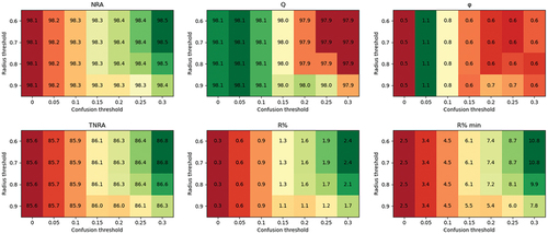
NRA and TNRA (see 2.3.3) increased with the increase in the confusion threshold introduced in the difference probability rejection rule for every site (see 2.3.3) (see Figures 2, 3 and 4). Nevertheless, this increase was notable on all sites for RF and RLR-ℓ1 and in terms of TNRA (increase of 2%, 1.5% and 5% with RF and of 2.5%, 1.5% and 4% with RLR-ℓ1 on sites 1, 2 and 3, respectively). Concerning NRA, RF and RLR-ℓ1 models presented significant changes only on site 3 (of 4% with both models). NRA and TNRA progressions linked to SVMs and RLR-ℓ2 were at a maximum close to 1% and were thus negligible on sites 1 and 2. On the contrary, these three models presented significant variations with the increase in the confusion threshold for site 3. Higher NRA and TNRA values were then observed (increases rising to 2%). Overall, the highest confusion threshold was set, and the greatest was the increases of NRA and TNRA. Moreover, this increase in the confusion threshold allowed an important reduction of the deviations between RF and other algorithms.

Figure 2. Rejection scores associated with simple thresholding on site 1. RF: blue; SVM-linear: red; SVM-RBF: black; RLR-ℓ1: green; RLR-ℓ2: orange. Dashed lines on NRA and Q figures corresponded to OA values without rejection. Dashed lines on the TNRA figure corresponded to TA values without rejection.

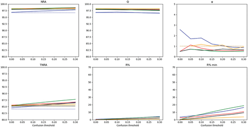
Figure 3. Rejection scores associated with simple thresholding on site 2. RF: blue; SVM-linear: red; SVM-RBF: black; RLR-ℓ1: green; RLR-ℓ2: orange. Dashed lines on NRA and Q figures corresponded to OA values without rejection. Dashed lines on the TNRA figure corresponded to TA values without rejection.

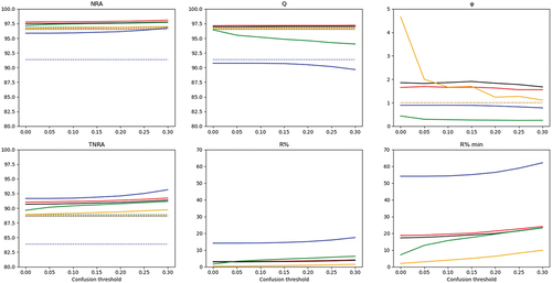
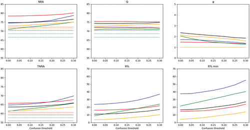
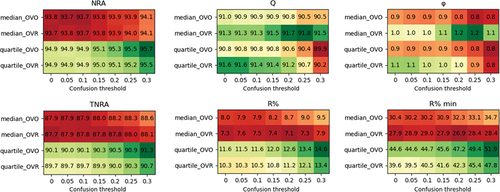
Figure 4. Rejection scores associated with simple thresholding on site 3. RF: blue; SVM-linear: red; SVM-RBF: black; RLR-ℓ1: green; RLR-ℓ2: orange. Dashed lines on NRA and Q figures corresponded to OA values without rejection. Dashed lines on the TNRA figure corresponded to TA values without rejection. The ordinate scale was adapted on NRA, Q and TNRA to the classification performance level related to this site (lower than the two other sites).

The rejection rate among all pixels (${\mathrm{R}}_{\mathrm{\%}}$) and the rejection rate among minor species (${\mathrm{R}}_{\mathrm{\%}\mathrm{m}\mathrm{i}\mathrm{n}}$) increased with the confusion threshold (see Figures 2, 3 and 4). The different behaviours of the evolution of NRA and TNRA with confusion threshold variations were related to different variations in the proportion of rejected pixels. On all sites, the highest increases in rates of rejection were observed with RLR-ℓ1 (between 1.5% and 15% of increase for ${\mathrm{R}}_{\mathrm{\%}}$ and between 16% and 19% for ${\mathrm{R}}_{\mathrm{\%}\mathrm{m}\mathrm{i}\mathrm{n}}$) and RF (4% to 13% and 8% to 18%). Again, smaller variations came with the two SVM models with a low increase in rejection (lower than 6% for $R_{\mathrm{\%}}$and lower than 9% for ${\mathrm{R}}_{\mathrm{\%}\mathrm{m}\mathrm{i}\mathrm{n}}$), and RLR-ℓ2 (lower than 3% for ${\mathrm{R}}_{\mathrm{\%}}$and lower than 6% for ${\mathrm{R}}_{\mathrm{\%}\mathrm{m}\mathrm{i}\mathrm{n}}$). As underlined by these increases, the rejection rate and its increases were highest among minor species for every model and each site. Using the highest confusion threshold would thus lead to rejecting more pixels belonging to all classes but with an emphasis on minor species.

Classification quality criterion Q, which helps to understand differences in NRA, globally did not significantly change according to the chosen confusion threshold. On site 1, Q remained similar to OA whatever the classification model. The same conclusion was provided for site 2, except for RF and RLR-ℓ1 for which Q decreased when increasing the confusion threshold. Thus, the increases observed in NRA, TNRA and rejection rates were achieved at the cost of some rejections among well-classified pixels. Nevertheless, differences between Q and OA stayed low (maximum deviations of 2% and 3% with RF and RLR-ℓ1). On site 3, Q was systematically greater than OA, with differences ranging from 3% to 5%, whatever the chosen confusion threshold.

Finally, rejection quality varied significantly for RLR-ℓ2 on site 2 (−3 when passing from no confusion threshold to 0.3) and RF on site 3 (important variation, decline of 1.5). Other rejection quality criteria did not change significantly with changes in the confusion threshold. According to Condessa et al., if a value of rejection quality is greater than 1, then the rejection was effectively reducing the rate of misclassified pixels (Condessa, Bioucas-Dias, and Kovačević 2017). This condition was verified with some models whatever the confusion threshold for sites 2 and 3. On the contrary, the highest confusion threshold would lead to a rejection quality lower than 1 for all models for site 1, and choosing the highest threshold could thus not be optimal. On this site, this condition was achieved only with a confusion threshold lower than 0.2 with RF and RLR-ℓ2, and 0.1 with SVM-linear. Only the choice of a confusion threshold lower than 0.2 made it possible to maintain a rejection quality greater than 1 for all the sites. This analysis led to choosing a threshold of 0.2 for the reference method to obtain the best NRA, TNRA and ${\mathrm{R}}_{\mathrm{\%}\mathrm{m}\mathrm{i}\mathrm{n}}$ while maintaining a rejection quality greater than 1 for all sites.

Contribution of the rejection class introduction

With a chosen confusion threshold of 0.2, all algorithms performed better or at least equally well with rejection than without. Two exceptions were analysed when regarding the differences between classification quality (Q) and OA on site 2 since a loss of 1% was observed with RF and 2% with RLR-ℓ1. No difference between Q and OA was constated with the other models for this site nor with any of the models on site 1. On the contrary, noticeable progress was observed with all models on site 3 (differences: increase of 2% with RLR-ℓ1 and ℓ2, 3% with SVM-linear, 4% with SVM-RBF and 5% with RF). Overall, adding rejection did not change the classification among predominant species in the simplest scenarios but improved it in the most complex. Similarly, NRA in comparison to OA presented comparable values on site 1. On site 2, a higher NRA than OA came with all models except RLR-ℓ2 (1% increase with RLR- ℓ1 and SVMs, 5% with RF). Scores were increased with all models on site 3 (differences ranging from 3% to 9%).

Finally, the consideration of all species through TA and TNRA highlighted the great improvement brought by rejection since all models presented progress for all sites. Indeed, TNRA was 1% to 2% higher than TA on sites 1 and 2 except with RF with which this improvement amounted to up to 8% on site 2. On site 3, increases were the greatest, ranging from 3% with RLR-ℓ2 and 11% with RF (6% SVM-linear and RLR-ℓ1, 5% SVM-RBF). Thus, rejection particularly improved results for RF, and slightly for RLR-ℓ2. Other models provided intermediate improvement.

Classification model comparison

Even considering rejection, no classification model stood out on all sites. RLR-ℓ2, which provided the best results without rejection, gave the best classification quality on site 1, without exceeding the OA obtained without rejection (Figure 2). However, RLR-ℓ1 provided the best NRA, TNRA and $R_{\mathrm{\%}min}$. Differences with RLR-ℓ2 in terms of NRA, TNRA and classification quality stayed low (inferior to 2%) but differences in terms of rejection of minor species pixels were huge (around 15%). With the chosen threshold of 0.2, RLR-ℓ1 would be the best method to deal with minor species on this specific site. Figure 5 illustrates the resulting map. A few pixels were rejected, and most of them were located at the border between two different classes. The threshold method was thus able to detect some mixed pixels on this site. It should, however, be noted that the rejection quality was lower than 1on this site with this model and, thus, that this minor species and mixed pixels detection led to rejecting pixels a priori well classified. Only RLR-ℓ2 passed this criterion without being related to other significant score variations. Thus, RLR-ℓ2 with rejection would be the most appropriate to deal with predominant classes only.

Figure 5. Classification map of site 1 using RLR-ℓ1 plus rejection using a difference probability rule of 0.2 and corresponding field data (predominant and minor species are delineated in blue and purple, respectively. Rejected pixels are represented in red.

On site 2, SVM-linear provided the best NRA, classification quality and TNRA values. On the other hand, RF led to an equal TNRA value but to the largest number of minor species pixels rejected (Figure 3). RLR-ℓ1, which was the best algorithm without rejection in terms of OA and TA (see Table 3), led to the worst results in terms of rejection quality, and the second lowest in terms of classification quality. Using rejection, the scores values showed that RF was the most appropriate to deal with minor species only and SVM-linear with predominant species. Figure 6 illustrates the differences between the resulting two maps. Both maps showed that mixed pixels, at the edge of different classes, were identified by the rejection methods. However, a lot of pixels were rejected using RF, and numerous pixels should be considered false alarms. These false alarms were highlighted by a rejection quality of 0.9, and thus by a rejection quality slightly lower than 1. If this score allowed the detection of these false alarms, the rejection map analysis was necessary to better judge their importance. In comparison, the rejection map produced owing to the SVM-linear model identified a more suitable number of rejected pixels.

Figure 6. Classification maps of site 2 using RF (left part), SVM-linear (right part) plus rejection with a rejection threshold of 0.2, and in-field data (predominant species are delineated in blue and minor species in purple). Rejected pixels are represented in red.

In the most complex scenario (site 3), results were similar to those obtained for site 2. On those two sites, SVM-RBF with rejection was the best in terms of rejection quality, and the second in terms of classification quality (Figure 4). Nevertheless, since SVM-RBF classification quality was below the one of SVM-linear, SVM-linear with rejection was more appropriate to deal with predominant species (see resulting map Figure 7). Indeed, for this site, SVM-linear provided the best results without rejection (see Table 3), and the best in terms of NRA and classification quality values with rejection. Similar observations could be done on the resulting maps of sites 2 (Figure 6) and 3 (Figure 7). RF led to the detection of most of the pixels corresponding to minor species. Nevertheless, a non-negligible number of pixels from the predominant species were also rejected (false alarms). Unlike the case of site 2, these false alarms were not reflected by a rejection quality lower than 1. A visual assessment of the rejection of minor species and mixed pixels was thus necessary to choose between RF and SVM-linear.

Figure 7. Resulting maps of classification of site 3 using SVM-linear plus rejection using a difference of 0.2, and corresponding field data (predominant species are delineated in blue and minor species in purple). Rejected pixels are represented in red.

3.2.2. K-means

Sensitivity analysis: K-means with rejection needed to optimize a further parameter, the radius threshold. Concerning the confusion rule threshold, the variations and results presented in the previous paragraph remained valid for K-means rejection. On all sites, NRA, TNRA, ${\mathrm{R}}_{\mathrm{\%}}$ and ${\mathrm{R}}_{\mathrm{\%}\mathrm{m}\mathrm{i}\mathrm{n}}$ globally increased with the confusion threshold, while Q remained constant and $\phi$ varied in a non-monotonous way. Variations observed with confusion threshold variations with simple thresholding were found again (see scores associated with SVM-linear on site 1, Figure 8). The choice of a confusion threshold of 0.2 was retained as for the reference method.

Figure 8. Rejection scores of SVM-linear model with K-means rejection on site 1.

More control on rejection was possible through the radius threshold brought by K-means. For the studied configurations (sites, classification models), decreasing the radius threshold (meaning more rejection) led globally to a rise in NRA, TNRA, ${\mathrm{R}}_{\mathrm{\%}}$ and ${\mathrm{R}}_{\mathrm{\%}\mathrm{m}\mathrm{i}\mathrm{n}}$ values (Figure 8). On the contrary, quality scores (Q and $\phi$) and their evolutions according to the radius threshold depended on the model and site.

At the fixed confusion threshold, the classification quality was stable whatever the radius threshold value for sites 1 and 2. In contrast, classification quality increased with an increase in rejection obtained by a reduction in radius threshold on site 3. This increase reached 3.2% (RF). In terms of rejection quality, values were steady for most configurations (variation inferior to 0.3). A more drastic decrease (a loss of 0.6) was noted with RF on site 3.

As done for the confusion threshold fixed to 0.2, the radius threshold was fixed such as choosing the highest rejection while maintaining a rejection quality greater than one for most of the configurations. This led to choosing a radius threshold of 0.7. With this threshold, this criterion was fulfilled by all the models that fulfilled it with simple thresholding plus RF on site 2.

Contribution of the rejection class introduction

Differences with or without K-means rejection provided the same results as those observed with or without simple thresholding on site 1. On the contrary, results were different on sites 2 and 3. First, rejection with RF did not result in a rejection quality lower than 1 with K-means rejection. However, a difference with the reference method was also visible in the corresponding increases in NRA and TNRA values. Indeed, only a 2% progress was observed for NRA (against 5% with the reference method) and 3% for TNRA (against 8%). Finally, increases provided by K-means rejection with all models for site 3 were around 1% lower than those obtained with the reference method.

Classification model comparison

The choice to use K-means rather than thresholding did not lead to any change in the choice of models. While RF associated with K-means rejection provided a rejection quality greater than one on site 2, SVM-linear with K-means provided significantly higher scores (+2% in NRA, +6% in Q, +0.6 in rejection quality and +1% in TNRA). With the fixed thresholds, the following models were retained according to the classification scenario: RLR-ℓ1or RLR-ℓ2 on site 1 depending on whether the emphasis was on the predominant or minor species and SVM-linear on sites 2 and 3.

3.2.3. SVM

Sensitivity analysis

For all the models, using the quartile rule rather than the median one furnished similar NRA and TNRA on site 1 and slightly higher performance on site 3 (+1% to 3% in NRA, +1 to 4% in TNRA). For site 2, only RF led to slightly higher scores (+2% in NRA, +3% in TNRA). These differences were linked to differences in the percentage of rejection (${\mathrm{R}}_{\mathrm{\%}}$, ${\mathrm{R}}_{\mathrm{\%}\mathrm{m}\mathrm{i}\mathrm{n}}$). More rejection was performed using the quartile rule. Differences in rejection rates ranged from 0% to 1% considering all pixels of site 1, from 1% to 5% for site 2 and from 2% to 10% for site 3. Among pixels from minor species, differences were more important on all sites (1% to 4% more pixels rejected with quartile rule in comparison with the median rule for site 1, from 3% to 20% for site 2 and from 3% to 13% for site 3). As observed with other rejection methods, the highest differences were observed with RF, then with RLR-ℓ1, and the lowest with RLR-ℓ2. An illustration of these differences can be seen in Figure 9. To conclude, the quartile rule was retained.

Figure 9. Rejection scores of RF model with SVM rejection on site 2.

Concerning the choice of strategy between OVO and OVR, the results depended on the classification scenario. On site 1, OVR seemed more adapted than OVO since it provided similar NRA and TNRA but higher rejection quality values. For site 2 and the RF model, OVR was better suited (Figure 9). However, for most of the other configurations, OVO appeared better. This strategy was therefore retained.

With this rejection method and retained rules (quartile, OVO), increasing the confusion threshold involved increases in NRA, TNRA and ${\mathrm{R}}_{\mathrm{\%}}$ and ${\mathrm{R}}_{\mathrm{\%}\mathrm{m}\mathrm{i}\mathrm{n}}$ values for all the sites. Q remained stable and the rejection quality trend was overall decreasing with the increase in confusion threshold. To keep rejection quality values greater than one with most algorithms, the choice of a confusion threshold of 0.15 would be more suited but to maintain consistency between rejection methods, the confusion threshold was fixed to 0.2. This choice only affected RF on site 1 (associated rejection quality was reduced from 1 to 0.9). In the other cases, the models providing a rejection quality greater than one were the same as for the reference method.

Contribution of the rejection class introduction

For site 1, the results obtained by the SVM rejection were the same as those obtained by the reference and the K-means methods. For sites 2 and 3 and the RF algorithm, results obtained by the SVM rejection method were comprised between those provided by the reference method and by the K-means rejection (+4% for NRA/OA, −1% for Q/OA and +7% for TNRA/TA for site 2 and +7%, 6% and 8% for site 3). On site 2, the rejection quality associated with RF and SVM rejection was the same as the one obtained by thresholding (0.9) and underlined false alarms of rejections. For other algorithms, differences between K-means and SVM rejection methods were small (<1%).

Classification model comparison

Differences between models were the same as those observed with the other rejection methods. The same models would thus be selected.

3.2.4. Synthesis

Table 4 summarizes the retained parameters for each method. For the three methods, the confusion threshold was fixed at 0.2. RLR-ℓ1 was the most appropriate model to deal with minor species on site 1, but RLR-ℓ2 performed better on predominant species. On both sites 2 and 3, SVM-linear was found to be the greatest model. The choice of a classification model did not change depending on the rejection method.

Table 4. Retained input parameters for each method.

Method	Parameter	Value
Reference method (thresholding)	Confusion threshold	0.2
K-means rejection	Confusion threshold	0.2
	Radius threshold	0.7
SVM rejection	Confusion threshold	0.2
	Strategy	OVO
	Decision function difference threshold	Quartile rule

3.2.5. Rejection method comparison

The three rejection methods with the optimized input parameters (Table 4) and the best models were finally compared using all scores. For site 1, RLR-ℓ1 was selected since the main objective of this study was to deal with the minor species and mixed pixels.

As explained previously, with the chosen thresholds and models, differences between the NRA, TNRA and Q resulting from the different rejection methods were not significant on sites 1 and 2. On site 3, simple thresholding provided the greatest results, followed by SVM-rejection (with differences between 1% and 2% for NRA, and TNRA) and finally K-means rejection (differences of 1% with SVM-rejection for NRA, TNRA and Q).

Nevertheless, the rejection rates (${\mathrm{R}}_{\mathrm{\%}}$ and ${\mathrm{R}}_{\mathrm{\%}\mathrm{m}\mathrm{i}\mathrm{n}}$) changed according to the scenario and rejection method used. For all sites, the most restrictive rejection was provided by simple thresholding. For site 1, K-means was the second most drastic method since it gave a rejection rate (${\mathrm{R}}_{\mathrm{\%}}$) of 2% (versus 3% with the simple thresholding) including 9% among minor species (${\mathrm{R}}_{\mathrm{\%}\mathrm{m}\mathrm{i}\mathrm{n}}$) (versus 13% with the simple thresholding). SVM rejection was the last one: ${\mathrm{R}}_{\mathrm{\%}}$ was equal to 2% and ${\mathrm{R}}_{\mathrm{\%}\mathrm{m}\mathrm{i}\mathrm{n}}$ to 7%. The same ranking resulted for site 2. The simple thresholding method rejected 4% of the referenced pixels (${\mathrm{R}}_{\mathrm{\%}})$ and 21% of pixels belonging to minor species (${\mathrm{R}}_{\mathrm{\%}\mathrm{m}\mathrm{i}\mathrm{n}}$). K-means and SVM rejection methods both rejected 1% fewer pixels overall. K-means rejected 19% of pixels from minor species while SVM rejected only 16%. K-means was thus more precise in its rejections than SVM. On the contrary, for site 3, the difference in the proportion of pixels rejected between all and minor species was in favour of SVM rejection. Indeed, SVM rejected 15% of pixels among minor species and 12% among all species while K-means rejected, respectively, 13% and 12% of pixels and thresholding 19% and 18%. Associated with this, a higher rejection quality was obtained with SVM (higher of 0.4 units) than with the K-means and simple thresholding.

To conclude, the simple thresholding method was the best choice for sites 1 and 2. For site 3, the SVM rejection method was more precise in its rejection even if NRA and TNRA values were slightly lower than those obtained with the simple thresholding method.

4. Discussion

4.1. Supervised classification

4.1.1. Classification scenarios

As mentioned by Fassnacht et al., very few studies in the literature had dealt with multiple sites to evaluate the robustness of machine learning methods (Fabian E. Fassnacht et al. 2014). In this study, three different sites were addressed. Thus, the vegetation mapping of different ecosystems represented by different surface areas (12 ha, 245 ha and 120 ha) was investigated. While the size of an area could already be a challenge for vegetation sampling purposes (Stohlgren et al. 1997), this study considered three different vegetation classification scenarios (vegetation layer classification, species classification of various vegetation types and habitat classification with overlapping classes).

It should be noted that the considered scenarios were all complex. The first site provided a relatively simple classification scenario with a low number of classes. Associated prediction probabilities were high and almost no confusion occurred between classes. While it was an advantage for classification purposes, it made the rejection difficult (see 4.1.2). Other sites presented difficulties related to the high intra-class spectral variability and low inter-class spectral variability which led to confusion among some classes (Zhang et al. 2006).

4.1.2. Supervised classification performance

Performances similar to the one obtained in the state-of-the-art were found in two scenarios. Indeed, the overall accuracies were superior to 90% for the vegetation layer classification and the genera classification as observed for tree species classification based on hyperspectral images (Fabian E. Dian, Zengyuan, and Pang 2015; Fassnacht et al. 2014; Raczko and Zagajewski 2017). On the contrary, a lower performance, close to 70% in OA, was found for site 3, for which classes were overlapping. A similar conclusion was obtained by Burai et al., who improved OA by 70% to 80% after applying dimension reduction techniques (Burai et al. 2015). Such a method could be investigated in the future to improve performance.

A unique optimal algorithm could not be retained to process the three scenarios. This result, in line with previous studies (Fassnacht et al. 2016; Kluczek, Zagajewski, and Zwijacz-Kozica 2023; Lu and Weng 2007), underlined that the choice of the machine learning model depends on the context defined by instrument specifications (e.g. spatial and spectral resolutions), observed scenes, and reference dataset. Several models should be compared for a given vegetation classification application, and the most relevant information related to spectral and spatial instrument characteristics could be analysed as done in recent studies (Erudel et al. 2017; Gimenez et al. 2022; Kluczek, Zagajewski, and Kycko 2022; Kluczek, Zagajewski, and Zwijacz-Kozica 2023).

The consideration of minor species highlighted that the overall accuracy was not sufficient to comprehensively evaluate the resulting vegetation maps. A criterion considering these species, as defined in this study through True Accuracy, could help to improve the quality assessment of the vegetation map. An in-field inventory, with an accurate sampling strategy as proposed for biodiversity evaluation, could be a promising way to evaluate the improvement of such a criterion (Archaux et al. 2006; Gimaret-Carpentier et al. 1998; Keith 2000).

4.2. Rejection

4.2.1. Rejection methods

Previous studies related to vegetation classification highlighted the difficulty of mapping species with a reduced sample number (Kluczek, Zagajewski, and Kycko 2022; Kluczek, Zagajewski, and Zwijacz-Kozica 2023). The rejection methods presented in this study may offer a promising prospect for the management of such species. Indeed, the proposed rejection methods allowed the detection of mixed pixels, a part of the minor species pixels, and an improvement of the scores within the non-rejected pixels. These progress in scores were more pronounced with RF, with which increases rose to 12% considering predominant species only (through NRA) like all species (through TNRA). In line with former works, the importance of rejection was highlighted for the least efficient classification models (Condessa, Bioucas-Dias, and Kovacevic 2015).

If the thresholding method already allowed control of the amount of rejection, K-means and SVM allowed an even greater control thanks to their additional parameters. The control given by the choice of a radius threshold for K-means and by selecting between quartile and median statistics, and OVO and OVR strategy for SVM, allowed more precision during the rejection process for the most difficult scenario (rejection quality increased of 0.4 with SVM compared to the reference method). Nevertheless, the addition of such parameters required more calculation and analysis time for low benefits.

The differences in classification models and chosen thresholds were more important than the rejection method used. Using rejection, the choice of an appropriate model was possible for each scenario. For instance, RLR-ℓ1 was particularly suited for detecting minor species in the vegetation layer classification, while SVM-linear provided the greatest results for other scenarios.

This study focuses on a posteriori rejection methods based on prediction probabilities. While these methods already allowed the detection of some outliers and mixed pixels, it would be appropriate to compare them to other rejection methods. Indeed, the approach proposed here, based on prediction probabilities, has both advantages and drawbacks. Among the advantages, such approaches require only classification results and are reasonably fast since they do not require the processing of large amounts of data such as hyperspectral images. Nevertheless, a notable limitation was observed here on site 1, where low confusion occurred with the classification scenario considered (see 4.1.1). For this specific site, prediction probabilities were high and the approach was thus not appropriate. A rejection method based on spectral behaviour, as defined by Condessa et al., could be a promising way for these specific cases (Condessa et al. 2015). Similarly, the proposed approach could not be appropriate to deal with some machine learning algorithms.

Finally, all resulting maps had shown a salt-and-pepper effect after rejection. Considering the spatial context, as done by Condessa et al., could be a promising and simple way to improve these rejection methods (Condessa et al. 2015).

The approaches were assessed on vegetation classification maps obtained with hyperspectral images at metric spatial resolution. It will be interesting to apply them to classification maps obtained for different spatial resolution ranges. For decametric spatial resolution corresponding to satellite devices, various surface materials lie in the same pixel. For centimetric spatial resolution achieved by a camera embedded in UAV, with the decrease in spatial resolution, the number of mixed pixels increases, and the proposed approaches will be of great interest.

4.2.2. Rejection assessment metrics

Rejection metrics defined in previous studies allowed the evaluation of rejection among predominant classes (Condessa, Bioucas-Dias, and Kovačević 2017). The use of remote sensing data acquired over large scenes ensures the presence of outliers. Metrics dealing with such outliers, as those proposed in this study (True accuracy, True Non-Rejected Accuracy and Rejection rate among minor species) or by Huang, Boom, and Fisher (2015) for fish species classification based on video, should be investigated more deeply on various classification problems. In addition, a lot of mixed pixels seemed to be detected by the rejection methods (visual assessment, see Figure 6 and 7). A quantified evaluation of these rejections would be appropriate. A possible way to assess rejection method quality for mixed pixels could be to perform an automatic mixed pixels localization (Constans et al. 2022), before quantifying the number of mixed pixels rejected.

5. Conclusion

Three different vegetation classification scenarios (vegetation layer classification, genera classification without overlapping classes and vegetation cover classification with overlapping classes), all involving rare species (minor species) and abundant species (predominant species), were considered in this study. For each scenario, the retrieved performance on abundant classes was close to those of the state-of-the-art. Nevertheless, the consideration of minor species through a new score proved that these species could not be ignored for vegetation mapping purposes using remote sensing. Three different a posteriori rejection methods were proposed to deal with these species and mixed pixels. All were able to partly detect corresponding pixels without decreasing classification performance among predominant species. In the future, a posteriori rejection methods and appropriate metrics should be investigated more deeply for various classification contexts (e.g. soil type classification, classification of urban materials, land cover mapping, etc.). With the increasing use of ultra-high-resolution aerial optical cameras and the emergence of new hyperspectral satellites, it will be interesting to assess the rejection methods on a large spatial resolution range covering centimetric to decametric resolution spatial resolution.

Acknowledgements

Airborne data was obtained using the aircraft managed by Safire, the French facility for airborne research, an infrastructure of the French National Centre for Scientific Research (CNRS), Météo-France, and the French National Centre for Space Studies (CNES).

The acquisition of hyperspectral images used in this work was funded by ONERA in the frame of an internal research project named DESSOUS (site 3), by BPI in the frame of the AI4GEO project (site 1), and in the frame of the NAOMI project between TotalEnergies and ONERA (site 2). Part of this research was performed in the framework of the APR SHYMI funded by CNES.

The authors gratefully acknowledge the site managers, the ONERA, CNRS, and TotalEnergies teams for the data preprocessing and their assistance in field sampling, the INSA 4 MA students (J. Gonzales, L. Roig, L. Camusat, E. Etheve) and their professor (D. Sanchez) for their implication in the methodology specifications and software development.

Disclosure statement

No potential conflict of interest was reported by the author(s).

References

- Ahmed, M. M., S. Basu, and A. Kumaravel. 2013. “Clustering Technique for Segmentation of Exudates in Fundus Image.” International Journal of Engineering Sciences & Research Technology 2 (6): 1586–1590.
- Archaux, F., F. Gosselin, L. Bergès, and R. Chevalier. 2006. “Effects of Sampling Time, Species Richness and Observer on the Exhaustiveness of Plant Censuses.” Journal of Vegetation Science 17 (3): 299–306. https://doi.org/10.1111/j.1654-1103.2006.tb02449.x.
- Asner, G. P., R. E. Martin, C. B. Anderson, and D. E. Knapp. 2015. “Quantifying Forest Canopy Traits: Imaging Spectroscopy versus Field Survey.” Remote Sensing of Environment 158: 15–27. Elsevier Inc. https://doi.org/10.1016/j.rse.2014.11.011.
- Aval, J. 2016. “Automatic Mapping of Urban Tree Species Based on Multi-Source Remotely Sensed Data Josselin.” Revue Teledetection 8 (1): 17–34. ( Evolution des propriétés diélectriques, ferroélectriques et électromécaniques dans le système pseudo-binaire (1-x)BaTi0.8Zr0.2O3- xBa0.7Ca0.3TiO3/Corrélations structures et propriétés Feres Benabdallah%0A).
- Breiman, L. 2021. “Random Forest.” Machine Learning 45 (1): 5–32. https://doi.org/10.1109/ICCECE51280.2021.9342376.
- Burai, P., B. Deák, O. Valkó, and T. Tomor. 2015. “Classification of Herbaceous Vegetation Using Airborne Hyperspectral Imagery.” Remote Sensing 7 (2): 2046–2066. https://doi.org/10.3390/rs70202046.
- Cavender-Bares, J., F. D. Schneider, M. João Santos, A. Armstrong, A. Carnaval, K. M. Dahlin, L. Fatoyinbo, et al. 2022. “Integrating Remote Sensing with Ecology and Evolution to Advance Biodiversity Conservation.” Nature Ecology & Evolution Springer US 6 (5): 506–519. https://doi.org/10.1038/s41559-022-01702-5.
- Charoenphakdee, N., Z. Cui, Y. Zhang, and M. Sugiyama. 2020. “Classification with Rejection Based on Cost-Sensitive Classification.” http://arxiv.org/abs/2010.11748.
- Chow, C. 1970. “On Optimum Recognition Error and Reject Tradeoff.” IEEE Transactions on Information Theory 16 (1): 41–46. https://doi.org/10.1109/TIT.1970.1054406.
- Condessa, F., J. Bioucas-Dias, C. A. Castro, J. A. Ozolek, and J. Kovacevic. 2015. “Classification with Reject Option Using Contextual Information.” In Proceedings - International Symposium on Biomedical Imaging, 1340–1343. https://doi.org/10.1109/ISBI.2013.6556780.
- Condessa, F., J. Bioucas-Dias, and J. Kovacevic. 2015. “Supervised Hyperspectral Image Classification with Rejection.” IEEE Journal of Selected Topics in Applied Earth Observations and Remote Sensing 9 (6): 2321–2332. https://doi.org/10.1109/JSTARS.2015.2510032.
- Condessa, F., J. Bioucas-Dias, and J. Kovačević. 2017. “Performance Measures for Classification Systems with Rejection.” Pattern Recognition 63 (February 2016): 437–450. https://doi.org/10.1016/j.patcog.2016.10.011.
- Constans, Y., S. FABRE, H. BRUNET, M. SEYMOUR, V. CROMBEZ, X. BRIOTTET, and J. CHANUSSOT. 2022. “Fusion De Données Hyperspectrales Et Panchromatiques Par Demelange Spectral Dans Le Domaine Reflectif.” Revue Française de Photogrammétrie et de Télédétection 224 (1): 59–74. https://doi.org/10.52638/rfpt.2022.508.
- Cortes, C., G. DeSalvo, and M. Mohri. 2016. “Learning with Rejection.” Lecture Notes in Computer Science (Including Subseries Lecture Notes in Artificial Intelligence & Lecture Notes in Bioinformatics) 9925 LNAI: 67–82. https://doi.org/10.1007/978-3-319-46379-7_5.
- Dian, Y., L. Zengyuan, and Y. Pang. 2015. “Spectral and Texture Features Combined for Forest Tree Species Classification with Airborne Hyperspectral Imagery.” Journal of the Indian Society of Remote Sensing 43 (1): 101–107. https://doi.org/10.1007/s12524-014-0392-6.
- Djeffal, A. 2012. “Utilisation Des Méthodes Support Vector Machine (SVM) Dans l’analyse Des Bases de Données.” Doctoral Dissertation, Université Mohamed Khider-Biskra.
- Erudel, T., S. Fabre, T. Houet, F. Mazier, and X. Briottet. 2017. “Criteria Comparison for Classifying Peatland Vegetation Types Using in situ Hyperspectral Measurements.” Remote Sensing 9 (7). https://doi.org/10.3390/rs9070748.
- Fabre, S., R. Gimenez, A. Elger, and T. Rivière. 2020. “Unsupervised Monitoring Vegetation After the Closure of an Ore Processing Site with Multi-Temporal Optical Remote Sensing.” Sensors (Switzerland) 20 (17): 4800. https://doi.org/10.3390/s20174800.
- Fassnacht, F. E., H. Latifi, K. Stereńczak, A. Modzelewska, M. Lefsky, L. T. Waser, C. Straub, and A. Ghosh. 2016. “Review of Studies on Tree Species Classification from Remotely Sensed Data.” Remote Sensing of Environment 186: 64–87. https://doi.org/10.1016/j.rse.2016.08.013.
- Fassnacht, F. E., C. Neumann, M. Forster, H. Buddenbaum, A. Ghosh, A. Clasen, P. Kumar Joshi, and B. Koch. 2014. “Comparison of Feature Reduction Algorithms for Classifying Tree Species with Hyperspectral Data on Three Central European Test Sites.” IEEE Journal of Selected Topics in Applied Earth Observations and Remote Sensing 7 (6): 2547–2561. https://doi.org/10.1109/JSTARS.2014.2329390.
- Faucon, M. P., D. Houben, and H. Lambers. 2017. “Plant Functional Traits: Soil and Ecosystem Services.” Trends in plant science 22 (5): 385–394. https://doi.org/10.1016/j.tplants.2017.01.005.
- Garcia-Garcia, D., R. Santos-Rodriguez, and E. Parrado-Hernandez. 2012. “Classifier-Based Affinities for Clustering Sets of Vectors.” In 2012 IEEE International Workshop on Machine Learning for Signal Processing, 1–6. IEEE. https://doi.org/10.1109/MLSP.2012.6349760.
- Gimaret-Carpentier, C., R. Pélissier, J.-P. Pascal, and F. Houllier. 1998. “Sampling Strategies for the Assessment of Tree Species Diversity.” Journal of Vegetation Science 9 (2): 161–172. https://doi.org/10.2307/3237115.
- Gimenez, R., G. Lassalle, A. Elger, D. Dubucq, A. Credoz, and S. Fabre. 2022. “Mapping Plant Species in a Former Industrial Site Using Airborne Hyperspectral and Time Series of Sentinel-2 Data Sets.” Remote Sensing 14 (15). https://doi.org/10.3390/rs14153633.
- Givens, C. R., and R. Michael Shortt. 1984. “A Class of Wasserstein Metrics for Probability Distributions.” Michigan Mathematical Journal 31 (2): 231–240. https://doi.org/10.1307/mmj/1029003026.
- Grace, J., E. Mitchard, and E. Gloor. 2014. “Perturbations in the Carbon Budget of the Tropics.” Glob Change Biol 20: 3238–3255. https://doi.org/10.1111/gcb.12600.
- Grandvalet, Y., A. Rakotomamonjy, J. Keshet, and S. Canu. 2011. “Support Vector Machines with a Reject Option.” Bernoulli 17 (4): 1368–1385. https://doi.org/10.3150/10-BEJ320.
- Guichard, L., A. H. Toselli, and C. Bertrand. 2010. Handwritten Word Verification by SVM-Based Hypotheses Re-Scoring and Multiple Thresholds Rejection. IEEE. https://doi.org/10.1109/ICFHR.2010.15.
- Huang, P. X., B. J. Boom, and R. B. Fisher. 2015. “Hierarchical Classification with Reject Option for Live Fish Recognition.” Machine Vision and Applications 26 (1): 89–102. https://doi.org/10.1007/s00138-014-0641-2.
- IPBES. Díaz, S., J. Settele, E. S. Brondízio, H. T. Ngo, M. Guèze, J. Agard, A. Arneth, et al., eds. 2019. Summary for Policymakers of the Global Assessment Report on Biodiversity and Ecosystem Services (Summary for Policy Makers). IPBES Plenary at Its Seventh Session (IPBES 7), Paris. Zenodo. https://doi.org/10.5281/zenodo.3553579.
- Jachowski, N. R. A., M. S. Y. Quak, D. A. Friess, D. Duangnamon, E. L. Webb, and A. D. Ziegler. 2013. “Mangrove Biomass Estimation in Southwest Thailand Using Machine Learning.” Applied Geography 45: 311–321. https://doi.org/10.1016/j.apgeog.2013.09.024.
- Kafle, A., A. Timilsina, A. Gautam, K. Adhikari, A. Bhattarai, and N. Aryal. 2022. “Phytoremediation: Mechanisms, Plant Selection and Enhancement by Natural and Synthetic Agents”. Environmental Advances 8. https://doi.org/10.1016/j.envadv.2022.100203.
- Keith, B. D. A. 2000. “Sampling Designs, Field Techniques and Analytical Methods for Systematic Plant Population Surveys.” Ecological Management & Restoration 1 (2): 125–139. https://doi.org/10.1046/j.1442-8903.2000.00034.x.
- Kluczek, M., B. Zagajewski, and M. Kycko. 2022. “Airborne HySpex Hyperspectral versus Multitemporal Sentinel-2 Images for Mountain Plant Communities Mapping.” Remote Sensing 14 (5). https://doi.org/10.3390/rs14051209.
- Kluczek, M., B. Zagajewski, and T. Zwijacz-Kozica. 2023. “Mountain Tree Species Mapping Using Sentinel-2, PlanetScope, and Airborne HySpex Hyperspectral Imagery.” Remote Sensing 15: 3. https://doi.org/10.3390/rs15030844.
- Laroui, S., X. Descombes, A. Vernay, F. Villiers, F. Villalba, and E. Debreuve. 2021. How to Define a Rejection Class Based on Model Learning? ICPR 2020 - 25th International Conference on Pattern Recognition, Milan / Virtual, Italy. https://doi.org/10.1109/ICPR48806.2021.9412381
- Lu, D., and Q. Weng. 2007. “A Survey of Image Classification Methods and Techniques for Improving Classification Performance.” International Journal of Remote Sensing 28 (5): 823–870. https://doi.org/10.1080/01431160600746456.
- Marcinkowska-Ochtyra, A., B. Zagajewski, A. Ochtyra, A. Jarocińska, B. Wojtuń, C. Rogass, C. Mielke, and S. Lavender. 2017. “Subalpine and Alpine Vegetation Classification Based on Hyperspectral APEX and Simulated EnMap Images.” International Journal of Remote Sensing 38 (7): 1839–1864. Taylor & Francis. https://doi.org/10.1080/01431161.2016.1274447.
- Mori, A. S., K. P. Lertzman, and L. Gustafsson. 2017. “Biodiversity and Ecosystem Services in Forest Ecosystems: A Research Agenda for Applied Forest Ecology.” The Journal of Applied Ecology 54 (1): 12–27. https://doi.org/10.1111/1365-2664.12669.
- Ni, C., C. Nontawat, J. Honda, and S. Masashi. 2019. “On the Calibration of Multiclass Classification with Rejection.” Advances in Neural Information Processing Systems 32 (NeurIPS): 1–11.
- Pant, P., V. Heikkinen, I. Korpela, M. Hauta-Kasari, and T. Tokola. 2014. “Logistic Regression-Based Spectral Band Selection for Tree Species Classification: Effects of Spatial Scale and Balance in Training Samples.” IEEE Geoscience & Remote Sensing Letters 11 (9): 1604–1608. IEEE. https://doi.org/10.1109/LGRS.2014.2301864.
- Paoletti, M. E., J. M. Haut, J. Plaza, and A. Plaza. 2019. “Deep Learning Classifiers for Hyperspectral Imaging: A Review.” Isprs Journal of Photogrammetry & Remote Sensing 158 (November 2018): 279–317. Elsevier. https://doi.org/10.1016/j.isprsjprs.2019.09.006.
- Pedregosa, F., G. Varoquaux, A. Gramfort, V. Michel, B. Thirion, O. Grisel, M. Blondel, et al. 2012. “Scikit-Learn: Machine Learning in Python.” Environmental Health Perspectives 127 (9): 2825–2830. https://doi.org/10.48550/arXiv.1201.0490.
- Petrou, M. 1999. “Mixed Pixel Classification: An Overview.” In Information Processing for Remote Sensing, 69–83. World Scientific.
- Pham, T. D., N. Yokoya, D. Tien Bui, K. Yoshino, and D. A. Friess. 2019. “Remote Sensing Approaches for Monitoring Mangrove Species, Structure, and Biomass: Opportunities and Challenges.” Remote Sensing 11 (3): 1–24. https://doi.org/10.3390/rs11030230.
- Qiu, Z., Z. Feng, Y. Song, L. Menglu, and P. Zhang. 2020. “Carbon Sequestration Potential of Forest Vegetation in China from 2003 to 2050: Predicting Forest Vegetation Growth Based on Climate and the Environment.” Journal of Cleaner Production 252. https://doi.org/10.1016/j.jclepro.2019.119715.
- Raczko, E., and B. Zagajewski. 2017. “Comparison of Support Vector Machine, Random Forest and Neural Network Classifiers for Tree Species Classification on Airborne Hyperspectral APEX Images.” European Journal of Remote Sensing 50 (1): 144–154. Taylor & Francis. https://doi.org/10.1080/22797254.2017.1299557.
- Santos-Pereira, C. M., and A. M. Pires. 2005. “On Optimal Reject Rules and ROC Curves.” Pattern Recognition Letters 26 (7): 943–952. https://doi.org/10.1016/j.patrec.2004.09.042.
- Skidmore, A. K., N. C. Coops, E. Neinavaz, A. Ali, M. E. Schaepman, W. D. K. Marc Paganini, W. D. Kissling, et al. 2021. “Priority List of Biodiversity Metrics to Observe from Space.” Nature Ecology & Evolution 5 (7): 896–906. https://doi.org/10.1038/s41559-021-01451-x.
- Stohlgren, T. J., G. W. Chong, M. A. Kalkhan, and L. D. Schell. 1997. “Multiscale Sampling of Plant Diversity: Effects of Minimum Mapping Unit Size.” Ecological Applications 7 (3): 1064–1074. https://doi.org/10.1890/1051-0761(1997)007[1064:MSOPDE]2.0.CO;2.
- Van, T. V. 2010. Clustering Probability Distributions 4763. https://doi.org/10.1080/02664760903186049.
- Vladimir, V. 1998. The Support Vector Method of Function Estimation. Nonlinear Modeling. https://doi.org/10.7551/mitpress/1130.003.0006.
- Wang, R., and J. A. Gamon. 2019. “Remote Sensing of Terrestrial Plant Biodiversity.” Remote Sensing of Environment 231 (December 2018): 111218. Elsevier. https://doi.org/10.1016/j.rse.2019.111218.
- Wegkamp, M., and M. Yuan. 2011. “Support Vector Machines with a Reject Option.” Bernoulli 17 (4): 1368–1385. https://doi.org/10.3150/10-BEJ320.
- Yuan, M., and M. Wegkamp. 2010. “Classification Methods with Reject Option Based on Convex Risk Minimization.” Journal of Machine Learning Research 11: 111–130.
- Zhang, J., B. Rivard, A. Sánchez-Azofeifa, and K. Castro-Esau. 2006. “Intra- and Inter-Class Spectral Variability of Tropical Tree Species at La Selva, Costa Rica: Implications for Species Identification Using HYDICE Imagery.” Remote Sensing of Environment 105 (2): 129–141. https://doi.org/10.1016/j.rse.2006.06.010.